Post Syndicated from Alex Forster original http://blog.cloudflare.com/building-network-analytics-v2/


Network Analytics v2 is a fundamental redesign of the backend systems that provide real-time visibility into network layer traffic patterns for Magic Transit and Spectrum customers. In this blog post, we'll dive into the technical details behind this redesign and discuss some of the more interesting aspects of the new system.
To protect Cloudflare and our customers against Distributed Denial of Service (DDoS) attacks, we operate a sophisticated in-house DDoS detection and mitigation system called dosd. It takes samples of incoming packets, analyzes them for attacks, and then deploys mitigation rules to our global network which drop any packets matching specific attack fingerprints. For example, a simple network layer mitigation rule might say “drop UDP/53 packets containing responses to DNS ANY queries”.
In order to give our Magic Transit and Spectrum customers insight into the mitigation rules that we apply to their traffic, we introduced a new reporting system called "Network Analytics" back in 2020. Network Analytics is a data pipeline that analyzes raw packet samples from the Cloudflare global network. At a high level, the analysis process involves trying to match each packet sample against the list of mitigation rules that dosd has deployed, so that it can infer whether any particular packet sample was dropped due to a mitigation rule. Aggregated time-series data about these packet samples is then rolled up into one-minute buckets and inserted into a ClickHouse database for long-term storage. The Cloudflare dashboard queries this data using our public GraphQL APIs, and displays the data to customers using interactive visualizations.
What was wrong with v1?
This original implementation of Network Analytics delivered a ton of value to customers and has served us well. However, in the years since it was launched, we have continued to significantly improve our mitigation capabilities by adding entirely new mitigation systems like Advanced TCP Protection (otherwise known as flowtrackd) and Magic Firewall. The original version of Network Analytics only reports on mitigations created by dosd, which meant we had a reporting system that was showing incomplete information.
Adapting the original version of Network Analytics to work with Magic Firewall would have been relatively straightforward. Since firewall rules are “stateless”, we can tell whether a firewall rule matches a packet sample just by looking at the packet itself. That’s the same thing we were already doing to figure out whether packets match dosd mitigation rules.
However, despite our efforts, adapting Network Analytics to work with flowtrackd turned out to be an insurmountable problem. flowtrackd is “stateful”, meaning it determines whether a packet is part of a legitimate connection by tracking information about the other packets it has seen previously. The original Network Analytics design is incompatible with stateful systems like this, since that design made an assumption that the fate of a packet can be determined simply by looking at the bytes inside it.
Rethinking our approach
Rewriting a working system is not usually a good idea, but in this case it was necessary since the fundamental assumptions made by the old design were no longer true. When starting over with Network Analytics v2, it was clear to us that the new design not only needed to fix the deficiencies of the old design, it also had to be flexible enough to grow to support future products that we haven’t even thought of yet. To meet this high bar, we needed to really understand the core principles of network observability.
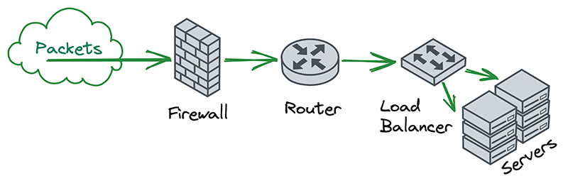
In the world of on-premise networks, packets typically chain through a series of appliances that each serve their own special purposes. For example, a packet may first pass through a firewall, then through a router, and then through a load balancer, before finally reaching the intended destination. The links in this chain can be thought of as independent “network functions”, each with some well-defined inputs and outputs.
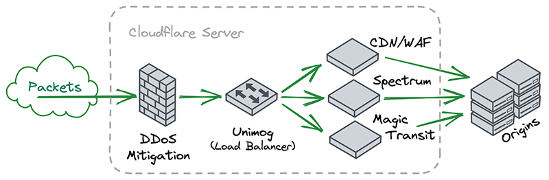
A key insight for us was that, if you squint a little, Cloudflare’s software architecture looks very similar to this. Each server receives packets and chains them through a series of independent and specialized software components that handle things like DDoS mitigation, firewalling, reverse proxying, etc.
After noticing this similarity, we decided to explore how people with traditional networks monitor them. Universally, the answer is either Netflow or sFlow.
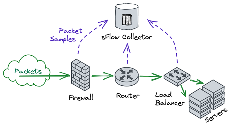
Nearly all on-premise hardware appliances can be configured to send a stream of Netflow or sFlow samples to a centralized flow collector. Traditional network operators tend to take these samples at many different points in the network, in order to monitor each device independently. This was different from our approach, which was to take packet samples only once, as soon as they entered the network and before performing any processing on them.
Another interesting thing we noticed was that Netflow and sFlow samples contain more than just information about packet contents. They also contain lots of metadata, such as the interface that packets entered and exited on, whether they were passed or dropped, which firewall or ACL rule they hit, and more. The metadata format is also extensible, so that devices can include information in their samples which might not make sense for other samples to contain. This flexibility allows flow collectors to offer rich reporting without necessarily having to understand the functions that each device performs on a network.
The more we thought about what kind of features and flexibility we wanted in an analytics system, the more we began to appreciate the elegance of traditional network monitoring. We realized that we could take advantage of the similarities between Cloudflare’s software architecture and “network functions” by having each software component emit its own packet samples with its own context-specific metadata attached.
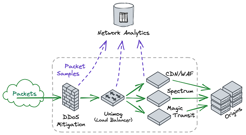
Even though it seemed counterintuitive for our software to emit multiple streams of packet samples this way, we realized through taking inspiration from traditional network monitoring that doing so was exactly how we could build the extensible and future-proof observability that we needed.
Design & implementation
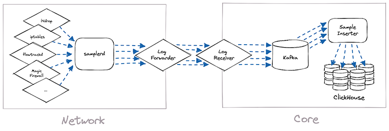
The implementation of Network Analytics v2 could be broken down into two separate pieces of work. First, we needed to build a new data pipeline that could receive packet samples from different sources, then normalize those samples and write them to long-term storage. We called this data pipeline samplerd – the “sampler daemon”.
The samplerd pipeline is relatively small and straightforward. It implements a few different interfaces that other software can use to send it metadata-rich packet samples. It then normalizes these samples and forwards them for postprocessing and insertion into a ClickHouse database.
The other, larger piece of work was to modify existing Cloudflare systems and make them send packet samples to samplerd. The rest of this post will cover a few interesting technical challenges that we had to overcome to adapt these systems to work with samplerd.
l4drop
The first system that incoming packets enter is our xdp daemon, called xdpd. In a few words, xdpd manages the installation of multiple XDP programs: a packet sampler, l4drop and L4LB. l4drop is where many types of attacks are mitigated. Mitigations done at this level are very cheap, because they happen so early in the network stack.
Before introducing samplerd, these XDP programs were organized like this:
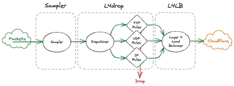
An incoming packet goes through a sampler that will emit a packet sample for some packets. It then enters l4drop, a set of programs that will decide the fate of a particular packet. Finally, L4LB is in charge of layer 4 load balancing.
It’s critical that the samples are emitted even for packets that get dropped further down in the pipeline, because that provides visibility into what’s dropped. That’s useful both from a customer perspective to have a more comprehensive view in dashboards but also to continuously adapt our mitigations as attacks change.
In l4drop’s original configuration, a packet sample is emitted prior to the mitigation decision. Thus, that sample can’t record the mitigation action that’s taken on that particular packet.
samplerd wants packet samples to include the mitigation outcome and other metadata that indicates why a particular mitigation decision was taken. For instance, a packet may be dropped because it matched an attack mitigation signature. Or it may pass because it matched a rate limiting rule and it was under the threshold for that rule. All of this is valuable information that needs to be shown to customers.
Given this requirement, the first idea we had was to simply move the sampler after l4drop and have l4drop just mark the packet as “to be dropped”, along with metadata for the reason why. The sampler component would then have all the necessary details to emit a sample with the final fate of the packet and its associated metadata. After emitting the sample, the sampler would drop or pass the packet.
However, this requires copying all the metadata associated with the dropping decision for every single packet, whether it will be sampled or not. The cost of this copying proved prohibitive considering that every packet entering Cloudflare goes through the xdpd programs.
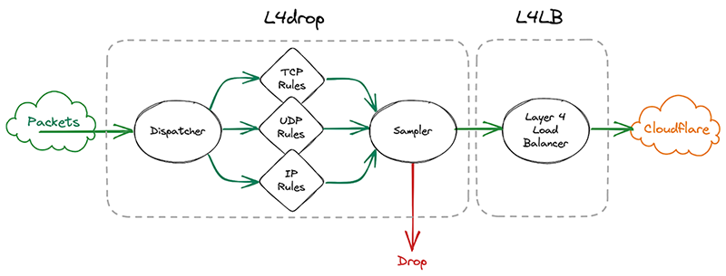
So we went back to the drawing board. What we actually need to know when making a sampling decision is whether we need to copy the metadata. We only need to copy the metadata if a particular packet will be sampled. That’s why it made sense to effectively split the sampler into two parts by sandwiching the programs that make the mitigation decision together. First, we make the mitigation decision, then we go through the mitigation decision programs. These programs can then decide to copy metadata only when a packet will be sampled. They will however always mark a packet with a DROP or PASS mark. Then the sampler will check the mark for sampling and the DROP/PASS mark. Based on those marks, they’ll build a sample if necessary and drop or pass the packet.
Given how tightly the sampler is now coupled with the rest of l4drop, it’s not a standalone part of xdpd anymore and the final result looks like this:
iptables
Another of our mitigation layers is iptables. We use it for some types of mitigations that we can’t perform in l4drop, like stateful connection tracking. iptables mitigations are organized as a list of rules that an incoming packet will be evaluated against. It’s also possible for a rule to jump to another rule when some conditions are met. Some of these rules will perform rate limiting, which will only drop packets beyond a certain threshold. For instance, we might drop all packets beyond a 10 packet-per-second threshold.
Prior to the introduction of samplerd, our typical rules would match on some characteristics of the packet – say, the IP and port – and make a decision whether to immediately drop or pass the packet.
To adapt our iptables rules to samplerd, we need to make them emit annotated samples, so that we can know why a decision was taken. To this end, one idea would be to just make the rules which drop packets also emit a nflog sample with a certain probability. One of the issues with that approach has to do with rate limiting rules. A packet may match such a rule, but the packet may be under the threshold and so that packet gets passed further down the line. That doesn’t work because we also want to sample those passed packets too, since it’s important for a customer to know what was passed and dropped by the rate limiter. But since a packet that passes the rate limiter may be dropped by further rules down the line, it’ll have multiple chances to be sampled, causing oversampling of some parts of the traffic. That would introduce statistical distortions in the sampled data.
To solve this, we can once again separate these steps like we did in l4drop, and make several sets of rules. First, the sampling decision is made by the first set of rules. Then, the pass-or-drop decision is made by the second set of rules. Finally, the sample can be emitted (if necessary), and then the packet can be passed or dropped by the third set of rules.
To communicate between rules we use Linux packet markings. For instance, a mark will be placed on a packet to signal that the packet will be sampled, and another mark will signify that the packet matched a particular rule and that it needs to be dropped.
For incoming packets, the rule in charge of the random sampling decision is evaluated first. Then the mitigation rules are evaluated next, in a specific order. When one of those rules decides to drop a packet, it jumps straight to the last set of rules, which will emit a sample if necessary before dropping. If no mitigation rule matches, eventually packets fall through to the last set of rules, where they will match a generic pass rule. That rule will emit a sample if necessary and pass the packet down the stack for further processing. By organizing rules in stages this way, we won’t ever double-sample packets.
ClickHouse & GraphQL
Once the samplerd daemon has the samples from the various mitigation systems, it does some light processing and ships those samples to be stored in ClickHouse. This inserter further enriches the metadata present in the sample, for instance by identifying the account associated with a particular destination IP. It also identifies ongoing attacks and adds a unique attack ID to each sample that is part of an attack.
We designed the inserters so that we’ll never need to change the data once it has been written, so that we can sustain high levels of insertion. Part of how we achieved this was by using ClickHouse’s MergeTree table engine. However, for improved performance, we have also used a less common ClickHouse table engine, called AggregatingMergeTree. Let’s dive into this using a simplified example.
Each packet sample is stored in a table that looks like the below:
| Attack ID | Dest IP | Dest Port | … | Sample Interval (SI) |
|---|---|---|---|---|
| abcd | 1.1.1.1 | 53 | … | 1000 |
| abcd | 1.0.0.1 | 53 | … | 1000 |
The sample interval is the number of packets that went through between two samples, as we are using ABR.
These tables are then queried through the GraphQL API, either directly or by the dashboard. This required us to build a view of all the samples for a particular attack, to identify (for example) a fixed destination IP. These attacks may span days or even weeks and so these queries could potentially be costly and slow. For instance, a naive query to know whether the attack “abcd” has a fixed destination port or IP may look like this:
SELECT if(uniq(dest_ip) == 1, any(dest_ip), NULL), if(uniq(dest_port) == 1, any(dest_port), NULL)
FROM samples
WHERE attack_id = ‘abcd’
In the above query, we ask ClickHouse for a lot more data than we should need. We only really want to know whether there is one value or multiple values, yet we ask for an estimation of the number of unique values. One way to know if all values are the same (for values that can be ordered) is to check whether the maximum value is equal to the minimum. So we could rewrite the above query as:
SELECT if(min(dest_ip) == max(dest_ip), any(dest_ip), NULL), if(min(dest_port) == max(dest_port), any(dest_port), NULL)
FROM samples
WHERE attack_id = ‘abcd’
And the good news is that storing the minimum or the maximum takes very little space, typically the size of the column itself, as opposed to keeping the state that uniq() might require. It’s also very easy to store and update as we insert. So to speed up that query, we have added a precomputed table with running minimum and maximum using the AggregatingMergeTree engine. This is the special ClickHouse table engine that can compute and store the result of an aggregate function on a particular key. In our case, we will use the attackID as the key to group on, like this:
| Attack ID | min(Dest IP) | max(Dest IP) | min(Dest Port) | max(Dest Port) | … | sum(SI) |
|---|---|---|---|---|---|---|
| abcd | 1.0.0.1 | 1.1.1.1 | 53 | 53 | … | 2000 |
Note: this can be generalized to many aggregating functions like sum(). The constraint on the function is that it gives the same result whether it’s given the whole set all at once or whether we apply the function to the value it returned on a subset and another value from the set.
Then the query that we run can be much quicker and simpler by querying our small aggregating table. In our experience, that table is roughly 0.002% of the original data size, although admittedly all columns of the original table are not present.
And we can use that to build a SQL view that would look like this for our example:
SELECT if(min_dest_ip == max_dest_ip, min_dest_ip, NULL), if(min_dest_port == max_dest_port, min_dest_port, NULL)
FROM aggregated_samples
WHERE attack_id = ‘abcd’
| Attack ID | Dest IP | Dest Port | … | Σ |
|---|---|---|---|---|
| abcd | 53 | … | 2000 |
Implementation detail: in practice, it is possible that a row in the aggregated table gets split on multiple partitions. In that case, we will have two rows for a particular attack ID. So in production we have to take the min or max of all the rows in the aggregating table. That’s usually only three to four rows, so it’s still much faster than going over potentially thousands of samples spanning multiple days. In practice, the query we use in production is thus closer to:
SELECT if(min(min_dest_ip) == max(max_dest_ip), min(min_dest_ip), NULL), if(min(min_dest_port) == max(max_dest_port), min(min_dest_port), NULL)
FROM aggregated_samples
WHERE attack_id = ‘abcd’
Takeaways
Rewriting Network Analytics was a bet that has paid off. Customers now have a more accurate and higher fidelity view of their network traffic. Internally, we can also now troubleshoot and fine tune our mitigation systems much more effectively. And as we develop and deploy new mitigation systems in the future, we are confident that we can adapt our reporting in order to support them.