All posts by Asser Moustafa

Power enterprise-grade Data Vaults with Amazon Redshift – Part 1

Post Syndicated from Asser Moustafa original https://aws.amazon.com/blogs/big-data/power-enterprise-grade-data-vaults-with-amazon-redshift-part-1/

Amazon Redshift is a popular cloud data warehouse, offering a fully managed cloud-based service that seamlessly integrates with an organization’s Amazon Simple Storage Service (Amazon S3) data lake, real-time streams, machine learning (ML) workflows, transactional workflows, and much more—all while providing up to 7.9x better price-performance than other cloud data warehouses.

As with all AWS services, Amazon Redshift is a customer-obsessed service that recognizes there isn’t a one-size-fits-all for customers when it comes to data models, which is why Amazon Redshift supports multiple data models such as Star Schemas, Snowflake Schemas and Data Vault. This post discusses best practices for designing enterprise-grade Data Vaults of varying scale using Amazon Redshift; the second post in this two-part series discusses the most pressing needs when designing an enterprise-grade Data Vault and how those needs are addressed by Amazon Redshift.

Whether it’s a desire to easily retain data lineage directly within the data warehouse, establish a source-system agnostic data model within the data warehouse, or more easily comply with GDPR regulations, customers that implement a Data Vault model will benefit from this post’s discussion of considerations, best practices, and Amazon Redshift features relevant to the building of enterprise-grade Data Vaults. Building a starter version of anything can often be straightforward, but building something with enterprise-grade scale, security, resiliency, and performance typically requires knowledge of and adherence to battle-tested best practices, and using the right tools and features in the right scenario.

Data Vault overview

Let’s first briefly review the core Data Vault premise and concepts. Data models provide a framework for how the data in a data warehouse should be organized into database tables. Amazon Redshift supports a number of data models, and some of the most popular data models include STAR schemas and Data Vault.

Data Vault is not only a modeling methodology, it’s also an opinionated framework that tells you how to solve certain problems in your data ecosystem. An opinionated framework provides a set of guidelines and conventions that developers are expected to follow, rather than leaving all decisions up to the developer. You can compare this with what big enterprise frameworks like Spring or Micronauts do when developing applications at enterprise scale. This is incredibly helpful especially on large data warehouse projects, because it structures your extract, load, and transform (ELT) pipeline and clearly tells you how to solve certain problems within the data and pipeline contexts. This also allows for a high degree of automation.

Data Vault 2.0 allows for the following:

  • Agile data warehouse development
  • Parallel data ingestion
  • A scalable approach to handle multiple data sources even on the same entity
  • A high level of automation
  • Historization
  • Full lineage support

However, Data Vault 2.0 also comes with costs, and there are use cases where it’s not a good fit, such as the following:

  • You only have a few data sources with no related or overlapping data (for example, a bank with a single core system)
  • You have simple reporting with infrequent changes
  • You have limited resources and knowledge of Data Vault

Data Vault typically organizes an organization’s data into a pipeline of four layers: staging, raw, business, and presentation. The staging layer represents data intake and light data transformations and enhancements that occur before the data comes to its more permanent resting place, the raw Data Vault (RDV).

The RDV holds the historized copy of all of the data from multiple source systems. It is referred to as raw because no filters or business transformations have occurred at this point except for storing the data in source system independent targets. The RDV organizes data into three key types of tables:

  • Hubs – This type of table represents a core business entity such as a customer. Each record in a hub table is married with metadata that identifies the record’s creation time, originating source system, and unique business key.
  • Links – This type of table defines a relationship between two or more hubs—for example, how the customer hub and order hub are to be joined.
  • Satellites – This type of table records the historized reference data about either hubs or links, such as product_info and customer_info

The RDV is used to feed data into the business Data Vault (BDV), which is responsible for reorganizing, denormalizing, and aggregating data for optimized consumption by the presentation mart. The presentation marts, also known as the data mart layer, further reorganizes the data for optimized consumption by downstream clients such as business dashboards. The presentation marts may, for example, reorganize data into a STAR schema.

For a more detailed overview of Data Vault along with a discussion of its applicability in the context of very interesting use cases, refer to the following:

How does Data Vault fit into a modern data architecture?

Currently, the lake house paradigm is becoming a major pattern in data warehouse design, even as part of a data mesh architecture. This follows the pattern of data lakes getting closer to what a data warehouse can do and vice versa. To compete with the flexibility of a data lake, Data Vault is a good choice. This way, the data warehouse doesn’t become a bottleneck and you can achieve similar agility, flexibility, scalability, and adaptability when ingestion and onboarding new data.

Platform flexibility

In this section, we discuss some recommended Redshift configurations for Data Vaults of varying scale. As mentioned earlier, the layers within a Data Vault platform are well known. We typically see a flow from the staging layer to the RDV, BDV, and finally presentation mart.

The Amazon Redshift is highly flexible in supporting both modest and large-scale Data Vaults, offering features like the following:

Modest vs. large-scale Data Vaults

Amazon Redshift is flexible in how you decide to structure these layers. For modest data vaults, a single Redshift warehouse with one database with multiple schemas will work just fine.

For large data vaults with more complex transformations, we would look at multiple warehouses, each with their own schema of mastered data representing one or more layer. The reason for using multiple warehouses is to take advantage of the Amazon Redshift architecture’s flexibility for implementing large-scale data vault implementations, such as using Redshift RA3 nodes and Redshift Serverless for separating the compute from the data storage layer and using Redshift data sharing to share the data between different Redshift warehouses. This enables you to scale the compute capacity independently at each layer depending on the processing complexity. The staging layer, for example, can be a layer within your data lake (Amazon S3 storage) or a schema within a Redshift database.

Using Amazon Aurora zero-ETL integrations with Amazon Redshift, you can create a data vault implementation with a staging layer in an Amazon Aurora database that will take care of real-time transaction processing and move the data to Amazon Redshift automatically for further processing in the Data Vault implementation without creating any complex ETL pipelines. This way, you can use Amazon Aurora for transactions and Amazon Redshift for analytics. Compute resources are isolated for the same data, and you’re using the most efficient tools to process it.

Large-scale Data Vaults

For larger Data Vaults platforms, concurrency and compute power become important to process both the loading of data and any business transformations. Amazon Redshift offers flexibility to increase compute capacity both horizontally via concurrency scaling and vertically via cluster resize and also via different architectures for each Data Vault layer.

Staging layer

You can create a data warehouse for the staging layer and perform hard business rules processing here, including calculation of hash keys, hash diffs, and addition of technical metadata columns. If data is not loaded 24/7, consider either pause/resume or a Redshift Serverless workgroup.

Raw Data Vault layer

For raw Data Vault (RDV), it’s recommended to either create one Redshift warehouse for the whole RDV or one Redshift warehouse for one or more subject areas within the RDV. For example, if the volume of data and number of normalized tables within the RDV for a particular subject area is large (either the raw data layer has so many tables that it runs out of maximum table limit on Amazon Redshift or the advantage of workload isolation within a single Redshift warehouse outweighs the overhead of performance and management), this subject area within the RDV can be run and mastered on its own Redshift warehouse.

The RDV is typically loaded 24/7 so a provisioned Redshift data warehouse may be most suitable here to take advantage of reserved instance pricing.

Business Data Vault layer

For creating a data warehouse for the business Data Vault (BDV) layer, this could be larger in size than the previous data warehouses due to the nature of the BDV processing, typically denormalization of data from a large number of source RDV tables.

Some customers run their BDV processing once a day, so a pause/resume window for Redshift provisioned cluster may be cost beneficial here. You can also run BDV processing on an Amazon Redshift Serverless warehouse which will automatically pause when workloads complete and resume when workloads start processing again.

Presentation Data Mart layer

For creating Redshift (provisioned or serverless) warehouses for one or more data marts, the schemas within these marts typically contain views or materialized views, so a Redshift data share will be set up between the data marts and the previous layers.

We need to ensure there is enough concurrency to cope with the increased read traffic at this level. This is achieved via multiple read only warehouses with a data share or the use of concurrency scaling to auto scale.

Example architectures

The following diagram illustrates an example platform for a modest Data Vault model.

The following diagram illustrates the architecture for a large-scale Data Vault model.

Data Vault data model guiding principles

In this section, we discuss some recommended design principles for joining and filtering table access within a Data Vault implementation. These guiding principles address different combinations of entity type access, but should be tested for suitability with each client’s particular use case.

Let’s begin with a brief refresher of table distribution styles in Amazon Redshift. There are four ways that a table’s data can be distributed among the different compute nodes in a Redshift cluster: ALL, KEY, EVEN, and AUTO.

The ALL distribution style ensures that a full copy of the table is maintained on each compute node to eliminate the need for inter-node network communication during workload runs. This distribution style is ideal for tables that are relatively small in size (such as fewer than 5 million rows) and don’t exhibit frequent changes.

The KEY distribution style uses a hash-based approach to persisting a table’s rows in the cluster. A distribution key column is defined to be one of the columns in the row, and the value of that column is hashed to determine on which compute node the row will be persisted. The current generation RA3 node type is built on the AWS Nitro System with managed storage that uses high performance SSDs for your hot data and Amazon S3 for your cold data, providing ease of use, cost-effective storage, and fast query performance. Managed storage means this mapping of row to compute node is more in terms of metadata and compute node ownership rather than the actual persistence. This distribution style is ideal for large tables that have well-known and frequent join patterns on the distribution key column.

The EVEN distribution style uses a round-robin approach to locating a table’s row. Simply put, table rows are cycled through the different compute nodes and when the last compute node in the cluster is reached, the cycle begins again with the next row being persisted to the first compute node in the cluster. This distribution style is ideal for large tables that exhibit frequent table scans.

Finally, the default table distribution style in Amazon Redshift is AUTO, which empowers Amazon Redshift to monitor how a table is used and change the table’s distribution style at any point in the table’s lifecycle for greater performance with workloads. However, you are also empowered to explicitly state a particular distribution style at any point in time if you have a good understanding of how the table will be used by workloads.

Hub and hub satellites

Hub and hub satellites are often joined together, so it’s best to co-locate these datasets based on the primary key of the hub, which will also be part of the compound key of each satellite. As mentioned earlier, for smaller volumes (typically fewer than 5–7 million rows) use the ALL distribution style and for larger volumes, use the KEY distribution style (with the _PK column as the distribution KEY column).

Link and link satellites

Link and link satellites are often joined together, so it’s best to co-locate these datasets based on the primary key of the link, which will also be part of the compound key of each link satellite. These typically involve larger data volumes, so look at a KEY distribution style (with the _PK column as the distribution KEY column).

Point in time and satellites

You may decide to denormalize key satellite attributes by adding them to point in time (PIT) tables with the goal of reducing or eliminating runtime joins. Because denormalization of data helps reduce or eliminate the need for runtime joins, denormalized PIT tables can be defined with an EVEN distribution style to optimize table scans.

However, if you decide not to denormalize, then smaller volumes should use the ALL distribution style and larger volumes should use the KEY distribution style (with the _PK column as the distribution KEY column). Also, be sure to define the business key column as a sort key on the PIT table for optimized filtering.

Bridge and link satellites

Similar to PIT tables, you may decide to denormalize key satellite attributes by adding them to bridge tables with the goal of reducing or eliminating runtime joins. Although denormalization of data helps reduce or eliminate the need for runtime joins, denormalized bridge tables are still typically larger in data volume and involved frequent joins, so the KEY distribution style (with the _PK column as the distribution KEY column) would be the recommended distribution style. Also, be sure to define the bridge of the dominant business key columns as sort keys for optimized filtering.

KPI and reporting

KPI and reporting tables are designed to meet the specific needs of each customer, so flexibility on their structure is key here. These are often standalone tables that exhibit multiple types of interactions, so the EVEN distribution style may be the best table distribution style to evenly spread the scan workloads.

Be sure to choose a sort key that is based on common WHERE clauses such as a date[time] element or a common business key. In addition, a time series table can be created for very large datasets that are always sliced on a time attribute to optimize workloads that typically interact with one slice of time. We discuss this subject in greater detail later in the post.

Non-functional design principles

In this section, we discuss potential additional data dimensions that are often created and married with business data to satisfy non-functional requirements. In the physical data model, these additional data dimensions take the form of technical columns added to each row to enable tracking of non-functional requirements. Many of these technical columns will be populated by the Data Vault framework. The following table lists some of the common technical columns, but you can extend the list as needed.

Column Name Applies to Table Description
LOAD_DTS All A timestamp recording of when this row was inserted. This is a primary key column for historized targets (links, satellites, reference), and a non-primary key column for transactional links and hubs.
BATCH_ID All A unique process ID identifying the run of the ETL code that populated the row.
JOB_NAME All The process name from the ETL framework. This may be a sub-process within a larger process.
SOURCE_SYSTEM_CD All The system from which this data was discovered.
HASH_DIFF Satellite A method in Data Vault of performing change data capture (CDC) changes.
RECORD_ID Satellite
Link
Reference
A unique identifier captured by the code framework for each row.
EFFECTIVE_DTS Link Business effective dates to record the business validity of the row. It’s set to the LOAD_DTS if no business date is present or needed.
DQ_AUDIT Satellite
Link
Reference
Warnings and errors found during staging for this row, tied to the RECORD_ID.

Advanced optimizations and guidelines

In this section, we discuss potential optimizations that can be deployed at the start or later on in the lifecycle of the Data Vault implementation.

Time series tables

Let’s begin with a brief refresher on time series tables as a pattern. Time series tables involve taking a large table and segmenting it into multiple identical tables that hold a time-bound portion of the rows in the original table. One common scenario is to divide a monolithic sales table into monthly or annual versions of the sales table (such as sales_jan,sales_feb, and so on). For example, let’s assume we want to maintain data for a rolling time period using a series of tables, as the following diagram illustrates.

With each new calendar quarter, we create a new table to hold the data for the new quarter and drop the oldest table in the series. Furthermore, if the table rows arrive in a naturally sorted order (such as sales date), then no work is needed to sort the table data, resulting in skipping the expensive VACUUM SORT operation on table.

Time series tables can help significantly optimize workloads that often need to scan these large tables but within a certain time range. Furthermore, by segmenting the data across tables that represent calendar quarters, we are able to drop aged data with a single DROP command. Had we tried to perform the same DELETE operation on a monolithic table design using the DELETE command, for example, it would have been a more expensive deletion operation that would have left the table in a suboptimal state requiring defragmentation and also saves to run a subsequent VACUUM process to reclaim space.

Should a workload ever need to query against the entire time range, you can use standard or materialized views using a UNION ALL operation within Amazon Redshift to easily stitch all the component tables back into the unified dataset. Materialized views can also be used to abstract the table segmentation from downstream users.

In the context of Data Vault, time series tables can be useful for archiving rows within satellites, PIT, and bridge tables that aren’t used often. Time series tables can then be used to distribute the remaining hot rows (rows that are either recently added or referenced often) with more aggressive table properties.

Conclusion

In this post, we discussed a number of areas ripe for optimization and automation to successfully implement a Data Vault 2.0 system at scale and the Amazon Redshift capabilities that you can use to satisfy the related requirements. There are many more Amazon Redshift capabilities and features that will surely come in handy, and we strongly encourage current and prospective customers to reach out to us or other AWS colleagues to delve deeper into Data Vault with Amazon Redshift.


About the Authors

Asser Moustafa is a Principal Analytics Specialist Solutions Architect at AWS based out of Dallas, Texas. He advises customers globally on their Amazon Redshift and data lake architectures, migrations, and visions—at all stages of the data ecosystem lifecycle—starting from the POC stage to actual production deployment and post-production growth.

Philipp Klose is a Global Solutions Architect at AWS based in Munich. He works with enterprise FSI customers and helps them solve business problems by architecting serverless platforms. In this free time, Philipp spends time with his family and enjoys every geek hobby possible.

Saman Irfan is a Specialist Solutions Architect at Amazon Web Services. She focuses on helping customers across various industries build scalable and high-performant analytics solutions. Outside of work, she enjoys spending time with her family, watching TV series, and learning new technologies.

Power enterprise-grade Data Vaults with Amazon Redshift – Part 2

Post Syndicated from Asser Moustafa original https://aws.amazon.com/blogs/big-data/power-enterprise-grade-data-vaults-with-amazon-redshift-part-2/

Amazon Redshift is a popular cloud data warehouse, offering a fully managed cloud-based service that seamlessly integrates with an organization’s Amazon Simple Storage Service (Amazon S3) data lake, real-time streams, machine learning (ML) workflows, transactional workflows, and much more—all while providing up to 7.9x better price-performance than any other cloud data warehouses.

As with all AWS services, Amazon Redshift is a customer-obsessed service that recognizes there isn’t a one-size-fits-all for customers when it comes to data models, which is why Amazon Redshift supports multiple data models such as Star Schemas, Snowflake Schemas and Data Vault. This post discusses the most pressing needs when designing an enterprise-grade Data Vault and how those needs are addressed by Amazon Redshift in particular and AWS cloud in general. The first post in this two-part series discusses best practices for designing enterprise-grade data vaults of varying scale using Amazon Redshift.

Whether it’s a desire to easily retain data lineage directly within the data warehouse, establish a source-system agnostic data model within the data warehouse, or more easily comply with GDPR regulations, customers that implement a data vault model will benefit from this post’s discussion of considerations, best practices, and Amazon Redshift features as well as the AWS cloud capabilities relevant to the building of enterprise-grade data vaults. Building a starter version of anything can often be straightforward, but building something with enterprise-grade scale, security, resiliency, and performance typically requires knowledge and adherence to battle-tested best practices, and using the right tools and features in the right scenario.

Data Vault overview

For a brief review of the core Data Vault premise and concepts, refer to the first post in this series.

In the following sections, we discuss the most common areas of consideration that are critical for Data Vault implementations at scale: data protection, performance and elasticity, analytical functionality, cost and resource management, availability, and scalability. Although these areas can also be critical areas of consideration for any data warehouse data model, in our experience, these areas present their own flavor and special needs to achieve data vault implementations at scale.

Data protection

Security is always priority-one at AWS, and we see the same attention to security every day with our customers. Data security has many layers and facets, ranging from encryption at rest and in transit to fine-grained access controls and more. In this section, we explore the most common data security needs within the raw and business data vaults and the Amazon Redshift features that help achieve those needs.

Data encryption

Amazon Redshift encrypts data in transit by default. With the click of a button, you can configure Amazon Redshift to encrypt data at rest at any point in a data warehouse’s lifecycle, as shown in the following screenshot.

You can use either AWS Key Management Service (AWS KMS) or Hardware Security Module (HSM) to perform encryption of data at rest. If you use AWS KMS, you can either use an AWS managed key or customer managed key. For more information, refer to Amazon Redshift database encryption.

You can also modify cluster encryption after cluster creation, as shown in the following screenshot.

Moreover, Amazon Redshift Serverless is encrypted by default.

Fine-grained access controls

When it comes to achieving fine-grained access controls at scale, Data Vaults typically need to use both static and dynamic access controls. You can use static access controls to restrict access to databases, tables, rows, and columns to explicit users, groups, or roles. With dynamic access controls, you can mask part or all portions of a data item, such as a column based on a user’s role or some other functional analysis of a user’s privileges.

Amazon Redshift has long supported static access controls through the GRANT and REVOKE commands for databases, schemas, and tables, at row level and column level. Amazon Redshift also supports row-level security, where you can further restrict access to particular rows of the visible columns, as well as role-based access control, which helps simplify the management of security privileges in Amazon Redshift.

In the following example, we demonstrate how you can use GRANT and REVOKE statements to implement static access control in Amazon Redshift.

  1. First, create a table and populate it with credit card values:
    -- Create the credit cards table
    
    CREATE TABLE credit_cards 
    ( customer_id INT, 
    is_fraud BOOLEAN, 
    credit_card TEXT);
    
    --populate the table with sample values
    
    INSERT INTO credit_cards 
    VALUES
    (100,'n', '453299ABCDEF4842'),
    (100,'y', '471600ABCDEF5888'),
    (102,'n', '524311ABCDEF2649'),
    (102,'y', '601172ABCDEF4675'),
    (102,'n', '601137ABCDEF9710'),
    (103,'n', '373611ABCDEF6352');
    

  2. Create the user user1 and check permissions for user1 on the credit_cards table. We use SET SESSION AUTHORIZATION to switch to user1 in the current session:
       -- Create user
    
       CREATE USER user1 WITH PASSWORD '1234Test!';
    
       -- Check access permissions for user1 on credit_cards table
       SET SESSION AUTHORIZATION user1; 
       SELECT * FROM credit_cards; -- This will return permission defined error
    

  3. Grant SELECT access on the credit_cards table to user1:
    RESET SESSION AUTHORIZATION;
     
    GRANT SELECT ON credit_cards TO user1;
    

  4. Verify access permissions on the table credit_cards for user1:
    SET SESSION AUTHORIZATION user1;
    
    SELECT * FROM credit_cards; -- Query will return rows
    RESET SESSION AUTHORIZATION;

Data obfuscation

Static access controls are often useful to establish hard boundaries (guardrails) of the user communities that should be able to access certain datasets (for example, only those users that are part of the marketing user group should be allowed access to marketing data). However, what if access controls need to restrict only partial aspects of a field, not the entire field? Amazon Redshift supports partial, full, or custom data masking of a field through dynamic data masking. Dynamic data masking enables you to protect sensitive data in your data warehouse. You can manipulate how Amazon Redshift shows sensitive data to the user at query time without transforming it in the database by using masking policies.

In the following example, we achieve a full redaction of credit card numbers at runtime using a masking policy on the previously used credit_cards table.

  1. Create a masking policy that fully masks the credit card number:
    CREATE MASKING POLICY mask_credit_card_full 
    WITH (credit_card VARCHAR(256)) 
    USING ('000000XXXX0000'::TEXT);

  2. Attach mask_credit_card_full to the credit_cards table as the default policy. Note that all users will see this masking policy unless a higher priority masking policy is attached to them or their role.
    ATTACH MASKING POLICY mask_credit_card_full 
    ON credit_cards(credit_card) TO PUBLIC;

  3. Users will see credit card information being masked when running the following query
    SELECT * FROM credit_cards;

Centralized security policies

You can achieve a great deal of scale by combining static and dynamic access controls to span a broad swath of user communities, datasets, and access scenarios. However, what about datasets that are shared across multiple Redshift warehouses, as might be done between raw data vaults and business data vaults? How can scale be achieved with access controls for a dataset that resides on one Redshift warehouse but is authorized for use across multiple Redshift warehouses using Amazon Redshift data sharing?

The integration of Amazon Redshift with AWS Lake Formation enables centrally managed access and permissions for data sharing. Amazon Redshift data sharing policies are established in Lake Formation and will be honored by all of your Redshift warehouses.

Performance

It is not uncommon for sub-second SLAs to be associated with data vault queries, particularly when interacting with the business vault and the data marts sitting atop the business vault. Amazon Redshift delivers on that needed performance through a number of mechanisms such as caching, automated data model optimization, and automated query rewrites.

The following are common performance requirements for Data Vault implementations at scale:

  • Query and table optimization in support of high-performance query throughput
  • High concurrency
  • High-performance string-based data processing

Amazon Redshift features and capabilities for performance

In this section, we discuss Amazon Redshift features and capabilities that address those performance requirements.

Caching

Amazon Redshift uses multiple layers of caching to deliver subsecond response times for repeat queries. Through Amazon Redshift in-memory result set caching and compilation caching, workloads ranging from dashboarding to visualization to business intelligence (BI) that run repeat queries experience a significant performance boost.

With in-memory result set caching, queries that have a cached result set and no changes to the underlying data return immediately and typically within milliseconds.

The current generation RA3 node type is built on the AWS Nitro System with managed storage that uses high performance SSDs for your hot data and Amazon S3 for your cold data, providing ease of use, cost-effective storage, and fast query performance. In short, managed storage means fast retrieval for your most frequently accessed data and automated/managed identification of hot data by Amazon Redshift.

The large majority of queries in a typical production data warehouse are repeat queries, and data warehouses with data vault implementations observe the same pattern. The most optimal run profile for a repeat query is one that avoids costly query runtime interpretation, which is why queries in Amazon Redshift are compiled during the first run and the compiled code is cached in a global cache, providing repeat queries a significant performance boost.

Materialized views

Pre-computing the result set for repeat queries is a powerful mechanism for boosting performance. The fact that it automatically refreshes to reflect the latest changes in the underlying data is yet another powerful pattern for boosting performance. For example, consider the denormalization queries that might be run on the raw data vault to populate the business vault. It’s quite possible that some less-active source systems will have exhibited little to no changes in the raw data vault since the last run. Avoiding the hit of rerunning the business data vault population queries from scratch in those cases could be a tremendous boost to performance. Redshift materialized views provide that exact functionality by storing the precomputed result set of their backing query.

Queries that are similar to the materialized view’s backing query don’t have to rerun the same logic each time, because they can pull records from the existing result set. Developers and analysts can choose to create materialized views after analyzing their workloads to determine which queries would benefit. Materialized views also support automatic query rewriting to have Amazon Redshift rewrite queries to use materialized views, as well as auto refreshing materialized views, where Amazon Redshift can automatically refresh materialized views with up-to-date data from its base tables.

Alternatively, the automated materialized views (AutoMV) feature provides the same performance benefits of user-created materialized views without the maintenance overhead because Amazon Redshift automatically creates the materialized views based on observed query patterns. Amazon Redshift continually monitors the workload using machine learning and then creates new materialized views when they are beneficial. AutoMV balances the costs of creating and keeping materialized views up to date against expected benefits to query latency. The system also monitors previously created AutoMVs and drops them when they are no longer beneficial. AutoMV behavior and capabilities are the same as user-created materialized views. They are refreshed automatically and incrementally, using the same criteria and restrictions.

Also, whether the materialized views are user-created or auto-generated, Amazon Redshift automatically rewrites queries, without users to change queries, to use materialized views when there is enough of a similarity between the query and the materialized view’s backing query.

Concurrency scaling

Amazon Redshift automatically and elastically scales query processing power to provide consistently fast performance for hundreds of concurrent queries. Concurrency scaling resources are added to your Redshift warehouse transparently in seconds, as concurrency increases, to process read/write queries without wait time. When workload demand subsides, Amazon Redshift automatically shuts down concurrency scaling resources to save you cost. You can continue to use your existing applications and BI tools without any changes.

Because Data Vault allows for highly concurrent data processing and is primarily run within Amazon Redshift, concurrency scaling is the recommended way to handle concurrent transformation operations. You should avoid operations that aren’t supported by concurrency scaling.

Concurrent ingestion

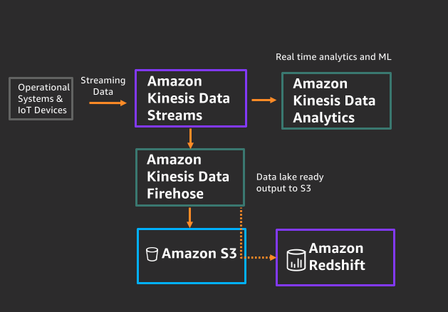
One of the key attractions of Data Vault 2.0 is its ability to support high-volume concurrent ingestion from multiple source systems into the data warehouse. Amazon Redshift provides a number of options for concurrent ingestion, including batch and streaming.

For batch- and microbatch-based ingestion, we suggest using the COPY command in conjunction with CSV format. CSV is well supported by concurrency scaling. In case your data is already on Amazon S3 but in Bigdata formats like ORC or Parquet, always consider the trade-off of converting the data to CSV vs. non-concurrent ingestion. You can also use workload management to prioritize non-concurrent ingestion jobs to keep the throughput high.

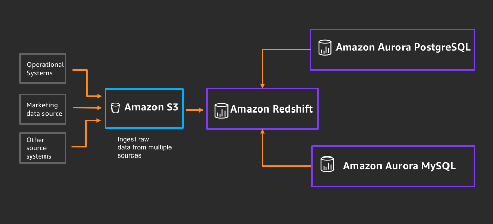
For low-latency workloads, we suggest using the native Amazon Redshift streaming capability or the Amazon Redshift Zero ETL capability in conjunction with Amazon Aurora. By using Aurora as a staging layer for the raw data, you can handle small increments of data efficiently and with high concurrency, and then use this data inside your Redshift data warehouse without any extract, transform, and load (ETL) processes. For stream ingestion, we suggest using the native streaming feature (Amazon Redshift streaming ingestion) and have a dedicated stream for ingesting each table. This might require a stream processing solution upfront, which splits the input stream into the respective elements like the hub and the satellite record.

String-optimized compression

The Data Vault 2.0 methodology often involves time-sensitive lookup queries against potentially very large satellite tables (in terms of row count) that have low-cardinality hash/string indexes. Low-cardinality indexes and very large tables tend to work against time-sensitive queries. Amazon Redshift, however, provides a specialized compression method for low-cardinality string-based indexes called BYTEDICT. Using BYTEDICT creates a dictionary of the low-cardinality string indexes that allow Amazon Redshift to reads the rows even in a compressed state, thereby significantly improving performance. You can manually select the BYTEDICT compression method for a column, or alternatively rely on Amazon Redshift automated table optimization facilities to select it for you.

Support of transactional data lake frameworks

Data Vault 2.0 is an insert-only framework. Therefore, reorganizing data to save money is a challenge you may face. Amazon Redshift integrates seamlessly with S3 data lakes allowing you to perform data lake queries in your S3 using standard SQL as you would with native tables. This way, you can outsource less frequently used satellites to your S3 data lake, which is cheaper than keeping it as a native table.

Modern transactional lake formats like Apache Iceberg are also an excellent option to store this data. They ensure transactional safety and therefore ensure that your audit trail, which is a fundamental feature of Data Vault, doesn’t break.

We also see customers using these frameworks as a mechanism to implement incremental loads. Apache Iceberg lets you query for the last state for a given point in time. You can use this mechanism to optimize merge operations while still making the data accessible from within Amazon Redshift.

Amazon Redshift data sharing performance considerations

For large-scale Data Vault implementation, one of the preferred design principals is to have a separate Redshift data warehouse for each layer (staging, raw Data Vault, business Data Vault, and presentation data mart). These layers have separate Redshift provisioned or serverless warehouses according to their storage and compute requirements and use Amazon Redshift data sharing to share the data between these layers without physically moving the data.

Amazon Redshift data sharing enables you to seamlessly share live data across multiple Redshift warehouses without any data movement. Because the data sharing feature serves as the backbone in implementing large-scale Data Vaults, it’s important to understand the performance of Amazon Redshift in this scenario.

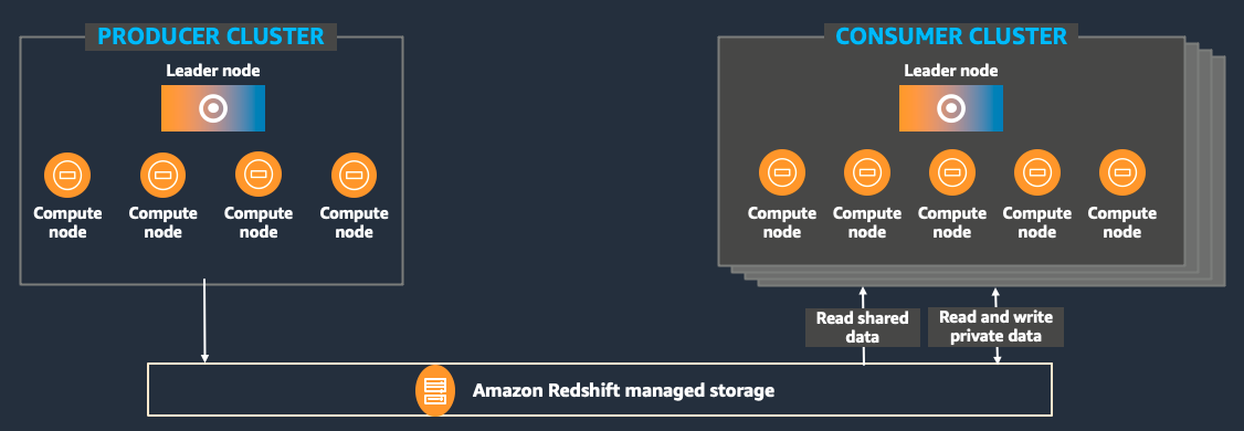
In a data sharing architecture, we have producer and consumer Redshift warehouses. The producer warehouse shares the data objects to one or more consumer warehouse for read purposes only without having to copy the data.

Producer/consumer Redshift cluster performance dependency

From a performance perspective, the producer (provisioned or serverless) warehouse is not responsible for query performance running on the consumer (provisioned or serverless) warehouse and has zero impact in terms of performance or activity on the producer Redshift warehouse. It depends on the consumer Redshift warehouse compute capacity. The producer warehouse is only responsible for the shared data.

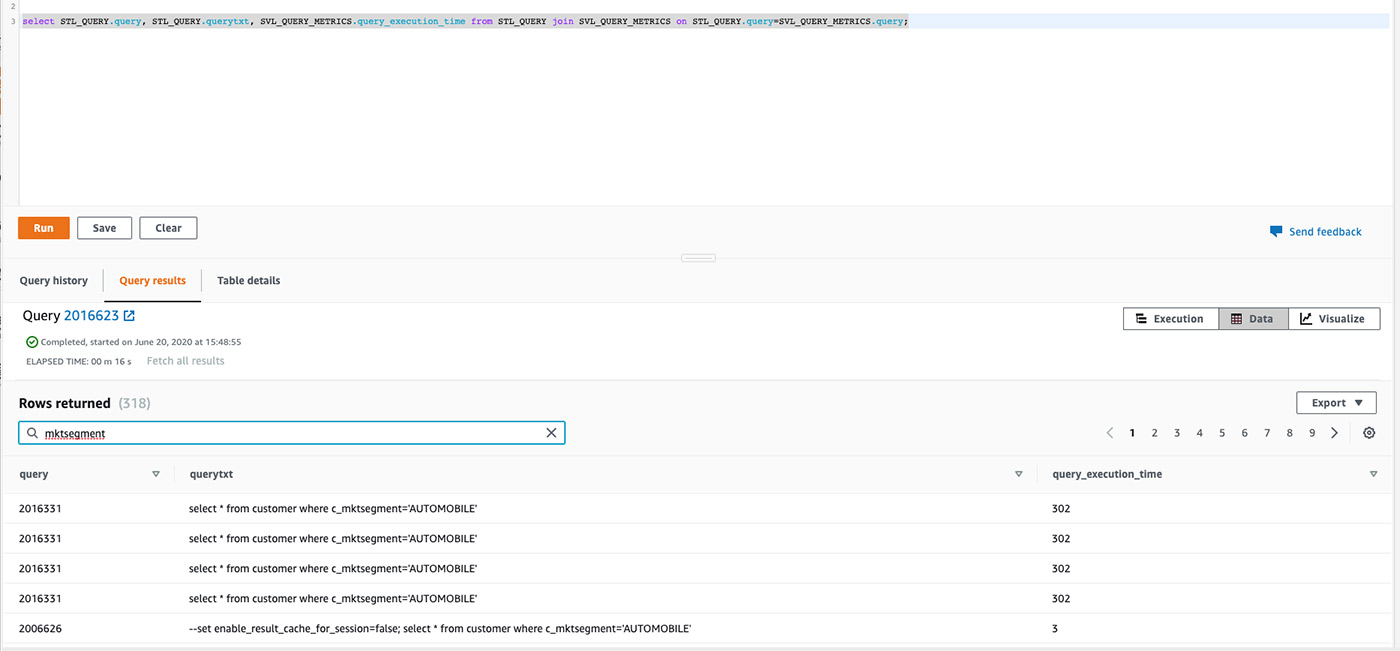
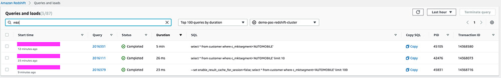
Result set caching on the consumer Redshift cluster

Amazon Redshift uses result set caching to speed up the retrieval of data when it knows that the data in the underlying table has not changed. In a data sharing architecture, Amazon Redshift also uses result set caching on the consumer Redshift warehouse. This is quite helpful for repeatable queries that commonly occur in a data warehousing environment.

Best practices for materialized views in Data Vault with Amazon Redshift data sharing

In Data Vault implementation, the presentation data mart layer typically contains views or materialized views. There are two possible routes to create materialized views for the presentation data mart layer. First, create the materialized views on the producer Redshift warehouse (business data vault layer) and share materialized views with the consumer Redshift warehouse (dedicated data marts). Alternatively, share the table objects directly from the business data vault layer to the presentation data mart layer and build the materialized view on the shared objects directly on the consumer Redshift warehouse.

The second option is recommended in this case, because it gives us the flexibility of creating customized materialized views of data on each consumer according to the specific use case and simplifies the management because each data mart user can create and manage materialized views on their own Redshift warehouse rather than be dependent on the producer warehouse.

Table distribution implications in Amazon Redshift data sharing

Table distribution style and how data is distributed across Amazon Redshift plays a significant role in query performance. In Amazon Redshift data sharing, the data is distributed on the producer Redshift warehouse according to the distribution style defined for table. When we associate the data via a data share to the consumer Redshift warehouse, it maps to the same disk block layout. Also, a bigger consumer Redshift warehouse will result in better query performance for queries running on it.

Concurrency scaling

Concurrency scaling is also supported on both producer and consumer Redshift warehouses for read and write operations.

Cost and resource management

Given that multiple source systems and users will interact heavily with the data vault data warehouse, it’s a prudent best practice to enable usage and query limits to serve as guardrails against runaway queries and unapproved usage patterns. Furthermore, it often helps to have a systematic way for allocating service costs based on usage of the data vault to different source systems and user groups within your organization.

The following are common cost and resource management requirements for Data Vault implementations at scale:

  • Utilization limits and query resource guardrails
  • Advanced workload management
  • Chargeback capabilities

Amazon Redshift features and capabilities for cost and resource management

In this section, we discuss Amazon Redshift features and capabilities that address those cost and resource management requirements.

Utilization limits and query monitoring rules

Runaway queries and excessive auto scaling are likely to be the two most common runaway patterns observed with data vault implementations at scale.

A Redshift provisioned cluster supports usage limits for features such as Redshift Spectrum, concurrency scaling, and cross-Region data sharing. A concurrency scaling limit specifies the threshold of the total amount of time used by concurrency scaling in 1-minute increments. A limit can be specified for a daily, weekly, or monthly period (using UTC to determine the start and end of the period).

You can also define multiple usage limits for each feature. Each limit can have a different action, such as logging to system tables, alerting via Amazon CloudWatch alarms and optionally Amazon Simple Notification Service (Amazon SNS) subscriptions to that alarm (such as email or text), or disabling the feature outright until the next time period begins (such as the start of the month). When a usage limit threshold is reached, events are also logged to a system table.

Redshift provisioned clusters also support query monitoring rules to define metrics-based performance boundaries for workload management queues and the action that should be taken when a query goes beyond those boundaries. For example, for a queue dedicated to short-running queries, you might create a rule that cancels queries that run for more than 60 seconds. To track poorly designed queries, you might have another rule that logs queries that contain nested loops.

Each query monitoring rule includes up to three conditions, or predicates, and one query action (such as stop, hop, or log). A predicate consists of a metric, a comparison condition (=, <, or >), and a value. If all of the predicates for any rule are met, that rule’s action is triggered. Amazon Redshift evaluates metrics every 10 seconds and if more than one rule is triggered during the same period, Amazon Redshift initiates the most severe action (stop, then hop, then log).

Redshift Serverless also supports usage limits where you can specify the base capacity according to your price-performance requirements. You can also set the maximum RPU (Redshift Processing Units) hours used per day, per week, or per month to keep the cost predictable and specify different actions, such as write to system table, receive an alert, or turn off user queries when the limit is reached. A cross-Region data sharing usage limit is also supported, which limits how much data transferred from the producer Region to the consumer Region that consumers can query.

You can also specify query limits in Redshift Serverless to stop poorly performing queries that exceed the threshold value.

Auto workload management

Not all queries have the same performance profile or priority, and data vault queries are no different. Amazon Redshift workload management (WLM) adapts in real time to the priority, resource allocation, and concurrency settings required to optimally run different data vault queries. These queries could consist of a high number of joins between the hubs, links, and satellites tables; large-scale scans of the satellite tables; or massive aggregations. Amazon Redshift WLM enables you to flexibly manage priorities within workloads so that, for example, short or fast-running queries won’t get stuck in queues behind long-running queries.

You can use automatic WLM to maximize system throughput and use resources effectively. You can enable Amazon Redshift to manage how resources are divided to run concurrent queries with automatic WLM. Automatic WLM manages the resources required to run queries. Amazon Redshift determines how many queries run concurrently and how much memory is allocated to each dispatched query.

Chargeback metadata

Amazon Redshift provides different pricing models to cater to different customer needs. On-demand pricing offers the greatest flexibility, whereas Reserved Instances provide significant discounts for predictable and steady usage scenarios. Redshift Serverless provides a pay-as-you-go model that is ideal for sporadic workloads.

However, with any of these pricing models, Amazon Redshift customers can attribute cost to different users. To start, Amazon Redshift provides itemized billing like many other AWS services in AWS Cost Explorer to attain the overall cost of using Amazon Redshift. Moreover, the cross-group collaboration (data sharing) capability of Amazon Redshift enables a more explicit and structured chargeback model to different teams.

Availability

In the modern data organization, data warehouses are no longer used purely to perform historical analysis in batches overnight with relatively forgiving SLAs, Recovery Time Objectives (RTOs), and Recovery Point Objectives (RPOs). They have become mission-critical systems in their own right that are used for both historical analysis and near-real-time data analysis. Data Vault systems at scale very much fit that mission-critical profile, which makes availability key.

The following are common availability requirements for Data Vault implementations at scale:

  • RTO of near-zero
  • RPO of near-zero
  • Automated failover
  • Advanced backup management
  • Commercial-grade SLA

Amazon Redshift features and capabilities for availability

In this section, we discuss the features and capabilities in Amazon Redshift that address those availability requirements.

Separation of storage and compute

AWS and Amazon Redshift are inherently resilient. With Amazon Redshift, there’s no additional cost for active-passive disaster recovery. Amazon Redshift replicates all of your data within your data warehouse when it is loaded and also continuously backs up your data to Amazon S3. Amazon Redshift always attempts to maintain at least three copies of your data (the original and replica on the compute nodes, and a backup in Amazon S3).

With separation of storage and compute and Amazon S3 as the persistence layer, you can achieve an RPO of near-zero, if not zero itself.

Cluster relocation to another Availability Zone

Amazon Redshift provisioned RA3 clusters support cluster relocation to another Availability Zone in events where cluster operation in the current Availability Zone is not optimal, without any data loss or changes to your application. Cluster relocation is available free of charge; however, relocation might not always be possible if there is a resource constraint in the target Availability Zone.

Multi-AZ deployment

For many customers, the cluster relocation feature is sufficient; however, enterprise data warehouse customers require a low RTO and higher availability to support their business continuity with minimal impact to applications.

Amazon Redshift supports Multi-AZ deployment for provisioned RA3 clusters.

A Redshift Multi-AZ deployment uses compute resources in multiple Availability Zones to scale data warehouse workload processing as well as provide an active-active failover posture. In situations where there is a high level of concurrency, Amazon Redshift will automatically use the resources in both Availability Zones to scale the workload for both read and write requests using active-active processing. In cases where there is a disruption to an entire Availability Zone, Amazon Redshift will continue to process user requests using the compute resources in the sister Availability Zone.

With features such as multi-AZ deployment, you can achieve a low RTO, should there ever be a disruption to the primary Redshift cluster or an entire Availability Zone.

Automated backup

Amazon Redshift automatically takes incremental snapshots that track changes to the data warehouse since the previous automated snapshot. Automated snapshots retain all of the data required to restore a data warehouse from a snapshot. You can create a snapshot schedule to control when automated snapshots are taken, or you can take a manual snapshot any time.

Automated snapshots can be taken as often as once every hour and retained for up to 35 days at no additional charge to the customer. Manual snapshots can be kept indefinitely at standard Amazon S3 rates. Furthermore, automated snapshots can be automatically replicated to another Region and stored there as a disaster recovery site also at no additional charge (with the exception of data transfer charges across Regions) and manual snapshots can also be replicated with standard Amazon S3 rates applying (and data transfer costs).

Amazon Redshift SLA

As a managed service, Amazon Redshift frees you from being the first and only line of defense against disruptions. AWS will use commercially reasonable efforts to make Amazon Redshift available with a monthly uptime percentage for each Multi-AZ Redshift cluster during any monthly billing cycle, of at least 99.99% and for multi-node cluster, at least 99.9%. In the event that Amazon Redshift doesn’t meet the Service Commitment, you will be eligible to receive a Service Credit.

Scalability

One of the major motivations of organizations migrating to the cloud is improved and increased scalability. With Amazon Redshift, Data Vault systems will always have a number of scaling options available to them.

The following are common scalability requirements for Data Vault implementations at scale:

  • Automated and fast-initiating horizontal scaling
  • Robust and performant vertical scaling
  • Data reuse and sharing mechanisms

Amazon Redshift features and capabilities for scalability

In this section, we discuss the features and capabilities in Amazon Redshift that address those scalability requirements.

Horizontal and vertical scaling

Amazon Redshift uses concurrency scaling automatically to support virtually unlimited horizontal scaling of concurrent users and concurrent queries, with consistently fast query performance. Furthermore, concurrency scaling requires no downtime, supports read/write operations, and is typically the most impactful and used scaling option for customers during normal business operations to maintain consistent performance.

With Amazon Redshift provisioned warehouse, as your data warehousing capacity and performance needs to change or grow, you can vertically scale your cluster to make the best use of the computing and storage options that Amazon Redshift provides. Resizing your cluster by changing the node type or number of nodes can typically be achieved in 10–15 minutes. Vertical scaling typically occurs much less frequently in response to persistent and organic growth and is typically performed during a planned maintenance window when the short downtime doesn’t impact business operations.

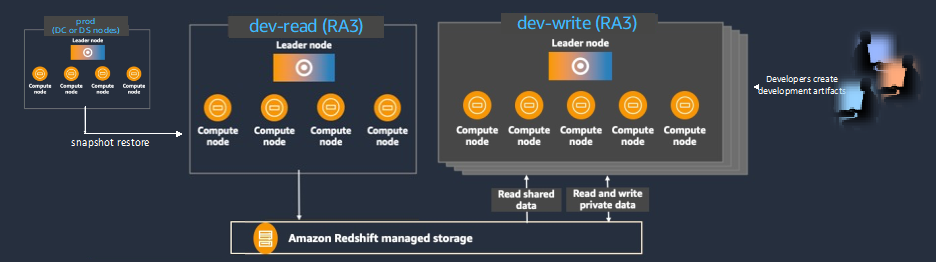
Explicit horizontal or vertical resize and pause operations can be automated per a schedule (for example, development clusters can be automatically scaled down or paused for the weekends). Note that the storage of paused clusters remains accessible to clusters with which their data was shared.

For resource-intensive workloads that might benefit from a vertical scaling operation vs. concurrency scaling, there are also other best-practice options that avoid downtime, such as deploying the workload onto its own Redshift Serverless warehouse while using data sharing.

Redshift Serverless measures data warehouse capacity in RPUs, which are resources used to handle workloads. You can specify the base data warehouse capacity Amazon Redshift uses to serve queries (ranging from as little as 8 RPUs to as high as 512 RPUs) and change the base capacity at any time.

Data sharing

Amazon Redshift data sharing is a secure and straightforward way to share live data for read purposes across Redshift warehouses within the same or different accounts and Regions. This enables high-performance data access while preserving workload isolation. You can have separate Redshift warehouses, either provisioned or serverless, for different use cases according to your compute requirement and seamlessly share data between them.

Common use cases for data sharing include setting up a central ETL warehouse to share data with many BI warehouses to provide read workload isolation and chargeback, offering data as a service and sharing data with external consumers, multiple business groups within an organization, sharing and collaborating on data to gain differentiated insights, and sharing data between development, test, and production environments.

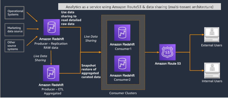
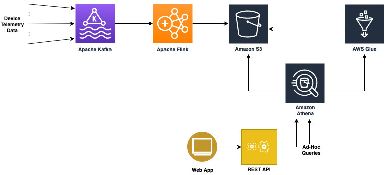
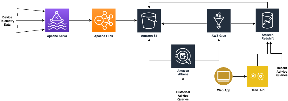
Reference architecture

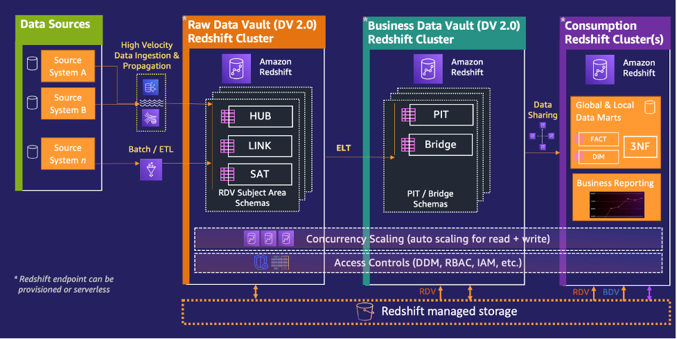
The diagram in this section shows one possible reference architecture of a Data Vault 2.0 system implemented with Amazon Redshift.

We suggest using three different Redshift warehouses to run a Data Vault 2.0 model in Amazon Redshift. The data between these data warehouses is shared via Amazon Redshifts data sharing and allows you to consume data from a consumer data warehouse even if the provider data warehouse is inactive.

  • Raw Data Vault – The RDV data warehouse hosts hubs, links, and satellite tables. For large models, you can additionally slice the RDV into additional data warehouses to even better adopt the data warehouse sizing to your workload patterns. Data is ingested via the patterns described in the previous section as batch or high velocity data.
  • Business Data Vault – The BDV data warehouse hosts bridge and point in time (PIT) tables. These tables are computed based on the RDV tables using Amazon Redshift. Materialized or automatic materialized views are straightforward mechanisms to create those.
  • Consumption cluster – This data warehouse contains query-optimized data formats and marts. Users interact with this layer.

If the workload pattern is unknown, we suggest starting with a Redshift Serverless warehouse and learning the workload pattern. You can easily migrate between a serverless and provisioned Redshift cluster at a later stage based on your processing requirements, as discussed in Part 1 of this series.

Best practices building a Data Vault warehouse on AWS

In this section, we cover how the AWS Cloud as a whole plays its role in building an enterprise-grade Data Vault warehouse on Amazon Redshift.

Education

Education is a fundamental success factor. Data Vault is more complex than traditional data modeling methodologies. Before you start the project, make sure everyone understands the principles of Data Vault. Amazon Redshift is designed to be very easy to use, but to ensure the most optimal Data Vault implementation on Amazon Redshift, gaining a good understanding of how Amazon Redshift works is recommended. Start with free resources like reaching out to your AWS account representative to schedule a free Amazon Redshift Immersion Day or train for the AWS Analytics specialty certification.

Automation

Automation is a major benefit of Data Vault. This will increase efficiency and consistency across your data landscape. Most customers focus on the following aspects when automating Data Vault:

  • Automated DDL and DML creation, including modeling tools especially for the raw data vault
  • Automated ingestion pipeline creation
  • Automated metadata and lineage support

Depending on your needs and skills, we typically see three different approaches:

  • DSL – This is a common tool for generating data vault models and flows with Domain Specific Languages (DSL). Popular frameworks for building such DSLs are EMF with Xtext or MPS. This solution provides the most flexibility. You directly build your business vocabulary into the application and generate documentation and business glossary along with the code. This approach requires the most skill and biggest resource investment.
  • Modeling tool – You can build on an existing modeling language like UML 2.0. Many modeling tools come with code generators. Therefore, you don’t need to build your own tool, but these tools are often hard to integrate into modern DevOps pipelines. They also require UML 2.0 knowledge, which raises the bar for non-tech users.
  • Buy – There are a number of different third-party solutions that integrate well into Amazon Redshift and are available via AWS Marketplace.

Whichever approach of the above-mentioned approaches you choose, all three approaches offer multiple benefits. For example, you can take away repetitive tasks from your development team and enforce modeling standards like data types, data quality rules, and naming conventions. To generate the code and deploy it, you can use AWS DevOps services. As part of this process, you save the generated metadata to the AWS Glue Data Catalog, which serves as a central technical metadata catalog. You then deploy the generated code to Amazon Redshift (SQL scripts) and to AWS Glue.

We designed AWS CloudFormation for automation; it’s the AWS-native way of automating infrastructure creation and management. A major use case for infrastructure as code (IaC) is to create new ingestion pipelines for new data sources or add new entities to existing one.

You can also use our new AI coding tool Amazon CodeWhisperer, which helps you quickly write secure code by generating whole line and full function code suggestions in your IDE in real time, based on your natural language comments and surrounding code. For example, CodeWhisperer can automatically take a prompt such as “get new files uploaded in the last 24 hours from the S3 bucket” and suggest appropriate code and unit tests. This can greatly reduce development effort in writing code, for example for ETL pipelines or generating SQL queries, and allow more time for implementing new ideas and writing differentiated code.

Operations

As previously mentioned, one of the benefits of Data Vault is the high level of automation which, in conjunction with serverless technologies, can lower the operating efforts. On the other hand, some industry products come with built-in schedulers or orchestration tools, which might increase operational complexity. By using AWS-native services, you’ll benefit from integrated monitoring options of all AWS services.

Conclusion

In this series, we discussed a number of crucial areas required for implementing a Data Vault 2.0 system at scale, and the Amazon Redshift capabilities and AWS ecosystem that you can use to satisfy those requirements. There are many more Amazon Redshift capabilities and features that will surely come in handy, and we strongly encourage current and prospective customers to reach out to us or other AWS colleagues to delve deeper into Data Vault with Amazon Redshift.


About the Authors

Asser Moustafa is a Principal Analytics Specialist Solutions Architect at AWS based out of Dallas, Texas. He advises customers globally on their Amazon Redshift and data lake architectures, migrations, and visions—at all stages of the data ecosystem lifecycle—starting from the POC stage to actual production deployment and post-production growth.

Philipp Klose is a Global Solutions Architect at AWS based in Munich. He works with enterprise FSI customers and helps them solve business problems by architecting serverless platforms. In this free time, Philipp spends time with his family and enjoys every geek hobby possible.

Saman Irfan is a Specialist Solutions Architect at Amazon Web Services. She focuses on helping customers across various industries build scalable and high-performant analytics solutions. Outside of work, she enjoys spending time with her family, watching TV series, and learning new technologies.

Power highly resilient use cases with Amazon Redshift

Post Syndicated from Asser Moustafa original https://aws.amazon.com/blogs/big-data/power-highly-resilient-use-cases-with-amazon-redshift/

Amazon Redshift is the most popular and fastest cloud data warehouse, offering seamless integration with your data lake and other data sources, up to three times faster performance than any other cloud data warehouse, automated maintenance, separation of storage and compute, and up to 75% lower cost than any other cloud data warehouse. This post explores different architectures and use cases that focus on maximizing data availability, using Amazon Redshift as the core data warehouse platform.

In the modern data-driven organization, many data analytics use cases using Amazon Redshift have increasingly evolved to assume a critical business profile. Those use cases are now required to be highly resilient with little to no downtime. For example, analytical use cases that once relied solely on historical data and produced static forecasts are now expected to continuously weave real-time streaming and operational data into their ever-updating analytical forecasts. Machine learning (ML) use cases that relied on overnight batch jobs to extract customer churn predictions from extremely large datasets are now expected to perform those same customer churn predictions on demand using both historical and intraday datasets.

This post is part one of a series discussing high resiliency and availability with Amazon Redshift. In this post, we discuss a diverse set of popular analytical use cases that have traditionally or perhaps more recently assumed a critical business profile. The goal of this post is to show the art of the possible with high resiliency use cases. For each use case, we provide a brief description and explore the reasons for its critical business profile, and provide a reference architecture for implementing the use case following best practices. In the following section, we include a brief mention of some of the complimentary high resiliency features in Amazon Redshift as they apply for each use case.

In the final section of this post, we expand the scope to discuss high resiliency in a data ecosystem that uses Amazon Redshift. In particular, we discuss the Lake House Architecture in the high resiliency context.

Part two of this series (coming soon) provides a deeper look into the individual high resiliency and availability features of Amazon Redshift.

Now let’s explore some of the most popular use cases that have traditionally required high resiliency or have come to require high resiliency in the modern data-driven organization.

Data analytics as a service

Many analytical use cases focus on extracting value from data collected and produced by an organization to serve the organization’s internal business and operational goals. In many cases, however, the data collected and produced by an organization can itself be packaged and offered as a product to other organizations. More specifically, access to the data collected and produced along with analytical capabilities is typically offered as a paid service to other organizations. This is referred to as data analytics as a service (DaaS).

For example, consider a marketing agency that has amassed demographic information for a geographic location such as population by age, income, and family structure. Such demographic information often serves as a vital input for many organizations’ decisions to identify the ideal location for expansion, match their products with likely buyers, product offerings, and many other business needs. The marketing agency can offer access to this demographic information as a paid service to a multitude of retailers, healthcare providers, resorts, and more.

Some of the most critical aspects of DaaS offerings are ease of management, security, cost-efficiency, workload isolation, and high resiliency and availability. For example, the marketing agency offering the DaaS product needs the ability to easily refresh the demographic data on a regular cadence (ease of management), ensure paying customers are able to access only authorized data (security), minimize data duplication to avoid runaway costs and keep the DaaS competitively priced (cost-efficiency), ensure a consistent performance profile for paying customers (workload isolation), and ensure uninterrupted access to the paid service (high availability).

By housing the data in one or more Amazon Redshift clusters, organizations can use the service’s data sharing capabilities to make such DaaS patterns possible in an easily manageable, secure, cost-efficient, and workload-isolated manner. Paying customers are then able to access the data using the powerful search and aggregation capabilities of Amazon Redshift. The following architecture diagram illustrates a commonly used reference architecture for this scenario.

The following diagram illustrates another reference architecture that provides high resiliency and availability for internal and external consumers of the data.

While an in-depth discussion of the data sharing capabilities in Amazon Redshift is beyond the scope of this post, refer to the following resources for more information:

Fresh forecasts

As the power of the modern data ecosystem is unleashed, analytical workloads that traditionally yielded point-in-time reports based solely on historical datasets are evolving to incorporate data in real-time and produce on-demand analysis.

For example, event coordinators that may have had to rely solely on historical datasets to create analytical sales forecasts in business intelligence (BI) dashboards for upcoming events are now able to use Amazon Redshift federated queries to incorporate live ticket sales stored in operational data stores such as Amazon Aurora or Amazon Relational Database Service (Amazon RDS). With federated queries, event coordinators can now have their analytical workloads running on Amazon Redshift query and incorporate operational data such as live ticket sales stored in Aurora on demand so that BI dashboards reflect the most up-to-date ticket sales.

Setting up federated queries is achieved by creating external tables that reference the tables of interest in an RDS instance. The following reference architecture illustrates one straightforward way to achieve federated queries using two different versions of Aurora.

While an in-depth discussion of federated query capabilities in Amazon Redshift is beyond the scope of this post, refer to the following resources for more information:

ML-based predictions

The multitude of ML-based predictive use cases and extensive analytical capabilities offered within the AWS ecosystem has placed ML in an ever-prominent and critical role within data-driven organizations. This could be retailers looking to predict customer churn, healthcare insurers looking to predict the number of claims in the next 30 days, financial services organizations working to detect fraud or managing their market risk and exposure, and more.

Amazon Redshift ML provides seamless integration to Amazon SageMaker for training ML models as often as necessary using data stored in Amazon Redshift. Redshift ML also provides the ability to weave on-demand, ML-based predictions directly into Amazon Redshift analytical workloads. The ease with which ML predictions can now be used in Amazon Redshift has paved the path to analytical workloads or BI dashboards that either use or center around ML-based predictions, and that are relied on heavily by operations teams, business teams, and many other users.

For example, retailers may have traditionally relied on ML models that were trained in a periodic cadence, perhaps weekly or some other lengthy interval, to predict customer churn. A lot can change, however, during those training intervals, rendering the retailer’s ability to predict customer churn less effective. With Redshift ML, retailers are now able to train their ML models using their most recent data within Amazon Redshift and incorporate ML predictions directly in the Amazon Redshift analytical workloads used to power BI dashboards.

The following reference architecture demonstrates the use of Redshift ML functions in various analytical workloads. With ANSI SQL commands, you can use Amazon Redshift data to create and train an ML model (Amazon Redshift uses SageMaker) that is then made accessible through an Amazon Redshift function. That function can then be used in various analytical workloads.

While an in-depth discussion of Redshift ML is beyond the scope of this post, refer to the following resources for more information:

Production data for dev environments

Having access to high-quality test data is one of the most common challenges encountered in the development process. To maintain access to high-quality test data, developers must often overcome hurdles such as high administrative overhead for replicating data, increased costs from data duplication, prolonged downtime, and risk of losing development artifacts when refreshing test environments.

The data sharing feature enables Amazon Redshift development clusters to access high-quality production data directly from an Amazon Redshift production or pre-production cluster in a straightforward, secure, and cost-efficient approach that achieves a highly resilient posture.

For example, you can establish a data share on the Amazon Redshift production cluster that securely exposes only the schemas, tables, or views appropriate for development environments. The Amazon Redshift development cluster can then use that data share to query the high-quality production data directly where it is persisted on Amazon Simple Storage Service (Amazon S3), without impacting the Amazon Redshift production cluster’s compute capacity. Because the development cluster uses its own compute capacity, the production cluster’s high resiliency and availability posture is insulated from long-running experimental or development workloads. Likewise, development workloads are insulated from competing for compute resources on the production cluster.

In addition, querying the high-quality production data via the production cluster’s data share avoids unnecessary data duplication that can lead to higher storage costs. As the production data changes, the development cluster automatically gains access to the latest high-quality production data.

Finally, for development features that require schema changes, developers are free to create custom schemas on the development cluster that are based on the high-quality production data. Because the production data is decoupled from the development cluster, the custom schemas are located only on the development cluster, and the production data is not impacted in any way.

Let’s explore two example reference architectures that you can use for this use case.

Production data for dev environments using current-generation Amazon Redshift instance types

With the native Amazon Redshift data sharing available with the current generation of Amazon Redshift instance types (RA3), we can use a relatively straightforward architecture to enable dev environments with the freshest high-quality production data.

In the following architecture diagram, the production cluster takes on the role of a producer cluster, because it’s the cluster producing the data of interest. The development clusters take on the role of the consumer cluster because they’re the clusters interested in accessing the produced data. Note that the producer and consumer roles are merely labels to clarify the different role of each cluster, and not a formal designation within Amazon Redshift.

Production data for dev environments using previous-generation Amazon Redshift instance types

When we discussed this use case, we relied entirely on the native data sharing capability in Amazon Redshift. However, if you’re using the previous generation Amazon Redshift instance types of dense compute (DC) and dense storage (DS) nodes in your production environments, you should employ a slightly different implementation of this use case, because native Amazon Redshift data sharing is available only for the current generation of Amazon Redshift instance types (RA3).

First, we use a snapshot of the dense compute or dense storage production cluster to restore the production environment to a new RA3 cluster that has the latest production data. Let’s call this cluster the dev-read cluster to emphasize that this cluster is only for read-only purposes and doesn’t exhibit any data modifications. In addition, we can stand up a second RA3 cluster that simply serves as a sandbox for developers with data shares established to the dev-read cluster. Let’s call this cluster the dev-write cluster, because its main purpose is to serve as a read/write sandbox for developers and broader development work.

The following diagram illustrates this setup.

One of the key benefits of having a separate dev-read and dev-write cluster is that the dev-read cluster can be swapped out with a new RA3 cluster containing fresher production data, without wiping out all of the potential development artifacts created by developers (stored procedures for debugging, modified schemas, elevated privileges, and so on). This resiliency is a crucial benefit for many development teams that might otherwise significantly delay refreshing their development data simply because they don’t want to lose their testing and debugging artifacts or broader development settings.

For example, if the development team wants to refresh the production data in the dev-read cluster on the first of every month, then every month you could rename the current dev-read cluster to dev-read-old, and use the latest production snapshot to create a new dev-read RA3 cluster. You also have to reestablish the data share setup between the dev-write and dev-read clusters along with the dev-read cluster swap, but this task can be automated fairly easily and quickly using a number of approaches.

Another key benefit is that the dev-read cluster doesn’t exhibit any load beyond the initial snapshot restoration, so it can be a simple two-node ra3.xlplus cluster to minimize cost, while the dev-write cluster can be more appropriately sized for development workloads. In other words, there is minimal additional cost with this setup vs. using single development cluster.

While an in-depth discussion of Amazon Redshift’s data sharing capabilities is beyond the scope of this post, refer to the following resources for more information:

Streaming data analytics

With integration between the Amazon Kinesis family of services and Amazon Redshift, you have an easy and reliable way to load streaming data into data lakes as well as analytics services. Amazon Kinesis Data Firehose micro-batches real-time streaming messages and loads those micro-batches into the designated table within Amazon Redshift. With a few clicks on the Kinesis Data Firehose console, you can create a delivery stream that can ingest streaming data from hundreds of sources to multiple destinations, including Amazon Redshift. Should there be any interruptions in publishing streaming messages to Amazon Redshift, Kinesis Data Firehose automatically attempts multiple retries, and you can configure and customize that retry behavior.

You can also configure Amazon Kinesis Data Streams to convert the incoming data to open formats like Apache Parquet and ORC before data is delivered to Amazon Redshift for optimal query performance. You can even dynamically partition your streaming data using well-defined keys like customer_id or transaction_id. Kinesis Data Firehose groups data by these keys and delivers into key-unique S3 prefixes, making it easier for you to perform high-performance, cost-efficient analytics in Amazon S3 using Amazon Redshift and other AWS services.

The following reference architecture shows one of the straightforward approaches to integrating Kinesis Data Firehose and Amazon Redshift.

While an in-depth discussion of Kinesis Data Firehose and integration with Amazon Redshift are beyond the scope of this post, refer to the following resources for more information:

Change data capture

While Amazon Redshift federated query enables Amazon Redshift to directly query data stored in an operational data store such as Aurora, there are also times when it helps for some of that operational data to be entirely replicated to Amazon Redshift for a multitude of other analytical use cases, such as data refinement.

After an initial replication from the operational data store to Amazon Redshift, ongoing change data capture (CDC) replications are required to keep Amazon Redshift updated with subsequent changes that occurred on the operational data store.

With AWS Database Migration Service (AWS DMS), you can automatically replicate changes in an operational data store such as Aurora to Amazon Redshift in a straightforward, cost-efficient, secure, and highly resilient and available approach. As data changes on the operational data store, AWS DMS automatically replicates those changes to the designated table on Amazon Redshift.

The following reference architecture illustrates the straightforward use of AWS DMS to replicate changes in an operational data store such as Amazon Aurora, Oracle, SQL Server, etc. to Amazon Redshift and other destinations such as Amazon S3.

While an in-depth discussion of AWS DMS is beyond the scope of this post, refer to the following resources for more information:

Workload isolation

Sharing data can improve the agility of your organization by encouraging more connections and fostering collaboration, which allows teams to build upon the work of others rather than repeat already existing processes. Amazon Redshift does this by giving you instant, granular, and high-performance access to data across Amazon Redshift clusters without needing you to manually copy or move your data. You have live access to data so your users can see the most up-to-date and consistent information as it’s updated in Amazon Redshift clusters.

Amazon Redshift parallelizes queries across the different nodes of a cluster, but there may be circumstances when you want to allow more concurrent queries than one cluster can provide or provide workload separation. You can use data sharing to isolate your workloads, thereby minimizing the possibility that a deadlock situation in one workload impacts other workloads running on the same cluster.

The traditional approach to high resiliency and availability is to deploy two or more identical, independent, and parallel Amazon Redshift clusters. However, this design requires that all database updates be performed on all Amazon Redshift clusters. This introduces complexity in your overall architecture. In this section, we demonstrate how to use data sharing to design a highly resilient and available architecture with workload isolation.

The following diagram illustrates the high-level architecture for data sharing in Amazon Redshift.

This architecture supports different kinds of business-critical workloads, such as using a central extract, transform, and load (ETL) cluster that shares data with multiple analytic or BI clusters. This approach provides BI workload isolation, so individual BI workloads don’t impact the performance of the ETL workloads and vice-versa. You can scale the individual Amazon Redshift cluster compute resources according to the workload-specific requirements of price and performance.

Amazon Redshift Spectrum is a feature of Amazon Redshift that enables you to run queries against exabytes of unstructured data in Amazon S3, with no loading or ETL required. You can use your producer cluster to process the Amazon S3 data and unload the resulting dataset back to Amazon S3. Then set up as many Amazon Redshift consumer clusters as you need to query your Amazon S3 data lake, thereby providing high resiliency and availability, and limitless concurrency.

Highly available data ecosystem using Amazon Redshift

In this section, we delve a little deeper into the Lake House Architecture, which achieves a wide range of best practices while providing several high resiliency and availability benefits that complement Amazon Redshift.

In the modern data ecosystem, many data-driven organizations have achieved tremendous success employing a Lake House Architecture to process the ever-growing volume, velocity, and variety of data. In addition, the Lake House Architecture has helped those data-driven organizations achieve greater resiliency.

As the following diagram shows, the Lake House Architecture consists of a data lake serving as the single source of truth with different compute layers such as Amazon Redshift sitting atop the data lake (in effect building a house on the lake, hence the term “lake house”).

Organizations can use a data lake to maximize data availability by centrally storing the data in the durable Amazon S3 layer but obtain access from multiple AWS products. Separation of compute and storage offers several resiliency and availability advantages. A data lake provides these same advantages but from a heterogeneous set of services that can all access a common data layer. Using Amazon Redshift with a Lake House Architecture reinforces the lake house’s high resiliency and availability. Furthermore, with the seamless integration of Amazon Redshift with the S3 data lake, you can use Redshift Spectrum to run ANSI SQL queries within Amazon Redshift that directly reference external tables in the S3 data lake, as is often done with cold data (data that is infrequently accessed).

In addition, there are a multitude of straightforward services such as AWS Glue, AWS DMS, and AWS Lambda that you can use to load warm data (data that is frequently accessed) from an S3 data lake to Amazon Redshift for greater performance.

Conclusion

In this post, we explored several analytical use cases that require high resiliency and availability and provided an overview of the Amazon Redshift features that help fulfill those requirements. We also presented a few example reference architectures for those use cases as well as a data ecosystem reference architecture that provides a wide range of benefits and reinforces high resiliency and availability postures.

For further information on high resiliency and availability within Amazon Redshift or implementing the aforementioned use cases, we encourage you to reach out to your AWS Solutions Architect—we look forward to helping.


About the Authors

Asser Moustafa is an Analytics Specialist Solutions Architect at AWS based out of Dallas, TX, USA. He advises customers in the Americas on their Amazon Redshift and data lake architectures and migrations, starting from the POC stage to actual production deployment and maintenance.

Milind Oke is a Data Warehouse Specialist Solutions Architect based out of New York. He has been building data warehouse solutions for over 15 years and specializes in Amazon Redshift. He is focused on helping customers design and build enterprise-scale well-architected analytics and decision support platforms.

How Comcast uses AWS to rapidly store and analyze large-scale telemetry data

Post Syndicated from Asser Moustafa original https://aws.amazon.com/blogs/big-data/how-comcast-uses-aws-to-rapidly-store-and-analyze-large-scale-telemetry-data/

This blog post is co-written by Russell Harlin from Comcast Corporation.

Comcast Corporation creates incredible technology and entertainment that connects millions of people to the moments and experiences that matter most. At the core of this is Comcast’s high-speed data network, providing tens of millions of customers across the country with reliable internet connectivity. This mission has become more important now than ever.

This post walks through how Comcast used AWS to rapidly store and analyze large-scale telemetry data.

Background

At Comcast, we’re constantly looking for ways to gain new insights into our network and improve the overall quality of service. Doing this effectively can involve scaling solutions to support analytics across our entire network footprint. For this particular project, we wanted an extensible and scalable solution that could process, store, and analyze telemetry reports, one per network device every 5 minutes. This data would then be used to help measure quality of experience and determine where network improvements could be made.

Scaling big data solutions is always challenging, but perhaps the biggest challenge of this project was the accelerated timeline. With 2 weeks to deliver a prototype and an additional month to scale it, we knew we couldn’t go through the traditional bake-off of different technologies, so we had to either go with technologies we were comfortable with or proven managed solutions.

For the data streaming pipeline, we already had the telemetry data coming in on an Apache Kafka topic, and had significant prior experience using Kafka combined with Apache Flink to implement and scale streaming pipelines, so we decided to go with what we knew. For the data storage and analytics, we needed a suite of solutions that could scale quickly, had plenty of support, and had an ecosystem of well-integrated tools to solve any problem that might arise. This is where AWS was able to meet our needs with technologies like Amazon Simple Storage Service (Amazon S3), AWS Glue, Amazon Athena, and Amazon Redshift.

Initial architecture

Our initial prototype architecture for the data store needed to be fast and simple so that we could unblock the development of the other elements of the budding telemetry solution. We needed three key things out of it:

  • The ability to easily fetch raw telemetry records and run more complex analytical queries
  • The capacity to integrate seamlessly with the other pieces of the pipeline
  • The possibility that it could serve as a springboard to a more scalable long-term solution

The first instinct was to explore solutions we used in the past. We had positive experiences with using nosql databases, like Cassandra, to store and serve raw data records, but it was clear these wouldn’t meet our need for running ad hoc analytical queries. Likewise, we had experience with more flexible RDBMs, like Postgres, for handling more complicated queries, but we knew that those wouldn’t scale to meet our requirement to store tens to hundreds of billions of rows. Therefore, any prototyping with one of these approaches would be considered throwaway work.

After moving on from these solutions, we quickly settled on using Amazon S3 with Athena. Amazon S3 provides low-cost storage with near-limitless scaling, so we knew we could store as much historical data as required and Athena would provide serverless, on-demand querying of our data. Additionally, Amazon S3 is known to be a launching pad to many other data store solutions both inside and outside the AWS ecosystem. This was perfect for the exploratory prototyping phase.

Integrating it into the rest of our pipeline would also prove simple. Writing the data to Amazon S3 from our Flink job was straightforward and could be done using the readily available Flink streaming file sink with an Amazon S3 bucket as the destination. When the data was available in Amazon S3, we ran AWS Glue to index our Parquet-formatted data and generate schemas in the AWS Glue metastore for searching using Athena with standard SQL.

The following diagram illustrates this architecture.

Using Amazon S3 and Athena allowed us to quickly unblock development of our Flink pipeline and ensure that the data being passed through was correct. Additionally, we used the AWS SDK to connect to Athena from our northbound Golang microservice and provide REST API access to our data for our custom web application. This allowed us to prove out an end-to-end solution with almost no upfront cost and very minimal infrastructure.

Updated architecture

As application and service development proceeded, it became apparent that Amazon Athena performed for developers running ad hoc queries, but wasn’t going to work as a long-term responsive backend for our microservices and user interface requirements.

One of the primary use cases of this solution was to look at device-level telemetry reports for a period of time and plot and track different aspects of their quality of experience. Because this most often involves solving problems happening in the now, we needed an improved data store for the most recent hot data.

This led us to Amazon Redshift. Amazon Redshift requires loading the data into a dedicated cluster and formulating a schema tuned for your use cases.

The following diagram illustrates this updated architecture.

Data loading and storage requirements

For loading and storing the data in Amazon Redshift, we had a few fundamental requirements:

  • Because our Amazon Redshift solution would be for querying data to troubleshoot problems happening as recent as the current hour, we needed to minimize the latency of the data load and keep up with our scale while doing it. We couldn’t live with nightly loads.
  • The pipeline had to be robust and recover from failures automatically.

There’s a lot of nuance that goes into making this happen, and we didn’t want to worry about handling these basic things ourselves, because this wasn’t where we were going to add value. Luckily, because we were already loading the data into Amazon S3, AWS Glue ETL satisfied these requirements and provided a fast, reliable, and scalable solution to do periodic loads from our Amazon S3 data store to our Amazon Redshift cluster.

A huge benefit of AWS Glue ETL is that it provides many opportunities to tune your ETL pipeline to meet your scaling needs. One of our biggest challenges was that we write multiple files to Amazon S3 from different regions every 5 minutes, which results in many small files. If you’re doing infrequent nightly loads, this may not pose a problem, but for our specific use case, we wanted to load data at least every hour and multiple times an hour if possible. This required some specific tuning of the default ETL job:

  • Amazon S3 list implementation – This allows the Spark job to handle files in batches and optimizes reads for a large number of files, preventing out of memory issues.
  • Pushdown predicates – This tells the load to skip listing any partitions in Amazon S3 that you know won’t be a part of the current run. For frequent loads, this can mean skipping a lot of unnecessary file listing during each job run.
  • File grouping – This allows the read from Amazon S3 to group files together in batches when reading from Amazon S3. This greatly improves performance when reading from a large number of small files.
  • AWS Glue 2.0 – When we were starting our development, only AWS Glue 1.0 was available, and we’d frequently see Spark cluster start times of over 10 minutes. This becomes problematic if you want to run the ETL job more frequently because you have to account for the cluster startup time in your trigger timings. When AWS Glue 2.0 came out, those start times consistently dropped to under 1 minute and they became a afterthought.

With these tunings, as well as increasing the parallelism of the job, we could meet our requirement of loading data multiple times an hour. This made relevant data available for analysis sooner.

Modeling, distributing, and sorting the data

Aside from getting the data into the Amazon Redshift cluster in a timely manner, the next consideration was how to model, distribute, and sort the data when it was in the cluster. For our data, we didn’t have a complex setup with tens of tables requiring extensive joins. We simply had two tables: one for the device-level telemetry records and one for records aggregated at a logical grouping.

The bulk of the initial query load would be centered around serving raw records from these tables to our web application. These types of raw record queries aren’t difficult to handle from a query standpoint, but do present challenges when dealing with tens of millions of unique devices and a report granularity of 5 minutes. So we knew we had to tune the database to handle these efficiently. Additionally, we also needed to be able to run more complex ad hoc queries, like getting daily summaries of each table so that higher-level problem areas could be more easily tracked and spotted in the network. These queries, however, were less time sensitive and could be run on an ad hoc, batch-like basis where responsiveness wasn’t as important.

The schema fields themselves were more or less one-to-one mappings from the respective Parquet schemas. The challenge came, however, in picking partition keys and sorting columns. For partition keys, we identified a logical device grouping column present in both our tables as the one column we were likely to join on. This seemed like a natural fit to partition on and had good enough cardinality that our distribution would be adequate.

For the sorting keys, we knew we’d be searching by the device identifier and the logical grouping; for the respective tables, and we knew we’d be searching temporally. So the primary identifier column of each table and the timestamp made sense to sort on. The documented sort key order suggestion was to use the timestamp column as the first value in the sort key, because it could provide dataset filtering on a specific time period. This initially worked well enough and we were able to get a performance improvement over Athena, but as we scaled and added more data, our raw record retrieval queries were rapidly slowing down. To help with this, we made two adjustments.

The first adjustment came with a change to the sort key. The first part of this involved swapping the order of the timestamp and the primary identifier column. This allowed us to filter down to the device and then search through the range of timestamps on just that device, skipping over all irrelevant devices. This provided significant performance gains and cut our raw record query times by several multiples. The second part of the sort key adjustment involved adding another column (a node-level identifier) to the beginning of the sort key. This allowed us to have one more level of data filtering, which further improved raw record query times.

One trade-off made while making these sort key adjustments was that our more complex aggregation queries had a noticeable decline in performance. This was because they were typically run across the entire footprint of devices and could no longer filter as easily based on time being the first column in the sort key. Fortunately, because these were less frequent and could be run offline if necessary, this performance trade-off was considered acceptable.

If the frequency of these workloads increases, we can use materialized views in Amazon Redshift, which can help avoid unnecessary reruns of the complex aggregations if minimal-to-no data changes in the underlying base tables have occurred since the last run.

The final adjustment was cluster scaling. We chose to use the Amazon Redshift next-generation RA3 nodes for a number of benefits, but three especially key benefits:

  • RA3 clusters allow for practically unlimited storage in our cluster.
  • The RA3 ability to scale storage and compute independently paired really well with our expectations and use cases. We fully expected our Amazon Redshift storage footprint to continue to grow, as well as the number, shape, and sizes of our use cases and users, but data and workloads wouldn’t necessarily grow in lockstep. Being able to scale the cluster’s compute power independent of storage (or vice versa) was a key technical requirement and cost-optimization for us.
  • RA3 clusters come with Amazon Redshift managed storage, which places the burden on Amazon Redshift to automatically situate data based on its temperature for consistently peak performance. With managed storage, hot data was cached on a large local SSD cache in each node, and cold data was kept in the Amazon Redshift persistent store on Amazon S3.

After conducting performance benchmarks, we determined that our cluster was under-powered for the amount of data and workloads it was serving, and we would benefit from greater distribution and parallelism (compute power). We easily resized our Amazon Redshift cluster to double the number of nodes within minutes, and immediately saw a significant performance boost. With this, we were able to recognize that as our data and workloads scaled, so too should our cluster.

Looking forward, we expect that there will be a relatively small population of ad hoc and experimental workloads that will require access to additional datasets sitting in our data lake, outside of Amazon Redshift in our data lake—workloads similar to the Athena workloads we previously observed. To serve that small customer base, we can leverage Amazon Redshift Spectrum, which empowers users to run SQL queries on external tables in our data lake, similar to SQL queries on any other table within Amazon Redshift, while allowing us to keep costs as lean as possible.

This final architecture provided us with the solid foundation of price, performance, and flexibility for our current set of analytical use cases—and, just as important, the future use cases that haven’t shown themselves yet.

Summary

This post details how Comcast leveraged AWS data store technologies to prototype and scale the serving and analysis of large-scale telemetry data. We hope to continue to scale the solution as our customer base grows. We’re currently working on identifying more telemetry-related metrics to give us increased insight into our network and deliver the best quality of experience possible to our customers.


About the Authors

Russell Harlin is a Senior Software Engineer at Comcast based out of the San Francisco Bay Area. He works in the Network and Communications Engineering group designing and implementing data streaming and analytics solutions.


Asser Moustafa is an Analytics Specialist Solutions Architect at AWS based out of Dallas, Texas. He advises customers in the Americas on their Amazon Redshift and data lake architectures and migrations, starting from the POC stage to actual production deployment and maintenance


Amit Kalawat is a Senior Solutions Architect at Amazon Web Services based out of New York. He works with enterprise customers as they transform their business and journey to the cloud.

Building high-quality benchmark tests for Amazon Redshift using Apache JMeter

Post Syndicated from Asser Moustafa original https://aws.amazon.com/blogs/big-data/building-high-quality-benchmark-tests-for-amazon-redshift-using-apache-jmeter/

In the introductory post of this series, we discussed benchmarking benefits and best practices common across different open-source benchmarking tools. As a reminder of why benchmarking is important, Amazon Redshift allows you to scale storage and compute independently, and for you to choose an appropriately balanced compute layer, you need to profile the compute requirements of various production workloads. Existing Amazon Redshift customers also desire an approach to scale up with eyes wide open, and benchmarking different Amazon Redshift cluster configurations against various production workloads can help you appropriately accommodate workload expansion. In addition, you may also use benchmark tests to proactively monitor a production cluster’s performance in real time.

For prospective Amazon Redshift customers, benchmarking Amazon Redshift is often one of the main components of evaluation and a key source of insight into the price-to-performance ratio of different Amazon Redshift configurations.

Open-source tools, with their cost-efficiency and vendor neutrality, are often the preferred choice for profiling your production workloads and benchmark tests. However, best practices for using these tools are scarce, possibly resulting in flawed compute profiles, flawed benchmark results, customer frustration, or bloated timelines.

As mentioned, this series is divided into multiple installments, with the first installment discussing general best practices for benchmarking, and the subsequent installments discussing the strengths and challenges with different open-source tools such as SQLWorkbench, psql, and Apache JMeter. In this post, we discuss benchmarking Amazon Redshift with the Apache JMeter open-source tool.

One final point before we get started: there is a lot that could be said about benchmarking—more than can be accommodated in a single post. Analytics Specialists Solutions Architects such as myself frequently and happily engage with current and prospective customers to help you evaluate your benchmarking strategy and approach at no charge. I highly recommend you take advantage of that benefit by reaching out to your AWS account SA.

Apache JMeter

Apache JMeter is an open-source load testing application written in Java that you can use to load test web applications, backend server applications, databases, and more. You can run it on Windows and a number of different Linux/UNIX systems; for this post we run it in a Windows environment. To install Apache JMeter on a Windows EC2 machine, complete the following steps:

  1. Launch a Windows EC2 instance using a Windows Server AMI (such as Microsoft Windows Server 2019 Base).
  2. Connect via RDP to the Windows EC2 Instance (RDP for macOS can be downloaded from Apple’s App Store).
  3. Download and unzip the Apache JMeter .zip file from the Apache JMeter download page.
  4. Download the Redshift JDBC driver and add the driver .jar file to JMeter’s /lib When setting up the JDBC connection in the JMeter GUI, use com.amazon.redshift.jdbc.Driver as the driver class name).
  5. Download the Apache Plugins Manager .jar file to JMeter’s /lib/ext The Apache Plugins Manager enables additional crucial functionality in Apache JMeter for benchmark testing (such as Ultimate Thread Group).
  6. Increase the JVM heap size for Apache JMeter by changing the corresponding JVM parameters in the jmeter.bat file located in the Apache JMeter /bin folder. For example, see the following code:
    edit C:\Dev\apache-jmeter-5.1.1\bin\jmeter.bat rem set HEAP=-Xms1g -Xmx1g -XX:MaxMetaspaceSize=256m set HEAP=-Xms5g -Xmx5g -XX:MaxMetaspaceSize=1g

  1. Choose the jmeter.bat file (double-click) to start Apache JMeter.

Apache JMeter supports both GUI and CLI modes, and although you may find the Apache JMeter GUI straightforward with a relatively small learning curve, it’s highly recommended that you use the Apache JMeter GUI primarily for defining benchmark tests, and perhaps running small-to-medium-sized benchmark tests. For large load tests, it’s highly recommended that you use the Apache JMeter CLI to minimize the risk of the Apache JMeter GUI exhausting its host’s compute resources, causing it to enter a non-responsive state or fail with an out-of-memory error. Using the CLI for large load tests also helps minimize any impact on the benchmark results.

In the following example, I demonstrate creating a straightforward load test using both the Apache JMeter GUI and CLI. The load test aims to measure query throughput while simulating 50 concurrent users with the following personas:

  • 20 users submit only small queries, which are of low complexity and typically have a runtime of 0–30 seconds in the current system, such as business intelligence analyst queries
  • 20 users submit only medium queries, which are of moderate complexity and typically have a runtime of 31–300 seconds in the current system, such as data engineer queries
  • 10 users submit only large queries, which are very complex and typically have a runtime over 5 minutes in the current system, such as data scientist queries

The load test is configured to run for 15 minutes, which is a pretty short test duration, so you can increase that setting to 30 minutes or more. We rely on JMeter’s query throughput calculation, but we can also manually compute query throughput from the runtime metadata that is gathered if we so desire.

For this post, I skip over discussing the possible Amazon Redshift cluster tweaks that you could use to squeeze every drop of performance out of Amazon Redshift, and instead rely on the strength of its default state to be optimized to achieve excellent query throughput on diverse workloads.

Apache JMeter has a number of building blocks, such as thread groups, that can be used to define a wide variety of benchmark tests, and each building block can have a number of community implementations (for example, Arrivals Thread Group or Ultimate Thread Group).

The following diagram provides a basic illustration of the various Apache JMeter building blocks to be leveraged in this load test, how they interact with each other, and the typical order in which are they created; in some cases, I mention the specific implementation of the building block to be used in parenthesis (such as Ultimate Thread Group).

The following table delves deeper into the purpose that each building block serves in our load test.

Apache JMeter Component Purpose
Test Plan Represents an atomic test case (simulate 50 users concurrently querying a Redshift cluster with twice the baseline node count)
JDBC Connection Configuration Represents all the JDBC information needed to connect to the Amazon Redshift cluster (such as JDBC URL, username, and password)
User Defined Variables A collection of key-value pairs that can be used as parameters throughout the test plan and make it easier to maintain or change the test behavior
Listener Captures and displays or writes test output such as SQL result sets
Thread Group A simulated group of users that perform the test function (submit a SQL query)
JDBC Request The action to be taken by the simulated users (SQL query text)

Apache JMeter (GUI)

The following screenshot is the resulting load test.

The following screenshot is the resulting load test.

The following screenshot provides a close up of the building block tree.

The following screenshot provides a close up of the building block tree.

In the following sections, we examine each building block in greater detail.

Test Plan

The test plan serves as the parent container for our entire benchmark test, and we can change its name in the visual tree that appears in the Apache JMeter GUI by editing the Name field.

I take advantage of the User Defined Variables section to set my own custom variables that hold values needed by all components in the test case, such as the JDBC URL, test duration, and number of users submitting small, medium, and large queries. The baseDir variable is actually a variable that is intended to be embedded in other variables, rather than directly referenced by other test components. I left all other settings at their default on this page.

The baseDir variable is actually a variable that is intended to be embedded in other variables, rather than directly referenced by other test components.

JDBC Connection Configuration

We use the JDBC Connection Configuration building block to create a database connection pool that is used by the simulated users to submit queries to Amazon Redshift. The value specified in Variable Name for created pool is the identifier that is used to reference this connection pool in other JMeter building blocks. In this example, I named it RedshiftJDBCConfig.

By setting the Max Number of Connections to 0, the connection pool can grow as large as it needs to. That may not be the desired behavior for all test scenarios, so be sure to set it as you see fit.

In the Init SQL statements section, I provide an example of how to use SQL to disable the result set cache in Amazon Redshift for every connection created, or perform other similar initialization code.

Towards the end, I input the database JDBC URL (which is actually a variable reference to a variable defined in the test plan), JDBC driver class name, and database username and password. I left all other fields at their default on this page.

I left all other fields at their default on this page.

User Defined Variables

You can add a User Defined Variables building block in several places, and it’s best to use this capability to limit the scope of each variable. For this post, we use an instance of the User Defined Variables building block to hold the output file names of each listener in this test plan (if you look closely, you can see the values of these variables reference the baseDir variable, which was defined in our test plan). You can also notice three other instances of the User Defined Variables building block for the small, medium, and large thread groups—again so that the scope of variables is kept appropriately narrow.

You can add a User Defined Variables building block in several places, and it’s best to use this capability to limit the scope of each variable.

Listeners

Listeners control where test output is written and how it’s processed. There are many different kinds of listeners that, for example, allow you to capture your test output as a tree, table, or graph. Other listeners can summarize and aggregate test metadata (such as the number of test samples submitted during the test). I choose to add several listeners in this test plan just for demonstration, but I have found the listeners Aggregate Report and View Results in Table to be most helpful to me. The following screenshot shows the View Results in Table output.

The following screenshot shows the View Results in Table output.

The following screenshot shows the Aggregate Report output.

The following screenshot shows the Aggregate Report output.

You can also save output from listeners after a test run to a different file through the JMeter menu.

Thread group: Ultimate Thread Group

A thread group can be thought of as a group of simulated users, which is why for this post, I create three separate thread groups: one to represent each of three previously mentioned user personas being simulated (small, medium, and large). Each thread group is named accordingly.

We use the Thread Schedule section to control how many users should be created and at what time interval. In this test, I chose to have all 20 small users created at start time without any delays. This is achieved by a one-row entry in the Thread Schedule and setting the Start Threads Count thread group property to 20 users (or the matching variable, as we do in the following screenshot).

We use the Thread Schedule section to control how many users should be created and at what time interval.

Alternatively, I could stagger user creation by creating multiple rows and setting the Initial Delay sec field to control each row’s startup delay. With the row entries in the following screenshot, an additional five users are created every 5 seconds.

With the row entries in the following screenshot, an additional five users are created every 5 seconds.

Thread group: User Defined Variables

An additional User Defined Variables instance is added to each of the three thread groups to hold the variables in their individual scope, or that would preferably be configurable at an individual thread group level. For this post, I make the JDBC Connection Configuration a variable so that it’s customizable for each individual thread group (JDBC_Variable_Name_In_Pool). This allows me to, for example, rapidly switch two different test clusters.

An additional User Defined Variables instance is added to each of the three thread groups to hold the variables in their individual scope.

JDBC Request

The JDBC Request can be thought of as the benchmark query or SQL test query to be submitted non-stop by each simulated user in this thread group. To configure this JDBC Request, I specified the appropriate JDBC Connection Configuration and some very simple test SQL. I could have also used Apache JMeter’s ability to parameterize queries so that they vary from one iteration to another using a predetermined set of parameter values. For example, for the SQL statement select * from customer where cust_id=<some value>, Apache JMeter could be configured to set the value in the filter clause to a randomly chosen value from a pre-compiled list of filter values for each sample submission. I left all other settings at their default.

The JDBC Request can be thought of as the benchmark query or SQL test query to be submitted non-stop by each simulated user in this thread group.

Apache JMeter (CLI)

The Apache JMeter GUI saves test plans in .jmx files that can be used to run the same test plan in Apache JMeter’s console mode. The following CLI command demonstrates how you can use the LoadTestExample.jmx file that was created in the previous steps using the GUI to run the same load test:

> <jmeter_install_dir>\bin\jmeter -n -t LoadTestExample.jmx -e -l test.out

The sample output is from a 30-second run of LoadTestExample.jmx.

The sample output is from a 30-second run of LoadTestExample.jmx.

After the test has completed, several output files are created, such as a JMeter application log, query output files from the listeners (if any), and test statistics from listeners (if any). For this post, the statistical metrics captured for the test run are located in a JSON file inside the report-output directory. See the following screenshot.

For this post, the statistical metrics captured for the test run are located in a JSON file inside the report-output directory.

The \report-output\statistics.json file captures a lot of useful metrics, such as the total samples (like SQL queries) submitted during the test duration, achieved query throughput, and number of small, medium, and large queries and their individual throughput. The following screenshot shows a sampling of the data from statistics.json.

The following screenshot shows a sampling of the data from statistics.json.

Conclusion

In this series of posts, we discussed several recommended best practices for conducting high-quality benchmark tests. Some of the best practices represented core principles that span all the open-source tools discussed (such as consistency in testing methodology). In this particular post, we reviewed the strengths and appropriateness of Apache JMeter for conducting benchmark tests. I hope this series has been helpful, and strongly encourage current and prospective customers to reach out to me or other AWS colleagues if you wish to delve deeper.


About the Author

Asser Moustafa is an Analytics Specialist Solutions Architect at AWS based out of Dallas, Texas. He advises customers in the Americas on their Amazon Redshift and data lake architectures and migrations, starting from the POC stage to actual production deployment and maintenance

Building high-quality benchmark tests for Amazon Redshift using SQLWorkbench and psql

Post Syndicated from Asser Moustafa original https://aws.amazon.com/blogs/big-data/building-high-quality-benchmark-tests-for-amazon-redshift-using-sqlworkbench-and-psql/

In the introductory post of this series, we discussed benchmarking benefits and best practices common across different open-source benchmarking tools. In this post, we discuss benchmarking Amazon Redshift with the SQLWorkbench and psql open-source tools. Let’s first start with a quick review of the introductory installment.

When you use Amazon Redshift to scale compute and storage independently, a need arises to profile the compute requirements of various production workloads so that your Amazon Redshift cluster configuration reflects an appropriately balanced compute layer. You also need an approach to scale up with eyes wide open, and benchmarking different Amazon Redshift cluster configurations against various production workloads can help you appropriately accommodate workload expansion. In addition, you may also use benchmark tests to proactively monitor a production cluster’s performance in real time.

For prospective Amazon Redshift customers, benchmarking Amazon Redshift is often one of the main components of their evaluation and a key source of insight into the price-to-performance ratio of different Amazon Redshift configurations.

Open-source tools, with their cost-efficiency and vendor neutrality, are often the preferred choice for profiling production workloads and benchmark tests. However, best practices for using these tools are scarce, possibly resulting in flawed compute profiles, flawed benchmark results, customer frustration, and bloated timelines.

One final point before we get started: there is a lot that could be said about benchmarking—more than can be accommodated in a single post. Analytics Specialists Solutions Architects such as myself frequently and happily engage with current and prospective customers to help you evaluate your benchmarking strategy and approach at no charge. I highly recommend you take advantage of that benefit by reaching out to your AWS account Solutions Architect.

SQLWorkbench

SQLWorkbench, also referred to as SQLWorkbench/J, is an open-source SQL query tool that you can freely download as a .zip file. It’s written in Java so it runs on Windows, Linux/UNIX, and macOS, and naturally requires a supported Java runtime environment (JRE). SQLWorkbench also requires a JDBC driver for the database (to download the latest Amazon Redshift JDBC driver, see Configuring a JDBC driver version 1.0 connection).

SQLWorkbench can run in GUI or console mode. I discuss both in this section, but in my experience, customers typically default to the GUI mode, so we explore that version first. Also, I have found that customers that use SQLWorkbench often use it in a Windows environment (something to keep in mind if operating system has a determination on which open-source tool you use).

Typically, you stand up a Windows EC2 instance to serve as your benchmark host, and install SQLWorkbench on that machine. When you have SQLWorkbench running, setting up a connection to your Amazon Redshift cluster is quite easy. For this post, I assume you’re familiar with the basics of JDBC connections. The following screenshot shows what the SQLWorkbench connection dialog box might look like when populated with connection information.

After establishing a successful connection to your Amazon Redshift cluster, a query tab opens, in which you can write and run SQL queries similar to that shown in the following screenshot.

For benchmark tests, it’s highly recommended to set the maxrows field to a relatively low number to avoid noise from long transmission times of large result sets.

Unlike the LIMIT clause in a SQL SELECT statement, which can alter (short-circuit) Amazon Redshift query processing, setting the maxrows field (whether to a value as low as 1 or something much higher) has no impact on query processing in Amazon Redshift; maxrows only impacts SQLWorkbench’s rendering workload and overhead. You can easily verify this by running the same query multiple times with different maxrows settings and observing that the number of rows returned for each query on the Amazon Redshift console query history page doesn’t change. Although the resulting query times should still be considered as query runtimes, they certainly help you get closer to a query’s execution time. Setting the maxrows field to a relatively low number also reduces the risk of SQLWorkbench running into an out-of-memory error from very large result sets.

This straightforward GUI interface is appealing because it has a minimal learning curve and quickly enables you to start submitting benchmark tests against your Amazon Redshift cluster. SQLWorkbench is a very useful tool, and it may be a good fit for informal or simple benchmark tests that deal with a handful of benchmark queries, relatively small tables (such as under 50 million rows in a fact table), and are focused more on determining general directionality of query runtimes (for example, cluster A was faster than cluster B at running business query 123), rather than capturing accurate query runtimes. The GUI interface can also be helpful for quickly and easily tweaking test queries to be more or less intense, or to correct SQL syntax if the query originated from a different platform.

However, for more formal and complex benchmark tests that deal with large tables and must capture accurate query runtimes, SQLWorkbench’s straightforward GUI interface faces a scalability challenge: inputting potentially hundreds or thousands of benchmark queries, running them sequentially or simultaneously, and capturing their runtimes in a practical manner can prove to be a huge challenge.

In addition, SQLWorkBench’s rendering and processing times for query result sets are added to a query’s runtime, and so even moderately sized query result sets can lead to potentially significant noise in query runtimes. For example, I recently observed a customer reduce their query runtimes by several orders of magnitude by switching to a command line tool while keeping all other aspects of their benchmark tests and environment constant. Some of the queries were straightforward filter queries with no joins, returning 400,000 rows from a 2 billion-row fact table with approximately 30 mostly integer columns.

Using console mode

One way to minimize the scale problem and rendering noise is to switch to SQLWorkbench console mode (the command line interface), which comes bundled with the GUI version of SQLWorkbench in the same downloadable .zip file.

In this section, we show one way to enter console mode from the Windows command line prompt (note the -showTiming=true flag that enables query execution times print on the screen) and connect to an Amazon Redshift cluster.

The following code starts SQLWorkbench in console mode:

c:\ sqlwbconsole64.exe -showTiming=true

When you’re in console mode, use the following command to connect to an Amazon Redshift cluster:

SQL> WbConnect -username=<Redshift User> -password=<Redshift User Password> -url=<fully qualified Redshift JDBC URL with port and database> -driver=<Redshift JDBC driver class name>
For example:
SQL> WbConnect -username=demouser -password=******* -url=jdbc:redshift://demo-poc-redshift-cluster.xxxxxx.us-west-2.redshift.amazonaws.com:8192/dev -driver=com.amazon.redshift.jdbc.Driver

The following screenshot shows our output.

Again, it’s recommended to set the maximum rows for the results sets to a relatively low number, using the following command:

SQL> set maxrows <number>;

Although console mode may have a slightly higher learning curve, it can significantly reduce potential rendering noise in a query’s runtime. In addition, SQLWorkbench’s console mode lends itself to scripting, which opens the door to many more sophisticated benchmarking scenarios, particularly when simulating concurrent users and capturing sophisticated metrics.

Comparing performance of SQLWorkbench modes

Let’s use an example use case to demonstrate the potential performance differences of both modes of SQLWorkbench. Although Example Corp is a hypothetical company, the use case is quite typical and realistic, and the benchmark results presented are based on actual customer experiences.

Example Corp has onboarded terabytes of data, over 100 ETL jobs, and thousands of business users to our Amazon Redshift deployment over the past quarter. Data architects and engineers have observed the Amazon Redshift cluster’s average CPU utilization steadily increase, and now wish to scale up the cluster before onboarding additional data, ETL jobs, and users waiting in the project pipeline.

To determine the optimal cluster size, we perform a few simple benchmark tests on different cluster configurations. We first identify five or so sufficiently complex production queries for benchmarking clusters of different sizes and instance types. We decide query runtime is a sufficient measure of the optimal cluster size, because we’re mainly interested in directional guidance (for example, query runtimes improved significantly with 1.5x cluster size, but only marginally with larger than 1.5x cluster sizes).

We can use an Amazon Redshift snapshot from our production cluster to quickly stand up a few differently configured clusters varying in node size or node type (such as ra3.4xl vs. ra3.16xl). We use a production snapshot to create the benchmark clusters so we can keep the cluster data identical.

However, manually running the benchmark queries individually using the SQLWorkbench GUI shows query runtimes actually increased in most cases (compared to the original production cluster) despite the more powerful clusters! Upon a closer look, we realize internet transport noise has not been isolated from the query runtimes. We stand up a dedicated test EC2 machine in the same VPC and Availability Zone as our benchmark Amazon Redshift clusters and install a SQLWorkbench GUI client.

Running the benchmark queries using the SQLWorkbench GUI provides similar query runtimes as the original cluster configuration. Again, not what was expected. Upon switching to SQLWorkbench console mode, however, we observe an improvement in query runtimes by several orders of magnitude.

psql

In my experience, psql is the preferred open-source command line query tool for customers running in a Linux/UNIX environment, so in this post, I assume a Linux EC2 instance is being used to run psql. If the standard Amazon Linux AMI was chosen (usually the first one in the list) during EC2 creation, you can use the following commands to update and verify psql v9.2 on the Linux EC2 instance:

> sudo yum update
> sudo yum install postgresql
> psql --help

Feel free to also search the freely available community AMIs, which might have newer versions of PostGreSQL server and the psql client pre-installed.

After psql is installed, connecting to an Amazon Redshift cluster is pretty straightforward by specifying a few command line parameters:

psql -h <Redshift JDBC endpoint> -p <Redshift port> -U <Redshift user> -d <Redshift database> 

The standard Amazon Redshift port is 5439, but I use port 8192 in the following code because of certain firewall requirements in my environment:

psql -h benchmark-redshift-cluster1.xxxxx.us-west-2.redshift.amazonaws.com -p 5439 -U masteruser -d dev

The following screenshot shows our output.

After you connect to the Amazon Redshift cluster, be sure to run the \timing on command to enable query timing.

It’s also highly recommended that you consider setting the FETCH_COUNT variable to a relatively low number on the psql console to avoid long transmission times for large result sets:

\set FETCH_COUNT 500 

By setting this variable, database cursors and the FETCH command are used in conjunction with queries. Setting this variable has no impact on query processing in Amazon Redshift, but rather the number of rows returned to the client application from the fully materialized result set.

Although the command line nature of psql may have a slightly higher learning curve than similar GUI applications, it also helps keep it lightweight and introduces minimal processing noise into a query’s runtime. For example, I observed a customer’s query runtime improve by several orders of magnitude by simply switching from a GUI tool to command line psql, while keeping all other aspects of the benchmark test and environment constant.

In addition, psql’s command line interface lends itself to scripting, which opens the door to many more sophisticated benchmarking scenarios, particularly when simulating concurrent users and capturing sophisticated concurrency metrics. In fact, a number of customizable, parameter-driven scripts have already been written by AWS Analytics Specialists such as myself for sophisticated benchmarking compute and concurrency scenarios, and are freely available to current and prospective customers.

Another utility that you can use in combination with such scripts is Simple Replay, a utility that is freely available on the Amazon Redshift Utilities GitHub repo. Simply Replay can extract workload histories from a source Amazon Redshift cluster and replay those workloads (using the psql command line client) with high fidelity on a different (such as a benchmark test) Amazon Redshift cluster.

For Simple Replay to extract workload details from an Amazon Redshift cluster, audit logging must be enabled in the cluster, and it may take about an hour for the most recent workloads to propagate to the audit logs.

After we run the extract command, Simple Replay extracts workload information such as the connection patterns (for example, number of users and their connection timing), COPY and UNLOAD commands, and other SQL queries so that they can be replayed on a different Amazon Redshift cluster with high fidelity (and, in our case, using psql command line as the SQL client). The following screenshot shows our output.

The workload details are typically stored in an Amazon Simple Storage Service (Amazon S3) bucket, which is specified in the Simple Replay configuration file, among other properties. See the following screenshot.

After running the python3 Extraction.py extraction.yaml command on the command line, we can review the workload details in our target S3 bucket to verify that the expected complexity was captured. The following screenshot shows the workload details on the Amazon S3 console.

The next step is to replay the extracted workload on a baseline cluster that mirrors our production cluster configuration (to establish a baseline runtime profile) and one or more target clusters using Simple Replay’s replay capability, as shown in the following screenshot.

Now let’s take another look at the example scenario presented in the previous section to demonstrate using the psql command line client with Simple Replay. Again, Example Corp has onboarded terabytes of data, over 100 ETL jobs, and thousands of business users to our Amazon Redshift deployment over the past quarter. Data architects and engineers have observed the Amazon Redshift cluster’s average CPU utilization steadily increase, and now wish to scale the cluster up (again) before onboarding additional data, ETL jobs, and users waiting in the project pipeline.

To determine the optimal cluster size, we first use the Simple Replay utility to extract information on all concurrent workloads that have occurred in the past 48 hours, from one-time user queries to BI reporting queries to ETL transformations. After we extract the information from the logs of the source Amazon Redshift cluster, we replay the same workloads on various benchmark cluster configurations. We may repeat this process for other timeframes in the past, such as month-end reporting or timeframes that exhibited unexpected workload spikes. To determine the optimal cluster size, the Example Corp team observes the CPU utilization of each benchmark cluster configuration and chooses the best cluster offering the best price-to-performance ratio.

For other capabilities and functionality in psql scripts, I recommend you reach out to your AWS account SA to evaluate available benchmarking scripts in relation to your needs and perhaps avoid “reinventing the wheel.”

Conclusion

In this series of posts, we discussed a number of recommended best practices for conducting high-quality benchmark tests. Some of the best practices represented core principles that span all the open-source tools discussed (such as consistency in testing methodology). In this post, we reviewed the strengths and appropriateness of SQLWorkbench and psql for conducting benchmark tests. I hope this series has been helpful, and strongly encourage current and prospective customers to reach out to me or other AWS colleagues if you wish to delve deeper.


About the Author

Asser Moustafa is an Analytics Specialist Solutions Architect at AWS based out of Dallas, Texas. He advises customers in the Americas on their Amazon Redshift and data lake architectures and migrations, starting from the POC stage to actual production deployment and maintenance.

Building high-quality benchmark tests for Redshift using open-source tools: Best practices

Post Syndicated from Asser Moustafa original https://aws.amazon.com/blogs/big-data/building-high-quality-benchmark-tests-for-redshift-using-open-source-tools-best-practices/

Amazon Redshift is the most popular and fastest cloud data warehouse, offering seamless integration with your data lake, up to three times faster performance than any other cloud data warehouse, and up to 75% lower cost than any other cloud data warehouse.

When you use Amazon Redshift to scale compute and storage independently, a need arises to profile the compute requirements of various production workloads, so that your Amazon Redshift cluster configuration reflects an appropriately-balanced compute layer. Existing Amazon Redshift customers often benchmark scaled-up clusters against various production workloads to accommodate growth in their business. Whether it be from YoY data growth, democratization of data leading to an ever-larger user base, or the onboarding of ever-more workloads, the need to scale up with eyes wide open eventually arises as part of the normal data management and analytics lifecycle. In addition, existing customers may also use benchmark tests to proactively monitor a production cluster’s performance in real time.

For prospective Amazon Redshift customers, benchmarking Amazon Redshift is often one of the main components of their evaluation and a key source of insight into the price-to-performance ratio of different Amazon Redshift configurations.

Open-source tools, with their cost-efficiency and vendor neutrality, are often the preferred choice of customers for profiling their production workloads and benchmark tests. However, best practices for using these tools are scarce, possibly resulting in flawed compute profiles, flawed benchmark results, customer frustration, or bloated timelines. This series of posts offers a succinct guide for profiling customer workloads with commonly used open-source tools such as SQLWorkbench, psql, and Apache JMeter.

The first installment of this series discusses some general best practices for benchmarking, and the subsequent installments discuss the different strengths and challenges that may come with different open-source tools.

Although this post focuses on benchmarking best practices using open-source tools with any data/workload combination, another discussion can be had altogether on the benchmark data and workloads that can be employed. For example, benchmark tests could use industry-standard TPC data and workloads, or they could use a customer’s actual production data and workloads. For more information and helpful artifacts on the use of TPC industry-standard data and workloads in benchmark tests on Amazon Redshift, see Rapidly evaluate AWS analytics solutions with Amazon Redshift and the Redshift Gold Standard Github. You can also reach out to an Amazon Analytics Specialist Solutions Architect for additional guidance.

One final point before we get started: there is a lot that could be said about benchmarking—more than can be accommodated in a single post. Analytics Specialists Solutions Architects such as myself frequently and happily engage with current and prospective customers to help them evaluate their benchmarking strategy and approach at no charge. I highly recommend you take advantage of that benefit by reaching out to your AWS account SA.

Benchmarking host

Regardless of which open-source tool you use for benchmarking Amazon Redshift, two needs are constant in your benchmark environment:

  • A test machine from which to initiate the benchmark tests
  • A running Amazon Redshift cluster to serve as the target test cluster

It may seem intuitive to use your remote laptop or an on-premises server as your host for launching the benchmark tests, but there are a number of flaws with that approach.

Firstly, any network traffic between the remote laptop and the target Amazon Redshift cluster (or any AWS Cloud service) must traverse the internet, and internet transmission times can vary tremendously from one test run to another. Internet transmission times introduce so much noise into query runtimes that it becomes very difficult, if not impossible, to achieve high-confidence benchmark results. Just recently, I’ve seen a customer exhibit an increase in query runtimes of several orders of magnitude simply because they used their remote laptop as the launch point for their benchmark tests.

In addition, your remote laptop most likely must be connected to a corporate VPN in order to access any AWS Cloud service such as Amazon Redshift. VPNs achieve a secure connection through mechanisms such as encryption and traffic rerouting, which naturally result in slower network speeds. However, the reduction in network speeds can vary tremendously from one test run to another, so VPNs have the potential to introduce a lot of noise in your benchmark results.

Secondly, your remote laptop simply may not be configured with sufficient memory and CPU to efficiently run the benchmark tests. An underpowered test machine could lead to an out-of-memory error for the benchmarking tool or yield longer query runtimes.

Even if your remote laptop has sufficient CPU and memory for running benchmark tests, your laptop probably has many other applications running on it—email, web browser, development IDE, and more—that are all consuming CPU and memory resources at different intervals. If the benchmarking tool has to compete with other heavyweight applications for CPU and memory, it’s very likely that query runtimes will be impacted negatively and in varying degrees from one test run to another, thereby introducing a lot of noise into the benchmark results.

A better alternative to using your remote laptop or an on-premises server as your benchmarking host is to launch a new Amazon Elastic Compute Cloud (Amazon EC2) instance. There are many EC2 instance types to choose from, just be sure to select an instance type with sufficient memory and vCPUs to handle your benchmark tests. It’s recommended to install and launch benchmark tools and scripts from locally attached Amazon EC2 storage as opposed to network attached storage, such as Amazon Elastic Block Storage (Amazon EBS) volumes, to minimize the risk of network speeds impacting benchmark tests. I have seen customers do very well using the m5dn.24xlarge EC2 instance type for their benchmarking host, but scaling up or down is easy on the AWS Cloud, so feel free to start with something smaller or bigger.

One very important note: try as much as possible to keep the EC2 instance in the same AWS Region, VPC, and Availability Zone as the target Amazon Redshift cluster, so that the number of network hops are kept to a minimum, and to minimize the possibility of additional security settings being needed to connect to the cluster. It’s also highly recommended that you keep any Amazon Simple Storage Service (Amazon S3) data for data lake tests in the same AWS Region as your Amazon Redshift cluster. The following diagram illustrates this architecture.

Number of test iterations

It’s strongly recommended that you conduct at least four iterations (one warm-up iteration and three subsequent iterations) for each test for statistical confidence in the benchmark results. The warm-up iteration is intended to prime the Amazon Redshift cluster just as a real-world cluster would be. For example, Amazon Redshift compiles all queries to machine code to achieve the fastest query performance. More than 99.6% of all real-world queries that run on Amazon Redshift, however, don’t require compilation, because their code already exists in the Amazon Redshift compile cache.

The Amazon Redshift compilation process employs many approaches for efficient and speedy compilation. For example, in the event that Amazon Redshift has never seen a query previously and it requires a compilation, the compilation is scaled to a serverless compilation service beyond the compute resources of the leader node of your Amazon Redshift cluster. The compile cache also survives cluster restarts and software upgrades. In addition, compiled queries are parameterized so that a simple change to the filter value in a where clause still uses the same machine code in the compile cache.

As mentioned, in a real-world Amazon Redshift cluster, less than 1% of queries need to be compiled. However, in a brand-new test cluster, it’s possible that the compile cache could be empty. Performing a warm-up iteration ensures that your benchmark test results reflect real-world production conditions.

The mathematical average and standard deviation of the last three test iterations offer a statistically confident result to be reported for that given test.

Result set caching

Amazon Redshift caches queries and their result sets by default, so that subsequent iterations of the identical query can use those results if the underlying data hasn’t changed. When Amazon Redshift determines a query is eligible to reuse previously cached results, it bypasses query planning, the workload manager (WLM), and the query execution engine altogether. Cached result rows are returned to the client application immediately, making a query’s runtime more a function of network transmission speeds rather than Amazon Redshift processing.

There is clearly a tremendous benefit to leaving result set caching enabled in all your Amazon Redshift clusters. In fact, with the Amazon Redshift Spectrum Request Accelerator feature, even if two data lake queries aren’t identical, but rely on the same aggregated datasets, it’s possible you can use your intermediate or aggregated result sets stored in the Amazon Redshift external data cache. For more information about Spectrum Request Accelerator, see Extending Analytics Beyond the Data Warehouse.

When it comes to benchmarking, however, there may be a valid justification to temporarily disable result set caching so that the Amazon Redshift query processing engine is engaged for every benchmark test. You can disable the result set cache for a test session with the following command:

set enable_result_cache_for_session=false

For more information, see enable_result_cache_for_session.

You can also disable result set caching at the user level (for example, for all future sessions of a particular user) using the ALTER USER command. For example, to disable result set caching for the demo user, enter the following code:

alter user demo set enable_result_cache_for_session = false;

If you choose to disable result set caching in your session, there are two crucial points to keep top of mind:

  • The query runtimes observed in your benchmarking tests are very likely to be significantly longer than your real-world production scenario, and shouldn’t be compared to the query runtimes of on-premises systems
  • As always with benchmarking, be sure to compare “apples-to-apples” by disabling caching in other benchmark environments and tests

With regards to Spectrum Request Accelerator, it is transparently and automatically enabled when certain conditions are met that make data caching a worthwhile activity for a query. Unlike local result set caching, Spectrum Request Accelerator can’t be disabled.

Query execution time, query runtime, and query throughput

The basic purpose of benchmark tests on a database system is to measure performance with respect to query processing under varying conditions. Three of the most common metrics used to assess performance are query execution time, query runtime, and query throughput. To discuss these three metrics, let’s start with a brief overview of the typical query lifecycle.

The typical query lifecycle consists of many stages, such as query transmission time from the query tool (SQL application) to Amazon Redshift, query plan creation, queuing time, execution time, commit time, result set transmission time, result set processing time by the query tool, and more. The following diagram illustrates the basic query lifecycle.

One of the core principles of benchmark tests is to eliminate any factors or components that aren’t in scope (also called noise). For example, Amazon Redshift has no control over how fast the network transmission speeds are or how efficiently your chosen query tool can process result sets—not to mention that these components can also vary from one test run to another. Such artifacts should be considered out of scope and eliminated as much as possible from benchmark tests aiming to measure, for example, Amazon Redshift’s query processing performance.

Query execution time

We can aim to do just that by measuring query execution time; this metric represents the amount of time that Amazon Redshift spent actually executing a query—excluding most other components of the query lifecycle—such as queuing time, result set transmission time, and more. It’s a great metric for isolating the time attributed to the Amazon Redshift engine’s query processing, and can be obtained from the Amazon Redshift system view STL_WLM_QUERY using a query such as the following. You can also add a time filter to the query to limit the result set to specific testing time window.

select s1.query, s1.querytxt, s2.total_exec_time as query_execution_time from STL_QUERY s1 join STL_WLM_QUERY s2 on s1.query=s2.query;

The following screenshot shows the query results.

Query runtime

Query runtime, on the other hand, represents the total time for the query to complete its entire lifecycle. It’s an attractive option because it’s the default runtime offered by most query tools such as on the Amazon Redshift console (see the Duration column in the following screenshot).

Although using the query runtime can still yield good quality benchmark tests, it’s a better practice to rely on query execution time when measuring the performance of individual queries across different benchmarking scenarios and environments.

Query throughput

Query throughput offers much more practical insight into the performance of a data warehouse such as Amazon Redshift.

Query throughput measures the volume of queries that can be run in a period of time (usually an hour), and is often stated as x queries per hour. It’s often coupled with queries of varying degrees of complexity (as indicated by their average runtime), such as small, medium, and large queries. You can incorporate the query throughput into a custom testing script or capture it from a testing tool such as Apache JMeter.

Pause, resume, and snapshots

Whether your benchmark tests are simple enough to be wrapped up in a few hours, or elaborate enough to require a few days or even weeks to complete, you rarely use the Amazon Redshift clusters involved nonstop. To keep costs as lean as possible, it’s highly recommended to pause the clusters (via the Amazon Redshift console) when they’re not expected to be used for several hours in a row (such as overnight or on weekends).

It’s also recommended to keep the clusters used in benchmark testing available for an extended period of time after the benchmarking testing is complete, in case additional benchmark scenarios are required. A final snapshot before deleting an Amazon Redshift cluster is one of the easiest and most cost-effective ways to preserve availability to the cluster. Pausing a cluster is another way and has the added benefit of allowing the cluster to be more quickly resumed should additional benchmark scenarios arise.

Cluster resize

It’s quite common to run a series of benchmark tests on different cluster configurations by doubling the number of nodes in the baseline cluster. Amazon Redshift offers two ways to resize a cluster: elastic resize and classic resize.

Most customers find it easiest to use the elastic resize approach, which resizes the Amazon Redshift cluster within minutes by redistributing the cluster’s existing slices (logical virtual nodes) onto more cluster nodes. For example, if a cluster has 10 cluster nodes that have a default of 16 slices per node (16 slices x 10 cluster nodes = 160 slices total in the cluster), and it’s resized to 20 cluster nodes using the elastic resize approach, the resulting cluster still has 160 slices, but each cluster node only has 8 slices (8 slices x 20 cluster nodes = 160 slices total in the cluster). Because there are fewer slices on each cluster node, each slice in the resized cluster receives an increased memory and CPU capacity.

Alternatively, if you use the classic resize approach, the resized cluster doubles the number of slices in the cluster, but each slice has the standard memory and CPU capacity (16 slices x 20 cluster nodes = 320 slices total in the cluster). Although the slices have the standard memory and CPU allocations, the increased number of slices provides the opportunity for greater parallelization in the cluster.

In short, elastic resize results in fewer, but more powerful Amazon Redshift slices, whereas classic resize results in more standard-power slices (greater parallelization). When resizing a cluster, it’s best to stay consistent with the resize approach used. Workloads can benefit differently from each configuration, which is why you should remain consistent with resize approaches.

Benchmark artifacts

Depending on the purpose of your benchmark tests, your benchmarking approach could be as simple as running five or six long-running or complex BI queries in a query editor against two or three different environments and hand-recording the resulting query runtimes. Or it could be much more elaborate, involving the methodical implementation of hundreds of benchmark tests against 10 or more benchmark environments, with results captured in multiple spreadsheet charts.

Regardless of where your approach falls on the benchmarking spectrum, it’s imperative for the fidelity of your results that you maintain consistent testing methods, data, and queries or workloads across different benchmarking setups and environments. For example, if your goal is to measure the impact of doubling your cluster’s node count, both the base test that runs against x nodes and the experimental test running against 2x nodes should be using identical test tool and configuration, test data, schema, queries, and so on. Also, you should also be consistent with the Amazon Redshift resize approach used (elastic or classic).

Ideally, you should aim to first establish a baseline and change only one variable at a time (such as changing the number of nodes in the cluster) to observe the impact on the benchmark results from just that change. Changing multiple variables simultaneously makes it very difficult, if not impossible, to measure the impact of each individual variable change.

You could explore the following benchmarking ideas in a benchmark test plan:

  • Baseline – This is a highly recommended and typically a standard component of any benchmark test
  • Linear scalability – The impact on query throughput of increasing or decreasing the Amazon Redshift node count
  • Elasticity – Automatic scaling capabilities
  • Concurrency – The impact on query throughput of increasing number of concurrent users
  • Different instance types – The query throughput achieved using an Amazon Redshift ra3.4xl instance type vs. an ra3.16xl instance type, for example
  • Data lake – The query throughput of data lake queries
  • Workload management optimizations – Switching from auto mode to a custom WLM setup in Amazon Redshift
  • Data model optimizations – Using materialized views in Amazon Redshift, Parquet file format in the data lake, and so on
  • Load and unload times – The amount of time needed to unload a fact table to Parquet

Conclusion

We discussed a number of recommended best practices for conducting high-quality benchmark tests. Some of the best practices represented core principles that span all the open-source tools discussed (such as consistency in testing methodology).

In the next set of installments of this series, we review the strengths and appropriateness of three popular open-source tools that you can use to conduct benchmark tests. I hope this series has been helpful, and strongly encourage current and prospective customers to reach out to me or other AWS colleagues if you wish to delve deeper.


About the Author

Asser Moustafa is an Analytics Specialist Solutions Architect at AWS based out of Dallas, TX, USA. He advises customers in the Americas on their Amazon Redshift and data lake architectures and migrations, starting from the POC stage to actual production deployment and maintenance.