Post Syndicated from Chinmayi Narasimhadevara original https://aws.amazon.com/blogs/big-data/query-your-amazon-msk-topics-interactively-using-amazon-kinesis-data-analytics-studio/

Amazon Kinesis Data Analytics Studio makes it easy to analyze streaming data in real time and build stream processing applications powered by Apache Flink using standard SQL, Python, and Scala. With a few clicks on the AWS Management Console, you can launch a serverless notebook to query data streams and get results in seconds. Kinesis Data Analytics reduces the complexity of building and managing Apache Flink applications. Apache Flink is an open-source framework and engine for processing data streams. It’s highly available and scalable, delivering high throughput and low latency for stream processing applications.

If you’re running Apache Flink workloads, you may experience the non-trivial challenge of developing your distributed stream processing applications without having true visibility into the steps your application performs for data processing. Kinesis Data Analytics Studio combines the ease of use of Apache Zeppelin notebooks with the power of the Apache Flink processing engine to provide advanced streaming analytics capabilities in a fully managed offering. This accelerates developing and running stream processing applications that continuously generate real-time insights.

In this post, we introduce you to Kinesis Data Analytics Studio and how to get started querying data interactively from an Amazon Managed Streaming for Kafka (Amazon MSK) cluster using SQL, Python, and Scala. We also demonstrate how to query data across different topics using Kinesis Data Analytics Studio. Kinesis Data Analytics Studio is also compatible with Amazon Kinesis Data Streams, Amazon Simple Storage Service (Amazon S3), and a variety of other data sources supported by Apache Flink.

Prerequisites

To get started, you must have the following prerequisites:

• An MSK cluster
• A data generator for populating data into the MSK cluster

To follow this guide and interact with your streaming data, you need a data stream with data flowing through.

Create and set up a Kafka cluster

You can create your Kafka cluster either using the Amazon MSK console or the following AWS Command Line Interface (AWS CLI) command. For console instructions, see Getting Started Using Amazon MSK and creating Studio notebook with MSK

You can either create topics and messages or use existing topics in the MSK cluster.

For this post, we have two topics in the MSK cluster, impressions and clicks, and they have the following fields in JSON format:

• impressions – bid_id, campaign_id, country_code, creative_details, i_timestamp
• clicks – correlation_id, tracker, c_timestamp

The correlation_id is the click correlation ID for a bid_id, so the field has common values across topics that we use for the join.

For the data in the MSK topic, we use the Amazon MSK Data Generator. Refer to the GitHub repo for setup and usage details. (We will be using the adtech.json sample for this blog)

The following are sample JSON records generated for the impressions topic:

{
   "country_code": "KN",
   "creative_details": "orchid",
   "i_timestamp": "Sat Jul 10 05:34:56 GMT 2021",
   "campaign_id": "1443403873",
   "bid_id": "0868262269"
}
{
   "country_code": "BO",
   "creative_details": "mint green",
   "i_timestamp": "Sat Jul 10 05:34:56 GMT 2021",
   "campaign_id": "1788762118",
   "bid_id": "1025543335"
}

The following are sample JSON records generated for the clicks topic:

{
   "c_timestamp": "Sat Jul 10 05:34:55 GMT 2021",
   "correlation_id": "0868262269",
   "tracker": "8q4rcfkbjnmicgo4rbw48xajokcm4xhcft7025ea1mt0htrfcvsgl1rusg8e8ez30p7orsmjx76vtrha2fi9qb3iaw8htd9uri9jauz64zdq8ldz7b0o8vzlkxs640hnwxgikpfvy5nno15c9etgrh79niku8hhtnxg94n03f2zci5ztv05jixu1r3p5yeehgm9kfd7szle9kikgo2xy5mlx09mmtlo9ndwqdznwjyj3yk02ufcwui1yvzveqfn"
}
{
   "c_timestamp": "Sat Jul 10 05:35:01 GMT 2021",
   "correlation_id": "0868262269",
   "tracker": "gfwq09yk0jwirg9mw60rrpu88h98tkd9xr645jsdoo7dwu24f8usha14uimtsfltvjmhl4i5rq24lz0aucqn6ji4da4xbo6db7lfezus7twhkw238dqw0pzdt98rn5lk8vf4tk6smkyyq38rhjaeh2ezsmlcg4v7im39u7knj10ofiint4fny0xcgqwta0uwq426oc21b1t8m446tmc6fyy7ops80xonzbzfc4a1xjd4x56x81uyg80dxyu2g7v"
}

Create a Kinesis Data Analytics Studio notebook

You can start interacting with your data stream by following these simple steps:

1. On the Amazon MSK console, choose Process data in real time.
2. Choose Apache Flink – Studio Notebook.
3. Enter the name of your Kinesis Data Analytics Studio notebook and allow the notebook to create an AWS Identity and Access Management (IAM) role.

You can create a custom role for specific use cases on the IAM console.

4. Choose an AWS Glue database to store the metadata around your sources and destinations, which the notebook uses.
5. Choose Create Studio notebook.

We keep the default settings for the application and can scale up as needed.

6. After you create the application, choose Start to start the Apache Flink application.
7. When it’s complete (after a few minutes), choose Open in Apache Zeppelin.

To connect to an MSK cluster, you must specify the same VPC, subnets, and security groups for the Kinesis Data Analytics Studio notebook as were used to create the MSK cluster. If you chose Process data in real time during your setup, this is already set for you.

The Studio notebook is created with an IAM role for the notebook that grants the necessary access for the AWS Glue Data Catalog and tables.

Example applications

Apache Zeppelin supports the Apache Flink interpreter and allows for the use of Apache Flink directly within Zeppelin for interactive data analysis. Within the Flink interpreter, three languages are supported as of this writing: Scala, Python (PyFlink), and SQL. The notebook requires a specification to one of these languages at the top of each paragraph in order to interpret the language properly:

%flink          - Scala environment 
%flink.pyflink  - Python Environment
%flink.ipyflink - ipython Environment
%flink.ssql     - Streaming SQL Environment
%flink.bsql     - Batch SQL Environment 

There are several other predefined variables per interpreter, such as the senv variable in Scala for a StreamExecutionEnvironment, or st_env in Python for the same. You can review the full list of these entry point variables.

In this section, we show the same example code in all three languages to highlight the flexibility Zeppelin affords you for development.

SQL

We use the %flink.ssql(type=update) header to signify to the notebook that this paragraph will be interpreted as Flink SQL. We create two tables from the Kafka topics:

• impressions – With bid_id, campaign_id, creative_details, country_code, and i_timestamp columns providing details of impressions in the system
• clicks – With correlation_id, tracker, and c_timestamp providing details of the clicks for an impression.

The tables use the Kafka connector to read from a Kafka topic called impressions and clicks in the us-east-1 Region from the latest offset.

As soon as this statement runs within a Zeppelin notebook, AWS Glue Data Catalog tables are created according to the declaration specified in the create statement, and the tables are available immediately for queries from the MSK cluster.

You don’t need to complete this step if your AWS Glue Data Catalog already contains the tables.

%flink.ssql(type=update)
CREATE TABLE impressions (
bid_id VARCHAR,
creative_details VARCHAR(10),
campaign_id VARCHAR,
country_code VARCHAR(5),
i_timestamp VARCHAR,
serve_time as TO_TIMESTAMP (`i_timestamp`, 'EEE MMM dd HH:mm:ss z yyyy'),
 WATERMARK FOR serve_time AS serve_time -INTERVAL '5' SECOND
)
PARTITIONED BY (bid_id)
WITH (
'connector'= 'kafka',
'topic' = 'impressions',
'properties.bootstrap.servers' = '<bootstrap servers shown in the MSK client
info dialog>',
'format' = 'json',
'properties.group.id' = 'testGroup1',
'scan.startup.mode'= 'earliest-offset',
'json.timestamp-format.standard'= 'ISO-8601'
);

CREATE TABLE clicks (
correlation_id VARCHAR,
tracker VARCHAR(100),
c_timestamp VARCHAR,
click_time as TO_TIMESTAMP (`c_timestamp`, 'EEE MMM dd HH:mm:ss z yyyy'),
 WATERMARK FOR click_time AS click_time -INTERVAL '5' SECOND
)
PARTITIONED BY (correlation_id)
WITH (
'connector'= 'kafka',
'topic' = 'clicks',
'properties.bootstrap.servers' = '<bootstrap servers shown in the MSK client info dialog>',
'format' = 'json',
'properties.group.id' = 'testGroup1',
'scan.startup.mode'= 'earliest-offset',
'json.timestamp-format.standard'= 'ISO-8601'
);

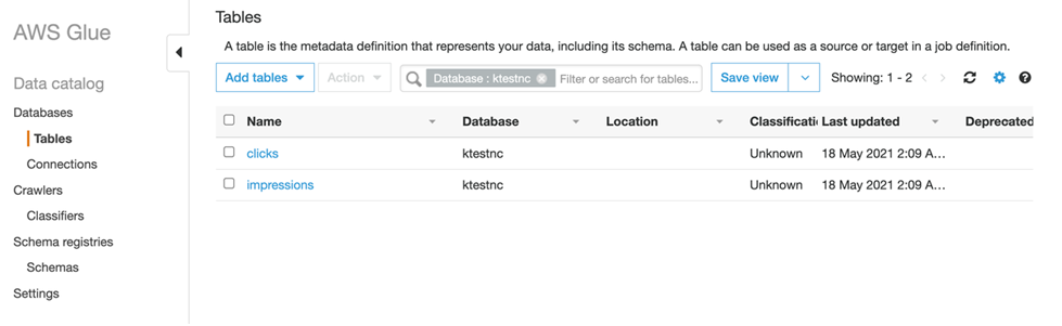
The following screenshot is the AWS Glue Data Catalog view, which shows the tables that represent MSK topics.

In the preceding tables, WATERMARK FOR serve_time AS serve_time - INTERVAL '5' SECOND means that we can tolerate out-of-order delivery of events in the timeframe of 5 seconds and still produce correct results.

After you create the tables, run a query that calculates the number of impressions within a tumbling window of 60 seconds broken down by campaign_id and creative_details:

%flink.ssql(type=update)
SELECT 
 campaign_id, 
 creative_details, 
 TUMBLE_ROWTIME(serve_time, INTERVAL '60' SECOND) 
   AS window_end, COUNT(*) AS c
FROM impressions
GROUP BY 
  TUMBLE(serve_time, INTERVAL '60' SECOND), 
  campaign_id, 
  creative_details
ORDER BY window_end, c DESC;

The results from this query appear as soon as results are available.

Additionally, we want to see the clickthrough rate of the impressions:

SELECT 
  bid_id, 
  campaign_id,
  country_code, 
  creative_details, 
  CAST(serve_time AS TIMESTAMP) AS serveTime, 
  tracker,
  CAST(click_time AS TIMESTAMP) AS clickTime,
  CASE
     WHEN `click_time` IS NULL THEN FALSE
     WHEN `click_time` IS NOT NULL THEN TRUE
  END AS clicked
FROM  impressions 
LEFT OUTER JOIN clicks 
  ON bid_id = correlation_id AND
  click_time BETWEEN  serve_time AND 
  serve_time + INTERVAL '2' MINUTE ;

This query produces one row for each impression and matches it with a click (if any) that was observed within 2 minutes after serving the ad. This is essentially performing a join operation across the topics to get this information.

You can insert this data back into an existing Kafka topic using the following code:

INSERT INTO clickthroughrate 
SELECT 
  bid_id, 
  campaign_id,
  country_code, 
  creative_details, 
  CAST(serve_time AS TIMESTAMP WITHOUT TIME ZONE) AS serveTime, 
  tracker,
  CAST(click_time AS TIMESTAMP WITHOUT TIME ZONE) AS clickTime,
  CASE
     WHEN `click_time` IS NULL THEN FALSE
     WHEN `click_time` IS NOT NULL THEN TRUE
  END AS clicked
FROM  impressions 
LEFT OUTER JOIN clicks 
  ON bid_id = correlation_id AND
  click_time BETWEEN  serve_time AND 
  serve_time + INTERVAL '2' MINUTE ;

Create the corresponding table for the Kafka topic in the Data Catalog if it doesn’t exist already. After you run the preceding query, you can see data in your Amazon MSK topic (see the following sample below):

1095810839,1911670336,KH,"mint green","2021-06-15 01:08:00","ainhpsm6vxgs4gvyl52v13s173gntd7jyitlq328qmam37rpbs2tj1il049dlyb2vgwx89dbvwezl2vkcynqvlqfql7pxp8blg6807yxy1y54eedwff2nuhrbqhce36j00mbxdh72fpjmztymobq79y1g3xoyr6f09rgwqna1kbejkjw4nfddmm0d56g3mkd8obrrzo81z0ktu934a00b04e9q0h1krapotnon76rk0pmw6gr8c24wydp0b2yls","2021-06-15 01:08:07",true
0946058105,1913684520,GP,magenta,"2021-06-15 01:07:56","7mlkc1qm9ntazr7znfn9msew75xs9tf2af96ys8638l745t2hxwnmekaft735xdcuq4xtynpxr68orw5gmbrhr9zyevhawjwfbvzhlmziao3qs1grsb5rdzysvr5663qg2eqi5p7braruyb6rhyxkf4x3q5djo7e1jd5t91ybop0cxu4zqmwkq7x8l7c4y33kd4gwd4g0jmm1hy1df443gdq5tnj8m1qaymr0q9gatqt7jg61cznql0z6ix8pyr","2021-06-15 01:08:07",true
0920672086,0888784120,CK,silver,"2021-06-15 01:08:03","gqr76xyhu2dmtwpv9k3gxihvmn7rluqblh39gcrfyejt0w8jwwliq24okxkho1zuyxdw9mp4vzwi0nd4s5enhvm2d74eydtqnmf7fm4jsyuhauhh3d32esc8gzpbwkgs8yymlp22ih6kodrpjj2bayh4bjebcoeb42buzb43ii1e0zv19bxb8suwg17ut2mdhj4vmf8g9jl02p2tthe9w3rpv7w9w16d14bstiiviy4wcf86adfpz378a49f36q","2021-06-15 01:08:16",true

This is the CSV data from the preceding query, which shows the ClickThroughRate for the impressions. You can use this mechanism to store data back persistently into Kafka from Flink directly.

Scala

We use the %flink header to signify that this code block will be interpreted via the Scala Flink interpreter, and create a table identical to the one from the SQL example. However, in this example, we use the Scala interpreter’s built-in streaming table environment variable, stenv, to run a SQL DDL statement. If the table already exists in the AWS Glue Data Catalog, this statement issues an error stating that the table already exists.

%flink 
stenv.executeSql("""CREATE TABLE impressions (
  bid_id VARCHAR,
  creative_details VARCHAR(10),
  campaign_id VARCHAR,
  country_code VARCHAR(5),
  i_timestamp VARCHAR,
  serve_time as TO_TIMESTAMP (`i_timestamp`, 'EEE MMM dd HH:mm:ss z yyyy'),
  WATERMARK FOR serve_time AS serve_time -INTERVAL '5' SECOND
  )
  WITH (
  'connector'= 'kafka',
  'topic' = 'impressions',
  'properties.bootstrap.servers' = '< Bootstrap Servers shown in the MSK client info dialog >',
  'format' = 'json',
  'properties.group.id' = 'testGroup1',
  'scan.startup.mode'= 'earliest-offset',
  'json.timestamp-format.standard'= 'ISO-8601'
  )""")

stenv.executeSql("""
 CREATE TABLE clicks (
 correlation_id VARCHAR,
 tracker VARCHAR(100),
 c_timestamp VARCHAR,
 click_time as TO_TIMESTAMP (`c_timestamp`, 'EEE MMM dd HH:mm:ss z yyyy'),
 WATERMARK FOR click_time AS click_time -INTERVAL '5' SECOND
 )
 WITH (
 'connector'= 'kafka',
 'topic' = 'clicks',
 'properties.bootstrap.servers' = '< Bootstrap Servers shown in the MSK client info dialog >',
 'format' = 'json',
 'properties.group.id' = 'testGroup1',
 'scan.startup.mode'= 'earliest-offset',
 'json.timestamp-format.standard'= 'ISO-8601'
 )""")

Performing a tumbling window in the Scala table API first requires the definition of an in-memory reference to the table we created. We use the stenv variable to define this table using the from function and referencing the table name. After this is created, we can create a windowed aggregation over 1 minute of data, serve_time column. See the following code:

%flink
val inputTable: Table = stenv.from("impressions")
val tumblingWindowTable = inputTable.window(Tumble over 1.minute on $"serve_time" as $"oneMinuteWindow")
.groupBy( $"oneMinuteWindow", $"campaign_id",$"creative_details")
.select($"campaign_id", $"creative_details", $"oneMinuteWindow".rowtime as "window_end",$"creative_details".count as "c")

Use the ZeppelinContext to visualize the Scala table aggregation within the notebook:

%flink
z.show(tumblingWindowTable, streamType="update")

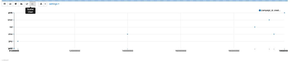
The following screenshot shows our results.

Additionally, we want to see the clickthrough rate of the impressions by joining with the clicks:

val left:Table = stenv.from("impressions").select("bid_id,campaign_id,country_code,creative_details,serve_time")
val right:Table = stenv.from("clicks").select("correlation_id,tracker,click_time")
val result:Table = left.leftOuterJoin(right).where($"bid_id" === $"correlation_id" && $"click_time" < ( $"serve_time" + 2.minutes) && $"click_time" > $"serve_time").select($"bid_id", $"campaign_id", $"country_code",$"creative_details",$"tracker",$"serve_time".cast(Types.SQL_TIMESTAMP) as "s_time", $"click_time".cast(Types.SQL_TIMESTAMP) as "c_time" , $"click_time".isNull.?("false","true") as "clicked" )

Use the ZeppelinContext to visualize the Scala table aggregation within the notebook.

z.show(result, streamType="update")

The following screenshot shows our results.

Python

We use the %flink.pyflink header to signify that this code block will be interpreted via the Python Flink interpreter, and create a table identical to the one from the SQL and Scala examples. In this example, we use the Python interpreter’s built-in streaming table environment variable, st_env, to run a SQL DDL statement. If the table already exists in the AWS Glue Data Catalog, this statement issues an error stating that the table already exists.

%flink.pyflink
st_env.execute_sql("""
 CREATE TABLE impressions (
 bid_id VARCHAR,
 creative_details VARCHAR(10),
 campaign_id VARCHAR,
 country_code VARCHAR(5),
 i_timestamp VARCHAR,
 serve_time as TO_TIMESTAMP (`i_timestamp`, 'EEE MMM dd HH:mm:ss z yyyy'),
 WATERMARK FOR serve_time AS serve_time -INTERVAL '5' SECOND
 )
 WITH (
 'connector'= 'kafka',
 'topic' = 'impressions',
 'properties.bootstrap.servers' = '< Bootstrap Servers shown in the MSK client info dialog >',
 'format' = 'json',
 'properties.group.id' = 'testGroup1',
 'scan.startup.mode'= 'earliest-offset',
 'json.timestamp-format.standard'= 'ISO-8601'
 )""")
 
st_env.execute_sql("""
 CREATE TABLE clicks (
 correlation_id VARCHAR,
 tracker VARCHAR(100),
 c_timestamp VARCHAR,
 click_time as TO_TIMESTAMP (`c_timestamp`, 'EEE MMM dd HH:mm:ss z yyyy'),
 WATERMARK FOR click_time AS click_time -INTERVAL '5' SECOND
 )
 WITH (
 'connector'= 'kafka',
 'topic' = 'clicks',
 'properties.bootstrap.servers' = '< Bootstrap Servers shown in the MSK client info dialog >',
 'format' = 'json',
 'properties.group.id' = 'testGroup1',
 'scan.startup.mode'= 'earliest-offset',
 'json.timestamp-format.standard'= 'ISO-8601'
 )""")

Performing a sliding (hopping) window in the Python table API first requires the definition of an in-memory reference to the table we created. We use the st_env variable to define this table using the from_path function and referencing the table name. After this is created, we can create a windowed aggregation over 1 minute of data, emitting results every 5 seconds according to the event_time column. See the following code:

%flink.pyflink

input_table = st_env.from_path("impressions")
tumbling_window_table =(input_table.window(Tumble.over("1.minute").on("serve_time").alias("one_minute_window"))
.group_by( "one_minute_window, campaign_id, creative_details")
.select("campaign_id, creative_details, one_minute_window.end as window_end, creative_details.count as c"))

Use the ZeppelinContext to visualize the Python table aggregation within the notebook:

%flink.pyflink

z.show(tumbling_window_table, stream_type="update")

The following screenshot shows our results.

Additionally, we want to see the clickthrough rate of the impressions by joining with the clicks:

impressions = st_env.from_path("impressions").select("bid_id,campaign_id,country_code,creative_details,serve_time")
clicks = st_env.from_path("clicks").select("correlation_id,tracker,click_time")
results = impressions.left_outer_join(clicks).where("bid_id == correlation_id && click_time < (serve_time + 2.minutes) && click_time > serve_time").select("bid_id, campaign_id, country_code, creative_details, tracker, serve_time.cast(STRING) as s_time, click_time.cast(STRING) as c_time, (click_time.isNull).?('false','true') as clicked")

Scaling

A Studio notebook consists of one or more tasks. You can split a Studio notebook task into several parallel instances to run, where each parallel instance processes a subset of the task’s data. The number of parallel instances of a task is called its parallelism, and adjusting that helps run your tasks more efficiently.

On creation, Studio notebooks are given four parallel Kinesis Processing Units (KPUs), which make up the application parallelism. To increase that parallelism, navigate to the Kinesis Data Analytics console, choose your application name, and choose the Configuration tab.

From this page, in the Scaling section, choose Edit and modify the Parallelism entry. We don’t recommend increasing the Parallelism Per KPU setting higher than 1 unless your application is I/O bound.

Choose Save changes to increase or decrease your application’s parallelism.

Clean up

You may want to clean up the demo environment when you are done, To do so, stop the Studio notebook and delete the resources created for the Data Generator and the Amazon MSK cluster ( if you created a new cluster).

Summary

Kinesis Data Analytics Studio makes developing stream processing applications using Apache Flink much faster, with rich visualizations, a scalable and user-friendly interface to develop pipelines, and the flexibility of language choice to make any streaming workload performant and powerful. You can run paragraphs from within the notebook or promote your Studio notebook to a Kinesis Data Analytics for Apache Flink application with a durable state, as shown in the SQL example in this post.

For more information, see the following resources:

• Amazon Kinesis Data Analytics features
• Using a Studio notebook with Kinesis Data Analytics for Apache Flink
• Apache Flink Documentation
• Flink interpreter for Apache Zeppelin

About the Author

Chinmayi Narasimhadevara is a Solutions Architect focused on Big Data and Analytics at Amazon Web Services. Chinmayi has over 15 years of experience in information technology. She helps AWS customers build advanced, highly scalable and performant solutions