Post Syndicated from Paul Villena original https://aws.amazon.com/blogs/big-data/build-near-real-time-logistics-dashboards-using-amazon-redshift-and-amazon-managed-grafana-for-better-operational-intelligence/

Amazon Redshift is a fully managed data warehousing service that is currently helping tens of thousands of customers manage analytics at scale. It continues to lead price-performance benchmarks, and separates compute and storage so each can be scaled independently and you only pay for what you need. It also eliminates data silos by simplifying access to your operational databases, data warehouse, and data lake with consistent security and governance policies.

With the Amazon Redshift streaming ingestion feature, it’s easier than ever to access and analyze data coming from real-time data sources. It simplifies the streaming architecture by providing native integration between Amazon Redshift and the streaming engines in AWS, which are Amazon Kinesis Data Streams and Amazon Managed Streaming for Apache Kafka (Amazon MSK). Streaming data sources like system logs, social media feeds, and IoT streams can continue to push events to the streaming engines, and Amazon Redshift simply becomes just another consumer. Before Amazon Redshift streaming was available, we had to stage the streaming data first in Amazon Simple Storage Service (Amazon S3) and then run the copy command to load it into Amazon Redshift. Eliminating the need to stage data in Amazon S3 results in faster performance and improved latency. With this feature, we can ingest hundreds of megabytes of data per second and have a latency of just a few seconds.

Another common challenge for our customers is the additional skill required when using streaming data. In Amazon Redshift streaming ingestion, only SQL is required. We use SQL to do the following:

• Define the integration between Amazon Redshift and our streaming engines with the creation of external schema
• Create the different streaming database objects that are actually materialized views
• Query and analyze the streaming data
• Generate new features that are used to predict delays using machine learning (ML)
• Perform inferencing natively using Amazon Redshift ML

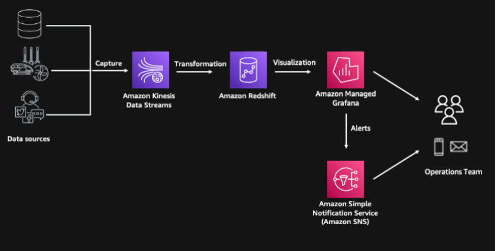
In this post, we build a near real-time logistics dashboard using Amazon Redshift and Amazon Managed Grafana. Our example is an operational intelligence dashboard for a logistics company that provides situational awareness and augmented intelligence for their operations team. From this dashboard, the team can see the current state of their consignments and their logistics fleet based on events that happened only a few seconds ago. It also shows the consignment delay predictions of an Amazon Redshift ML model that helps them proactively respond to disruptions before they even happen.

Solution overview

This solution is composed of the following components, and the provisioning of resources is automated using the AWS Cloud Development Kit (AWS CDK):

• Multiple streaming data sources are simulated through Python code running in our serverless compute service, AWS Lambda
• The streaming events are captured by Amazon Kinesis Data Streams, which is a highly scalable serverless streaming data service
• We use the Amazon Redshift streaming ingestion feature to process and store the streaming data and Amazon Redshift ML to predict the likelihood of a consignment getting delayed
• We use AWS Step Functions for serverless workflow orchestration
• The solution includes a consumption layer built on Amazon Managed Grafana where we can visualize the insights and even generate alerts through Amazon Simple Notification Service (Amazon SNS) for our operations team

The following diagram illustrates our solution architecture.

Prerequisites

The project has the following prerequisites:

• An AWS account.
• Amazon Linux 2 with AWS CDK, Docker CLI, and Python3 installed. Alternatively, setting up an AWS Cloud9 environment will satisfy this requirement.
• To run this code, you need elevated privileges into the AWS account you are using.

Sample deployment using the AWS CDK

The AWS CDK is an open-source project that allows you to define your cloud infrastructure using familiar programming languages. It uses high-level constructs to represent AWS components to simplify the build process. In this post, we use Python to define the cloud infrastructure due to its familiarity to many data and analytics professionals.

Clone the GitHub repository and install the Python dependencies:

git clone https://github.com/aws-samples/amazon-redshift-streaming-workshop
cd amazon-redshift-streaming-workshop
python3 -m venv .venv
source .venv/bin/activate
pip install -r requirements.txt

Next, bootstrap the AWS CDK. This sets up the resources required by the AWS CDK to deploy into the AWS account. This step is only required if you haven’t used the AWS CDK in the deployment account and Region.

cdk bootstrap

Deploy all stacks:

cdk deploy IngestionStack 
cdk deploy RedshiftStack 
cdk deploy StepFunctionStack

The entire deployment time takes 10–15 minutes.

Access streaming data using Amazon Redshift streaming ingestion

The AWS CDK deployment provisions an Amazon Redshift cluster with the appropriate default IAM role to access the Kinesis data stream. We can create an external schema to establish a connection between the Amazon Redshift cluster and the Kinesis data stream:

CREATE EXTERNAL SCHEMA ext_kinesis FROM KINESIS
IAM_ROLE default;

For instructions on how to connect to the cluster, refer to Connecting to the Redshift Cluster.

We use a materialized view to parse data in the Kinesis data stream. In this case, the whole payload is ingested as is and stored using the SUPER data type in Amazon Redshift. Data stored in streaming engines is usually in semi-structured format, and the SUPER data type provides a fast and efficient way to analyze semi-structured data within Amazon Redshift.

See the following code:

CREATE MATERIALIZED VIEW consignment_stream AS
SELECT approximate_arrival_timestamp,
JSON_PARSE(from_varbyte(kinesis_data, 'utf-8')) as consignment_data FROM ext_kinesis.consignment_stream
WHERE is_utf8(kinesis_data)
AND is_valid_json(from_varbyte(kinesis_data, 'utf-8'));

Refreshing the materialized view invokes Amazon Redshift to read data directly from the Kinesis data stream and load it into the materialized view. This refresh can be done automatically by adding the AUTO REFRESH clause in the materialized view definition. However, in this example, we are orchestrating the end-to-end data pipeline using AWS Step Functions.

REFRESH MATERIALIZED VIEW consignment_stream;

Now we can start running queries against our streaming data and unify it with other datasets like logistics fleet data. If we want to know the distribution of our consignments across different states, we can easily unpack the contents of the JSON payload using the PartiQL syntax.

SELECT cs.consignment_data.origin_state::VARCHAR,
COUNT(1) number_of_consignments,
AVG(on_the_move) running_fleet,
AVG(scheduled_maintenance + unscheduled_maintenance) under_maintenance
FROM consignment_stream cs
INNER JOIN fleet_summary fs
on TRIM(cs.consignment_data.origin_state::VARCHAR) = fs.vehicle_location
GROUP BY 1

Generate features using Amazon Redshift SQL functions

The next step is to transform and enrich the streaming data using Amazon Redshift SQL to generate additional features that will be used by Amazon Redshift ML for its predictions. We use date and time functions to identify the day of the week, and calculate the number of days between the order date and target delivery date.

We also use geospatial functions, specifically ST_DistanceSphere, to calculate the distance between origin and destination locations. The GEOMETRY data type within Amazon Redshift provides a cost-effective way to analyze geospatial data such as longitude and latitudes at scale. In this example, the addresses have already been converted to longitude and latitude. However, if you need to perform geocoding, you can integrate Amazon Location Services with Amazon Redshift using user-defined functions (UDFs). On top of geocoding, Amazon Location Service also allows you to more accurately calculate route distance between origin and destination, and even specify waypoints along the way.

We use another materialized view to persist these transformations. A materialized view provides a simple yet efficient way to create data pipelines using its incremental refresh capability. Amazon Redshift identifies the incremental changes from the last refresh and only updates the target materialized view based on these changes. In this materialized view, all our transformations are deterministic, so we expect our data to be consistent when going through a full refresh or an incremental refresh.

See the following code:

CREATE MATERIALIZED VIEW consignment_transformed AS
SELECT
consignment_data.consignmentid::INT consignment_id,
consignment_data.consignment_date::TIMESTAMP consignment_date,
consignment_data.delivery_date::TIMESTAMP delivery_date,
consignment_data.origin_state::VARCHAR origin_state,
consignment_data.destination_state::VARCHAR destination_state,
consignment_data.revenue::FLOAT revenue,
consignment_data.cost::FLOAT cost,
DATE_PART(dayofweek, consignment_data.consignment_date::TIMESTAMP)::INT day_of_week,
DATE_PART(hour, consignment_data.consignment_date::TIMESTAMP)::INT "hour",
DATEDIFF(days,
consignment_data.consignment_date::TIMESTAMP,
consignment_data.delivery_date::TIMESTAMP
)::INT days_to_deliver,
(ST_DistanceSphere(
ST_Point(consignment_data.origin_lat::FLOAT, consignment_data.origin_long::FLOAT),
ST_Point(consignment_data.destination_lat::FLOAT, consignment_data.destination_long::FLOAT)
) / 1000 --convert to km
) delivery_distance
FROM consignment_stream;

Predict delays using Amazon Redshift ML

We can use this enriched data to make predictions on the delay probability of a consignment. Amazon Redshift ML is a feature of Amazon Redshift that allows you to use the power of Amazon Redshift to build, train, and deploy ML models directly within your data warehouse.

The training of a new Amazon Redshift ML model has been initiated as part of the AWS CDK deployment using the CREATE MODEL statement. The training dataset is defined in the FROM clause, and TARGET defines which column the model is trying to predict. The FUNCTION clause defines the name of the function that is used to make predictions.

CREATE MODEL ml_delay_prediction -- already executed by CDK
FROM (SELECT * FROM ext_s3.consignment_train)
TARGET probability
FUNCTION fnc_delay_probabilty
IAM_ROLE default
SETTINGS (
MAX_RUNTIME 1800, --seconds
S3_BUCKET '<ingestionstack-s3bucketname>' --replace S3 bucket name
)

This simplified model is trained using historical observations, and the training process takes around 30 minutes to complete. You can check the status of the training job by running the SHOW MODEL statement:

SHOW MODEL ml_delay_prediction;

When the model is ready, we can start making predictions on new data that is streamed into Amazon Redshift. Predictions are generated using the Amazon Redshift ML function that was defined during the training process. We pass the calculated features from the transformed materialized view into this function, and the prediction results populate the delay_probability column.

This final output is persisted into the consignment_predictions table, and Step Functions is orchestrating the ongoing incremental data load into this target table. We use a table for the final output, instead of a materialized view, because ML predictions have randomness involved and it may give us non-deterministic results. Using a table gives us more control on how data is loaded.

See the following code:

CREATE TABLE consignment_predictions AS
SELECT *, fnc_delay_probability(
day_of_week, "hour", days_to_deliver, delivery_distance) delay_probability
FROM consignment_transformed;

Create an Amazon Managed Grafana dashboard

We use Amazon Managed Grafana to create a near real-time logistics dashboard. Amazon Managed Grafana is a fully managed service that makes it easy to create, configure, and share interactive dashboards and charts for monitoring your data. We can also use Grafana to set up alerts and notifications based on specific conditions or thresholds, allowing you to quickly identify and respond to issues.

The high-level steps in setting up the dashboard are as follows:

1. Create a Grafana workspace.
2. Set up Grafana authentication using AWS IAM Identity Center (successor to AWS Single Sign-On) or using direct SAML integration.
3. Configure Amazon Redshift as a Grafana data source.
4. Import the JSON file for the near real-time logistics dashboard.

A more detailed set of instructions is available in the GitHub repository for your reference.

Clean up

To avoid ongoing charges, delete the resources deployed. Access the Amazon Linux 2 environment and run the AWS CDK destroy command. Delete the Grafana objects related to this deployment.

cd amazon-redshift-streaming-workshop
source .venv/bin/activate
cdk destroy –all

Conclusion

In this post, we showed how easy it is to build a near real-time logistics dashboard using Amazon Redshift and Amazon Managed Grafana. We created an end-to-end modern data pipeline using only SQL. This shows how Amazon Redshift is a powerful platform for democratizing your data—it enables a wide range of users, including business analysts, data scientists, and others, to work with and analyze data without requiring specialized technical skills or expertise.

We encourage you to explore what else can be achieved with Amazon Redshift and Amazon Managed Grafana. We also recommend you visit the AWS Big Data Blog for other useful blog posts on Amazon Redshift.

About the Author

Paul Villena is an Analytics Solutions Architect in AWS with expertise in building modern data and analytics solutions to drive business value. He works with customers to help them harness the power of the cloud. His areas of interests are infrastructure-as-code, serverless technologies and coding in Python.