Tag Archives: Kinesis Data Streams

Amazon Kinesis Data Streams launches On-demand Advantage for instant throughput increases and streaming at scale

Post Syndicated from Pratik Patel original https://aws.amazon.com/blogs/big-data/amazon-kinesis-data-streams-launches-on-demand-advantage-for-instant-throughput-increases-and-streaming-at-scale/

Today, AWS announced the new Amazon Kinesis Data Streams On-demand Advantage mode, which includes warm throughput capability and an updated pricing structure. With this feature you can enable instant scaling for traffic surges while optimizing costs for consistent streaming workloads. On-demand Advantage mode is a cost-effective way to stream with Kinesis Data Streams for use cases that ingest at least 10 MiB/s in aggregate or have hundreds of data streams in an AWS Region.

In this post, we explore this new feature, including key use cases, configuration options, pricing considerations, and best practices for optimal performance.

Real-world use cases

As streaming data volumes grow and use cases evolve, you can face two common challenges with your streaming workloads:

Challenge 1: Preparing for traffic spikes

Many businesses experience predictable but significant traffic surges during events like product launches, content releases, or holiday sales. Using an on-demand capacity mode, you have to complete several steps when preparing for traffic spikes:

  • Transition to provisioned mode
  • Manually estimate and increase shards based on anticipated peak demand
  • Wait for scaling operations to finish
  • Subsequently return to on-demand mode

This mode-switching process was time consuming, required careful planning, and introduced operational complexity, forcing customers to either accept this operational burden, overprovision capacity well in advance, or risk throttling during critical business periods when data ingestion reliability matters most.

Challenge 2: Cost optimization for consistent workloads

Organizations with large, consistent streaming workloads want to optimize costs without sacrificing the simplicity and scalability available with on-demand streams. On-demand capacity mode serves well for fluctuating data traffic, yet customers desired a more economical approach to handle high-volume streaming workloads.

On-demand Advantage directly address both challenges by providing the capability to warm on-demand streams and a new pricing structure. With the new On-demand Advantage mode, there is no longer a fixed, per-stream charge, and the throughput usage is priced at a lower rate. The only requirement is that the account commits to streaming with at least 25 MiB/s of data ingest and 25 MiB/s of data retrieval usage.

This launch improves data streaming across multiple industries:

  • Online gaming companies can now prepare their streams for game launches without the cumbersome process of switching between modes and manually calculating shard requirements
  • Media and entertainment providers can support smooth data ingestion during major content releases and live events
  • E-commerce services can handle holiday sales traffic while optimizing costs for their baseline workloads.

By combining instant scaling with cost efficiency, you can confidently manage both predictable traffic surges and consistent streaming volumes without compromising on performance or budget.

How it works

The key features of On-demand Advantage mode are warm throughput and committed-usage pricing.

Warm throughput

With the warm throughput feature, available once you’ve enabled On-demand Advantage mode, you can configure your Kinesis Data Streams on-demand streams to have instantly available throughput capacity up to 10 GiB/s. This means you can proactively prepare on-demand streams for expected peak traffic events without the cumbersome process of switching between provisioned modes and manually calculating shard requirements. Key benefits include:

  • The ability to prepare for peak events so you can handle traffic surges smoothly
  • Alleviation of the need to build custom scaling solutions
  • The capability to continue scaling automatically beyond warm throughput if needed, up to 10 GiB/s or 10 million events per second
  • No additional fee for maintaining warm capacity

Committed-usage pricing

When you’ve enabled On-demand Advantage mode, the billing for the on-demand streams switches to a new structure that removes the stream hour charge and offers a discount of at least 60% for the throughput usage. Based on US East (N. Virginia) pricing, data ingested is priced 60% lower, data retrieval is priced 60% lower, Enhanced fan-out data retrieval is 68% lower, and extended retention is priced 77% lower. In return, you commit to stream 25 MiB/s for at least 24 hours. Even when actual usage is lower, if you enable this setting, you’re charged for the minimum 25 MiB/s throughput at the discounted price. Overall, the signficant discounts offered means that On-demand Advantage is more cost-effective for use cases that ingest at least 10 MiB/s in aggregate, fan out to more than two consumer applications, or have hundreds of data streams in an AWS Region.

Getting started

Follow these steps to start using On-demand Advantage mode.

Enabling On-demand Advantage mode

To start using the On-demand Advantage mode:

In the AWS Management Console

  1. Navigate to the Kinesis Data Streams console
  2. Navigate to the Account Settings tab
  3. Choose Edit billing mode
  4. Select the On-demand Advantage option
  5. Select the checkbox, I acknowledge this change cannot be reverted for 24 hours
  6. Choose Save changes

on-demand-billing-mode

Using the AWS CLI

You can run the following CLI command to enable the minimum throughput billing commitment:

aws kinesis update-account-settings \
--minimum-throughput-billing-commitment Status=ENABLED

Using the AWS SDK

You can use the SDK to enable the minimum throughput billing commitment. The following Python example shows how to do it:

import boto3

client = boto3.client('kinesis')
response = client.update_account_settings(
    MinimumThroughputBillingCommitment={"Status": "ENABLED"}
)

Once enabled, you commit your stream to this pricing mode for a minimum period of 24 hours, after which you can opt out as needed.

Configuring warm throughput

To start using warm throughput for Kinesis Data Streams On-demand:

Using the AWS Management Console

  1. Navigate to the Kinesis Data Streams console
  2. Select your stream and go to the Configuration tab
  3. Choose Edit next to Warm Throughput
  4. Set your desired warm throughput (up to 10 GiB/s)
  5. Save your changes

Using the AWS CLI

You can run the following CLI command to enable the warm throughput:

aws kinesis update-stream-warm-throughput \
  --stream-name MyStream \
  --warm-throughput-mi-bps 1000

Using the AWS SDK:

You can use the SDK to enable warm throughput. The following Python example shows how to do it:

import boto3

client = boto3.client('kinesis')
response = client.update_stream_warm_throughput(
    StreamName='MyStream',
    WarmThroughputMiBps=1000
)

You can also create a new on-demand stream with warm throughput using the existing CreateStream API, or set warm throughput when converting a data stream from provisioned to On-demand Advantage mode.

Throttling and best practices for optimal performance

When working with warm throughput, it’s important to understand how capacity is managed. Each stream can instantly handle traffic up to the configured warm throughput level and will automatically scale beyond that as needed.

For optimal performance with warm throughput:

  1. Use a uniformly distributed partition key strategy to evenly distribute records across shards and avoid hotspots and consider your partition key strategy carefully as you can ingest a maximum of 1 MiB/s of data per partition key, regardless of the warm throughput configured.
  2. Monitor throughput metrics to adjust warm throughput settings based on actual usage patterns.
  3. Implement backoff and retry logic in producer applications to handle potential throttling.

For cost optimization with committed usage pricing:

  1. Analyze your daily throughput to verify it is at least 10 MiB/s.
  2. Consider consolidating streams across your organization to maximize the benefit of the discount for on-demand streams.
  3. Use cost effective data retrievals with – Use Enhanced Fan-Out – Use Enhanced Fan-Out consumers for applications that need dedicated throughput with 68% lower data retrievals cost in advantage mode.

Warm throughput in action

To demonstrate how warm throughput behaves, we enabled committed pricing in an AWS account and created two on-demand streams: “KDS-OD-STANDARD” and “KDS-OD-WARM-TP”. The “KDS-OD-WARM-TP” stream was configured with 100 MiB/second warm throughput, while “KDS-OD-STANDARD” remained as a regular on-demand stream without warm throughput, as demonstrated in the following screenshot.

od-standard-warm-streams

In our experiment, we initially simulated approximately 2 MiB/second traffic ingest for both “KDS-OD-STANDARD” and “KDS-OD-WARM-TP” streams. We used a UUID as a partition key so that traffic was evenly distributed across the shards of the Kinesis data streams, helping prevent potential hotspots that might skew our results. After establishing this baseline, we increased the ingest traffic to around 28 MiB/second within 10 minutes. We then further escalated the traffic to exceed 60 MiB/second within 15 minutes of the initial increase, as illustrated in the following screenshot.

streams-ingest-mb-second-metric

The following graph shows the ThrottledRecords CloudWatch metric for both “KDS-OD-STANDARD” and “KDS-OD-WARM-TP” that the warm throughput-enabled stream (“KDS-OD-WARM-TP”) did not encounter throttles during both traffic spikes, as it had 100 MiB/second warm throughput configured. In contrast, the standard on-demand stream (“KDS-OD-STANDARD”) experienced throttling when we increased traffic by 14x initially and by 2x later, before eventually scaling to bring throttles back to zero. This experiment demonstrates that you can use warm throughput to instantly prepare for peak usage times and avoid throttling during sudden traffic increases.

streams-throttle-metrics

Conclusion

As we outlined in this post, the new Amazon Kinesis Data Streams On-demand Advantage mode provides significant benefits for organizations of different sizes:

  • Instant scaling for predictable traffic surges without overprovisioning.
  • Cost optimization for consistent streaming workloads with at least 60% discount.
  • Simplified operations with no need to switch between different capacity modes.
  • Enhanced flexibility to handle both expected and unexpected traffic patterns.

With these enhancements you can build and operate real-time streaming applications at many scales. Kinesis Data Streams now provides the ideal combination of scalability, performance, and cost-efficiency.

To learn more about these new features, visit the Amazon Kinesis Data Streams documentation.


About the authors

Roy (KDS) Wang

Roy (KDS) Wang

Roy is a Senior Product Manager with Amazon Kinesis Data Streams. He is passionate about learning from and collaborating with customers to help organizations run faster and smarter. Outside of work, Roy strives to be a good dad to his new son and builds plastic model kits.

Pratik Patel

Pratik Patel

Pratik is Sr. Technical Account Manager and streaming analytics specialist. He works with AWS customers and provides ongoing support and technical guidance to help plan and build solutions using best practices and proactively keep customers’ AWS environments operationally healthy.

Umesh Chaudhari

Umesh Chaudhari

Umesh is a Sr. Streaming Solutions Architect at AWS. He works with customers to design and build real-time data processing systems. He has extensive working experience in software engineering, including architecting, designing, and developing data analytics systems. Outside of work, he enjoys traveling, following tech trends.

Simon Peyer

Simon Peyer

Simon is a Solutions Architect at AWS based in Switzerland. He is a practical doer and passionate about connecting technology and people using AWS Cloud services. A special focus for him is data streaming and automations. Besides work, Simon enjoys his family, the outdoors, and hiking in the mountains.20

Amazon Kinesis Data Streams now supports 10x larger record sizes: Simplifying real-time data processing

Post Syndicated from Sumant Nemmani original https://aws.amazon.com/blogs/big-data/amazon-kinesis-data-streams-now-supports-10x-larger-record-sizes-simplifying-real-time-data-processing/

Today, AWS announced that Amazon Kinesis Data Streams now supports record sizes up to 10MiB – a tenfold increase from the previous limit. With this launch, you can now publish intermittent larger data payloads on your data streams while continuing to use existing Kinesis Data Streams APIs in your applications without additional effort. This launch is accompanied by a 2x increase in the maximum PutRecords request size from 5MiB to 10MiB, simplifying data pipelines and reducing operational overhead for IoT analytics, change data capture, and generative AI workloads.

In this post, we explore Amazon Kinesis Data Streams large record support, including key use cases, configuration of maximum record sizes, throttling considerations, and best practices for optimal performance.

Real world use cases

As data volumes grow and use cases evolve, we’ve seen increasing demand for supporting larger record sizes in streaming workloads. Previously, when you needed to process records larger than 1MiB, you had two options:

  • Split large records into multiple smaller records in producer applications and reassemble them in consumer applications
  • Store large records in Amazon Simple Storage Service (Amazon S3) and send only metadata through Kinesis Data Streams

Both these approaches are useful, but they add complexity to data pipelines, requiring additional code, increasing operational overhead, and complicating error handling and debugging, particularly when customers need to stream large records intermittently.

This enhancement improves the ease of use and reduces operational overhead for customers handling intermittent data payloads across various industries and use cases. In the IoT analytics domain, connected vehicles and industrial equipment are generating increasing volumes of sensor telemetry data, with the size of individual telemetry records occasionally exceeding the previous 1MiB limit in Kinesis. This required customers to implement complex workarounds, such as splitting large records into multiple smaller ones or storing the large records separately and only sending metadata through Kinesis. Similarly, in database change data capture (CDC) pipelines, large transaction records can be produced, especially during bulk operations or schema changes. In the machine learning and generative AI space, workflows are increasingly requiring the ingestion of larger payloads to support richer feature sets and multi-modal data types like audio and images. The increased Kinesis record size limit from 1MiB to 10MiB limits the need for these types of complex workarounds, simplifying data pipelines and reducing operational overhead for customers in IoT, CDC, and advanced analytics use cases. Customers can now more easily ingest and process these intermittent large data records using the same familiar Kinesis APIs.

How it works

To start processing larger records:

  1. Update your stream’s maximum record size limit (maxRecordSize) through the AWS Console, AWS CLI, or AWS SDKs.
  2. Continue using the same PutRecord and PutRecords APIs for producers.
  3. Continue using the same GetRecords or SubscribeToShard APIs for consumers.

Your stream will be in Updating status for a few seconds before being ready to ingest larger records.

Getting started

To start processing larger records with Kinesis Data Streams, you can update the maximum record size by using the AWS Management Console, CLI or SDK.

On the AWS Management Console,

  1. Navigate to the Kinesis Data Streams console.
  2. Choose your stream and select the Configuration tab.
  3. Choose Edit (next to Maximum record size).
  4. Set your desired maximum record size (up to 10MiB).
  5. Save your changes.

Note: This setting only adjusts the maximum record size for this Kinesis data stream. Before increasing this limit, verify that all downstream applications can handle larger records.

Most common consumers such as Kinesis Client Library (starting with version 2.x), Amazon Data Firehose delivery to Amazon S3 and AWS Lambda support processing records larger than 1 MiB. To learn more, refer to the Amazon Kinesis Data Streams documentation for large records.

You can also update this setting using the AWS CLI:

aws kinesis update-max-record-size \
--stream-arn <stream-arn> \
--max-record-size-in-ki-b 5000

Or using the AWS SDK:

import boto3

client = boto3.client('kinesis')
response = client.update_max_record_size(
StreamARN='arn:aws:kinesis:us-west-2:123456789012:stream/my-stream',
MaxRecordSizeInKiB=5000
)

Throttling and best practices for optimal performance

Individual shard throughput limits of 1MiB/s for writes and 2MiB/s for reads remain unchanged with support for larger record sizes. To work with large records, let’s understand how throttling works. In a stream, each shard has a throughput capacity of 1 MiB per second. To accommodate large records, each shard temporarily bursts up to 10MiB/s, eventually averaging out to 1MiB per second. To help visualize this behavior, think of each shard having a capacity tank that refills at 1MiB per second. After sending a large record (for example, a 10MiB record), the tank begins refilling immediately, allowing you to send smaller records as capacity becomes available. This capacity to support large records is continuously refilled into the stream. The rate of refilling depends on the size of the large records, the size of the baseline record, the overall traffic pattern, and your chosen partition key strategy. When you process large records, each shard continues to process baseline traffic while leveraging its burst capacity to handle these larger payloads.

To illustrate how Kinesis Data Streams handles different proportions of large records, let’s examine the results a simple test. For our test configuration, we set up a producer that sends data to an on-demand stream (defaults to 4 shards) at a rate of 50 records per second. The baseline records are 10KiB in size, while large records are 2MiB each. We conducted multiple test cases by progressively increasing the proportion of large records from 1% to 5% of the total stream traffic, along with a baseline case containing no large records. To ensure consistent testing conditions, we distributed the large records uniformly over time for example, in the 1% scenario, we sent one large record for every 100 baseline records. The following graph shows the results:

In the graph, horizontal annotations indicate throttling occurrence peaks. The baseline scenario, represented by the blue line, shows minimal throttling events. As the proportion of large records increases from 1% to 5%, we observe an increase in the rate at which your stream throttles your data, with a notable acceleration in throttling events between the 2% and 5% scenarios. This test demonstrates how Kinesis Data Streams manages increasing proportion of large records.

We recommend maintaining large records at 1-2% of your total record count for optimal performance. In production environments, actual stream behavior varies based on three key factors: the size of baseline records, the size of large records, and the frequency at which large records appear in the stream. We recommend that you test with your demand pattern to determine the specific behavior.

With on-demand streams, when the incoming traffic exceeds 500 KB/s per shard, it splits the shard within 15 minutes. The parent shard’s hash key values are redistributed evenly across child shards. Kinesis automatically scales the stream to increase the number of shards, enabling distribution of large records across a larger number of shards depending on the partition key strategy employed.

For optimal performance with large records:

  1. Use a random partition key strategy to distribute large records evenly across shards.
  2. Implement backoff and retry logic in producer applications.
  3. Monitor shard-level metrics to identify potential bottlenecks.

If you still need to continuously stream of large records, consider using Amazon S3 to store payloads and send only metadata references to the stream. Refer to Processing large records with Amazon Kinesis Data Streams for more information.

Conclusion

Amazon Kinesis Data Streams now supports record sizes up to 10MiB, a tenfold increase from the previous 1MiB limit. This enhancement simplifies data pipelines for IoT analytics, change data capture, and AI/ML workloads by eliminating the need for complex workarounds. You can continue using existing Kinesis Data Streams APIs without additional code changes and benefit from increased flexibility in handling intermittent large payloads.

  • For optimal performance, we recommend maintaining large records at 1-2% of total record count.
  • For best results with large records, implement a uniformly distributed partition key strategy to evenly distribute records across shards, include backoff and retry logic in producer applications, and monitor shard-level metrics to identify potential bottlenecks.
  • Before increasing the maximum record size, verify that all downstream applications and consumers can handle larger records.

We’re excited to see how you’ll leverage this capability to build more powerful and efficient streaming applications. To learn more, visit the Amazon Kinesis Data Streams documentation.


About the authors

Sumant Nemmani

Sumant Nemmani

Sumant is a product manager for Amazon Kinesis Data Streams. He is passionate about learning from customers and enjoys helping them unlock value with AWS. Outside of work, he spends time making music with his band Project Mishram, exploring history and food while traveling, and long-form podcasts on technology and history.

Umesh Chaudhari

Umesh Chaudhari

Umesh is a Sr. Streaming Solutions Architect at AWS. He works with customers to design and build real-time data processing systems. He has extensive working experience in software engineering, including architecting, designing, and developing data analytics systems. Outside of work, he enjoys traveling, following tech trends

Pratik Patel

Pratik Patel

Pratik is Sr. Technical Account Manager and streaming analytics specialist. He works with AWS customers and provides ongoing support and technical guidance to help plan and build solutions using best practices and proactively keep customers’ AWS environments operationally healthy.

Build a streaming data mesh using Amazon Kinesis Data Streams

Post Syndicated from Felix John original https://aws.amazon.com/blogs/big-data/build-a-streaming-data-mesh-using-amazon-kinesis-data-streams/

Organizations face an ever-increasing need to process and analyze data in real time. Traditional batch processing methods no longer suffice in a world where instant insights and immediate responses to market changes are crucial for maintaining competitive advantage. Streaming data has emerged as the cornerstone of modern data architectures, helping businesses capture, process, and act upon data as it’s generated.

As customers move from batch to real-time processing for streaming data, organizations are facing another challenge: scaling data management across the enterprise, because the centralized data platform can become the bottleneck. Data mesh for streaming data has emerged as a solution to address this challenge, building on the following principles:

  • Distributed domain-driven architecture – Moving away from centralized data teams to domain-specific ownership
  • Data as a product – Treating data as a first-class product with clear ownership and quality standards
  • Self-serve data infrastructure – Enabling domains to manage their data independently
  • Federated data governance – Following global standards and policies while allowing domain autonomy

A streaming mesh applies these principles to real-time data movement and processing. This mesh is a modern architectural approach that enables real-time data movement across decentralized domains. It provides a flexible, scalable framework for continuous data flow while maintaining the data mesh principles of domain ownership and self-service capabilities. A streaming mesh represents a modern approach to data integration and distribution, breaking down traditional silos and helping organizations create more dynamic, responsive data ecosystems.

AWS provides two primary solutions for streaming ingestion and storage: Amazon Managed Streaming for Apache Kafka (Amazon MSK) or Amazon Kinesis Data Streams. These services are key to building a streaming mesh on AWS. In this post, we explore how to build a streaming mesh using Kinesis Data Streams.

Kinesis Data Streams is a serverless streaming data service that makes it straightforward to capture, process, and store data streams at scale. The service can continuously capture gigabytes of data per second from hundreds of thousands of sources, making it ideal for building streaming mesh architectures. Key features include automatic scaling, on-demand provisioning, built-in security controls, and the ability to retain data for up to 365 days for replay purposes.

Benefits of a streaming mesh

A streaming mesh can deliver the following benefits:

  • Scalability – Organizations can scale from processing thousands to millions of events per second using managed scaling capabilities such as Kinesis Data Streams on-demand, while maintaining transparent operations for both producers and consumers.
  • Speed and architectural simplification – Streaming mesh enables real-time data flows, alleviating the need for complex orchestration and extract, transform, and load (ETL) processes. Data is streamed directly from source to consumers as it’s produced, simplifying the overall architecture. This approach replaces intricate point-to-point integrations and scheduled batch jobs with a streamlined, real-time data backbone. For example, instead of running nightly batch jobs to synchronize inventory data of physical goods across regions, a streaming mesh allows for instant inventory updates across all systems as sales occur, significantly reducing architectural complexity and latency.
  • Data synchronization – A streaming mesh captures source system changes one time and enables multiple downstream systems to independently process the same data stream. For instance, a single order processing stream can simultaneously update inventory systems, shipping services, and analytics platforms while maintaining replay capability, minimizing redundant integrations and providing data consistency.

The following personas have distinct responsibilities in the context of a streaming mesh:

  • Producers – Producers are responsible for generating and emitting data products into the streaming mesh. They have full ownership over the data products they generate and must make sure these data products adhere to predefined data quality and format standards. Additionally, producers are tasked with managing the schema evolution of the streaming data, while also meeting service level agreements for data delivery.
  • Consumers – Consumers are responsible for consuming and processing data products from the streaming mesh. They rely on the data products provided by producers to support their applications or analytics needs.
  • Governance – Governance is responsible for maintaining both the operational health and security of the streaming mesh platform. This includes managing scalability to handle changing workloads, enforcing data retention policies, and optimizing resource usage for efficiency. They also oversee security and compliance, enforcing proper access control, data encryption, and adherence to regulatory standards.

The streaming mesh establishes a common platform that enables seamless collaboration between producers, consumers, and governance teams. By clearly defining responsibilities and providing self-service capabilities, it removes traditional integration barriers while maintaining security and compliance. This approach helps organizations break down data silos and achieve more efficient, flexible data utilization across the enterprise.A streaming mesh architecture consists of two key constructs: stream storage and the stream processor. Stream storage serves all three key personas—governance, producers, and consumers—by providing a reliable, scalable, on-demand platform for data retention and distribution.

The stream processor is essential for consumers reading and transforming the data. Kinesis Data Streams integrates seamlessly with various processing options. AWS Lambda can read from a Kinesis data stream through event source mapping, which is a Lambda resource that reads items from the stream and invokes a Lambda function with batches of records. Other processing options include the Kinesis Client Library (KCL) for building custom consumer applications, Amazon Managed Service for Apache Flink for complex stream processing at scale, Amazon Data Firehose, and more. To learn more, refer to Read data from Amazon Kinesis Data Streams.

This combination of storage and flexible processing capabilities supports the diverse needs of multiple personas while maintaining operational simplicity.

Common access patterns for building a streaming mesh

When building a streaming mesh, you should consider data ingestion, governance, access control, storage, schema control, and processing. When implementing the components that make up the streaming mesh, you must properly address the needs of the personas defined in the previous section: producer, consumer, and governance. A key consideration in streaming mesh architectures is the fact that producers and consumers can also exist outside of AWS entirely. In this post, we examine the key scenarios illustrated in the following diagram. Although the diagram has been simplified for clarity, it highlights the most important scenarios in a streaming mesh architecture:

  • External sharing – This involves producers or consumers outside of AWS
  • Internal sharing – This involves producers and consumers within AWS, potentially across different AWS accounts or AWS Regions

Overview of internal and external sharing

Building a streaming mesh on a self-managed streaming solution that facilitates internal and external sharing can be challenging because producers and consumers require the appropriate service discovery, network connectivity, security, and access control to be able to interact with the mesh. This can involve implementing complex networking solutions such as VPN connections with authentication and authorization mechanisms to support secure connectivity. In addition, you must consider the access pattern of the consumers when building the streaming mesh.The following are common access patterns:

  • Shared data access with replay – This pattern allows multiple (standard or enhanced fan-out) consumers to access the same data stream as well as the ability to replay data as needed. For example, a centralized log stream might serve various teams: security operations for threat detection, IT operations for system troubleshooting, or development teams for debugging. Each team can access and replay the same log data for their specific needs.
  • Messaging filtering based on rules – In this pattern, you must filter the data stream, and consumers are only reading a subset of the data stream. The filtering is based on predefined rules at the column or row level.
  • Fan-out to subscribers without replay – This pattern is designed for real-time distribution of messages to multiple subscribers with each subscriber or consumer. The messages are delivered under at-most-once semantics and can be dropped or deleted after consumption. The subscribers can’t replay the events. The data is consumed by services such as AWS AppSync or other GraphQL-based APIs using WebSockets.

The following diagram illustrates these access patterns.

Streaming mesh patterns

Build a streaming mesh using Kinesis Data Streams

When building a streaming mesh that involves internal and external sharing, you can use Kinesis Data Streams. This service offers a built-in API layer that deliver secure and highly available HTTP/S endpoints accessible through the Kinesis API. Producers and consumers can securely write and read from the Kinesis Data Streams endpoints using the AWS SDK, the Amazon Kinesis Producer Library (KPL), or Kinesis Client Library (KCL), alleviating the need for custom REST proxies or additional API infrastructure.

Security is inherently integrated through AWS Identity and Access Management (IAM), supporting fine-grained access control that can be centrally managed. You can also use attribute-based access control (ABAC) with stream tags assigned to Kinesis Data Streams resources for managing access control to the streaming mesh, because ABAC is particularly helpful in complex and scaling environments. Because ABAC is attribute-based, it enables dynamic authorization for data producers and consumers in real time, automatically adapting access permissions as organizational and data requirements evolve. In addition, Kinesis Data Streams provides built-in rate limiting, request throttling, and burst handling capabilities.

In the following sections, we revisit the previously mentioned common access patterns for consumers in the context of a streaming mesh and discuss how to build the patterns using Kinesis Data Streams.

Shared data access with replay

Kinesis Data Stream has built-in support for the shared data access with replay pattern. The following diagram illustrates this access pattern, focusing on same-account, cross-account, and external consumers.

Shared access with replay

Governance

When you create your data mesh with Kinesis Data Streams, you should create a data stream with the appropriate number of provisioned shards or on-demand mode based on your throughput needs. On-demand mode should be considered for more dynamic workloads. Note that message ordering can only be guaranteed at the shard level.

Configure the data retention period of up to 365 days. The default retention period is 24 hours and can be modified using the Kinesis Data Streams API. This way, the data is retained for the specified retention period and can be replayed by the consumers. Note that there is an additional fee for long-term data retention fee beyond the default 24 hours.

To enhance network security, you can use interface VPC endpoints. They make sure the traffic between your producers and consumers residing in your virtual private cloud (VPC) and your Kinesis data streams remain private and don’t traverse the internet. To provide cross-account access to your Kinesis data stream, you can use resource policies or cross-account IAM roles. Resource-based policies are directly attached to the resource that you want to share access to, such as the Kinesis data stream, and a cross-account IAM role in one AWS account delegates specific permissions, such as read access to the Kinesis data stream, to another AWS account. At the time of writing, Kinesis Data Streams doesn’t support cross-Region access.

Kinesis Data Streams enforces quotas at the shard and stream level to prevent resource exhaustion and maintain consistent performance. Combined with shard-level Amazon CloudWatch metrics, these quotas help identify hot shards and prevent noisy neighbor scenarios that could impact overall stream performance.

Producer

You can build producer applications using the AWS SDK or the KPL. Using the KPL can facilitate the writing because it provides built-in functions such as aggregation, retry mechanisms, pre-shard rate limiting, and increased throughput. The KPL can incur an additional processing delay. You should consider integrating Kinesis Data Streams with the AWS Glue Schema Registry to centrally control discover, control, and evolve schemas and make sure produced data is continuously validated by a registered schema.

You must make sure your producers can securely connect to the Kinesis API whether from inside or outside the AWS Cloud. Your producer can potentially live in the same AWS account, across accounts, or outside of AWS entirely. Typically, you want your producers to be as close as possible to the Region where your Kinesis data stream is running to minimize latency. You can enable cross-account access by attaching a resource-based policy to your Kinesis data stream that grants producers in other AWS accounts permission to write data. At the time of writing, the KPL doesn’t support specifying a stream Amazon Resource Name (ARN) when writing to a data stream. You must use the AWS SDK to write to a cross-account data stream (for more details, see Share your data stream with another account). There are also limitations for cross-Region support if you want to produce data to Kinesis Data Streams from Data Firehose in a different Region using the direct integration.

To securely access the Kinesis data stream, producers need valid credentials. Credentials should not be stored directly in the client application. Instead, you should use IAM roles to provide temporary credentials using the AssumeRole API through AWS Security Token Service (AWS STS). For producers outside of AWS, you can also consider AWS IAM Roles Anywhere to obtain temporary credentials in IAM. Importantly, only the minimum permissions that are required to write the stream should be granted. With ABAC support for Kinesis Data Streams, specific API actions can be allowed or denied when the tag on the data stream matches the tag defined in the IAM role principle.

Consumer

You can build consumers using the KCL or AWS SDK. The KCL can simplify reading from Kinesis data streams because it automatically handles complex tasks such as checkpointing and load balancing across multiple consumers. This shared access pattern can be implemented using standard as well as enhanced fan-out consumers. In the standard consumption mode, the read throughput is shared by all consumers reading from the same shard. The maximum throughput for each shard is 2 MBps. Records are delivered to the consumers in a pull model over HTTP using the GetRecords API. Alternatively, with enhanced fan-out, consumers can use the SubscribeToShard API with data pushed over HTTP/2 for lower-latency delivery. For more details, see Develop enhanced fan-out consumers with dedicated throughput.

Both consumption methods allow consumers to specify the shard and sequence number from which to start reading, enabling data replay from different points within the retention period. Kinesis Data Streams recommends to be aware of the shard limit that is shared and use fan-out when possible. KCL 2.0 or later uses enhanced fan-out by default, and you must specifically set the retrieval mode to POLLING to use the standard consumption model. Regarding connectivity and access control, you should closely follow what is already suggested for the producer side.

Messaging filtering based on rules

Although Kinesis Data Streams doesn’t provide built-in filtering capabilities, you can implement this pattern by combining it with Lambda or Managed Service for Apache Flink. For this post, we focus on using Lambda to filter messages.

Governance and producer

Governance and producer personas should follow the best practices already defined for the shared data access with replay pattern, as described in the previous section.

Consumer

You should create a Lambda function that consumes (shared throughput or dedicated throughput) from the stream and create a Lambda event source mapping with your filter criteria. At the time of writing, Lambda supports event source mappings for Amazon DynamoDB, Kinesis Data Streams, Amazon MQ, Managed Streaming for Apache Kafka or self-managed Kafka, and Amazon Simple Queue Service (Amazon SQS). Both the ingested data records and your filter criteria for the data field must be in a valid JSON format for Lambda to properly filter the incoming messages from Kinesis sources.

When using enhanced fan-out, you configure a Kinesis dedicated-throughput consumer to act as the trigger for your Lambda function. Lambda then filters the (aggregated) records and passes only those records that meet your filter criteria.

Fan-out to subscribers without replay

When distributing streaming data to multiple subscribers without the ability to replay, Kinesis Data Streams supports an intermediary pattern that’s particularly effective for web and mobile clients needing real-time updates. This pattern introduces an intermediary service to bridge between Kinesis Data Streams and the subscribers, processing records from the data stream (using a standard or enhanced fan-out consumer model) and delivering the data records to the subscribers in real time. Subscribers don’t directly interact with the Kinesis API.

A common approach uses GraphQL gateways such as AWS AppSync, WebSockets API services like the Amazon API Gateway WebSockets API, or other suitable services that make the data available to the subscribers. The data is distributed to the subscribers through networking connections such as WebSockets.

The following diagram illustrates the access pattern of fan-out to subscribers without replay. The diagram displays the managed AWS services AppSync and API Gateway as intermediary consumer options for illustration purposes.

Fan-out without replay

Governance and producer

Governance and producer personas should follow the best practices already defined for the shared data access with replay pattern.

Consumer

This consumption model operates differently from traditional Kinesis consumption patterns. Subscribers connect through networking connections such as WebSockets to the intermediary service and receive the data records in real time without the ability to set offsets, replay historical data, or control data positioning. The delivery follows at-most-once semantics, where messages might be lost if subscribers disconnect, because consumption is ephemeral without persistence for individual subscribers. The intermediary consumer service must be designed for high performance, low latency, and resilient message distribution. Potential intermediary service implementations range from managed services such as AppSync or API Gateway to custom-built solutions like WebSocket servers or GraphQL subscription services. In addition, this pattern requires an intermediary consumer service such as Lambda that reads the data from the Kinesis data stream and immediately writes it to the intermediary service.

Conclusion

This post highlighted the benefits of a streaming mesh. We demonstrated why Kinesis Data Streams is particularly suited to facilitate a secure and scalable streaming mesh architecture for internal as well as external sharing. The reasons include the service’s built-in API layer, comprehensive security through IAM, flexible networking connection options, and versatile consumption models. The streaming mesh patterns demonstrated—shared data access with replay, message filtering, and fan-out to subscribers—showcase how Kinesis Data Streams effectively supports producers, consumers, and governance teams across internal and external boundaries.

For more information on how to get started with Kinesis Data Streams, refer to Getting started with Amazon Kinesis Data Streams. For other posts on Kinesis Data Streams, browse through the AWS Big Data Blog.


About the authors

Felix John

Felix John

Felix is a Global Solutions Architect and data streaming expert at AWS, based in Germany. He focuses on supporting global automotive & manufacturing customers on their cloud journey. Outside of his professional life, Felix enjoys playing Floorball and hiking in the mountains.

Ali Alemi

Ali Alemi

Ali is a Principal Streaming Solutions Architect at AWS. Ali advises AWS customers with architectural best practices and helps them design real-time analytics data systems which are reliable, secure, efficient, and cost-effective. Prior to joining AWS, Ali supported several public sector customers and AWS consulting partners in their application modernization journey and migration to the Cloud.

How Airties achieved scalability and cost-efficiency by moving from Kafka to Amazon Kinesis Data Streams

Post Syndicated from Steven Aerts, Reza Radmehr original https://aws.amazon.com/blogs/big-data/how-airties-achieved-scalability-and-cost-efficiency-by-moving-from-kafka-to-amazon-kinesis-data-streams/

This post was cowritten with Steven Aerts and Reza Radmehr from Airties.

Airties is a wireless networking company that provides AI-driven solutions for enhancing home connectivity. Founded in 2004, Airties specializes in developing software and hardware for wireless home networking, including Wi-Fi mesh systems, extenders, and routers. The flagship software as a service (SaaS) product, Airties Home, is an AI-driven platform designed to automate customer experience management for home connectivity, offering proactive customer care, network optimization, and real-time insights. By using AWS managed services, Airties can focus on their core mission: improving home Wi-Fi experiences through automated optimization and proactive issue resolution. This includes minimizing network downtime, enabling faster diagnostic capabilities for troubleshooting, and enhancing overall Wi-Fi quality. The solution has demonstrated significant impact in reducing both the frequency of help desk calls and average call duration, leading to improved customer satisfaction and reduced operational costs for Airties while delivering enhanced service quality to their customers and the end-users.

In 2023, Airties initiated a strategic migration from Apache Kafka running on Amazon Elastic Compute Cloud (Amazon EC2) to Amazon Kinesis Data Streams. Prior to this migration, Airties operated multiple fixed-size Kafka clusters, each deployed in a single Availability Zone to minimize cross-AZ traffic costs. Although this architecture served its purpose, it required constant monitoring and manual scaling to handle varying data loads. The transition to Kinesis Data Streams marked a significant step in their cloud optimization journey, enabling true serverless operations with automatic scaling capabilities. This migration resulted in substantial infrastructure cost reduction while improving system reliability, eliminating the need for manual cluster management and capacity planning.

This post explores the strategies the Airties team employed during this transformation, the challenges they overcame, and how they achieved a more efficient, scalable, and maintenance-free streaming infrastructure.

Kafka use cases for Airties workloads

Airties continuously ingests data from tens of millions of access points (such as modems and routers) using AWS IoT Core. Before the transition, these messages were queued and stored within multiple siloed Kafka clusters, with each cluster deployed in a separate Availability Zone to minimize cross-AZ traffic costs. This fragmented architecture created several operational challenges. The segmented data storage required complex extract, transform, and load (ETL) processes to consolidate information across clusters, increasing the time to derive meaningful insights. The data collected serves multiple critical purposes—from real-time monitoring and reactive troubleshooting to predictive maintenance and historical analysis. However, the siloed nature of the data storage made it particularly challenging to perform cross-cluster analytics and delayed the ability to identify network-wide patterns and trends.

The data processing architecture at Airties served two distinct use cases. The first was a traditional streaming pattern with a batch reader processing data in bulk for analytical purposes. The second use case used Kafka as a queryable data store—a pattern that, though unconventional, has become increasingly common in large-scale data architectures.

For this second use case, Airties needed to provide immediate access to historical device data when troubleshooting customer issues or analyzing specific network events. This was implemented by maintaining a mapping of data points to their Kafka offsets in a database. When customer support or analytics teams needed to retrieve specific historical data, they could quickly locate and fetch the exact records from high-retention Kafka topics using these stored offsets. This approach eliminated the need for a separate database system while maintaining fast access to historical data.

To handle the massive scale of operations, this solution was horizontally scaled across dozens of Kafka clusters, with each cluster responsible for managing approximately 25 TB of records.

The following diagram illustrates the previous Kafka-based architecture.

Challenges with the Kafka-based architecture

At Airties, managing and scaling Kafka clusters has presented several challenges, hindering the organization from focusing on delivering business value effectively:

  • Operational overhead: Maintaining and monitoring Kafka clusters requires significant manual effort and operational overhead at Airties. Tasks such as managing cluster upgrades, handling hardware failures and rotation, and conducting load testing constantly demand engineering attention. These operational tasks take away from the team’s ability to concentrate on core business functions and value-adding activities within the company.
  • Scaling complexities : The process of scaling Kafka clusters involves multiple manual steps that create operational burden for the cloud team. These include configuring new brokers, rebalancing partitions across nodes, and providing proper data distribution—all while maintaining system stability. As data volume and throughput requirements fluctuate, scaling typically involves adding or removing entire Kafka clusters, which is a complex and time-consuming process for the Airties team.
  • Right-sizing cluster capacity: The static nature of Kafka clusters created a “one-size-fits-none” situation for Airties. For large-scale deployments with high data volumes and throughput requirements, adding new clusters required significant manual work, including capacity planning, broker configuration, and partition rebalancing, making it inefficient for handling dynamic scaling needs. Conversely, for smaller deployments, the standard cluster size was oversized, leading to resource waste and unnecessary costs.

How the new architecture addresses these challenges

The Airties team needed to find a scalable, high-performance, and cost-effective solution for real-time data processing that would allow seamless scaling with increasing data volumes. Data durability was a critical requirement, because losing device telemetry data would create permanent gaps in customer analytics and historical troubleshooting capabilities. Although temporary delays in data access could be tolerated, the loss of any device data point was unacceptable for maintaining service quality and customer support effectiveness.

To address these challenges, Airties implemented two different approaches for different scenarios.

The primary use case was real-time data streaming with Kinesis Data Streams. Airties replaced Kafka with Kinesis Data Streams to handle the continuous ingestion and processing of telemetry data from tens of millions of endpoints. This shift offered significant advantages:

  • Auto-scaling capabilities : Kinesis Data Streams can be scaled through simple API calls, alleviating the need for complex configurations and manual interventions.
  • Stream isolation : Each stream operates independently, meaning scaling operations on one stream have no impact on others. This alleviated the risks associated with cluster-wide changes in their previous Kafka setup.
  • Dynamic shard management : Unlike Kafka, where changing the number of partitions requires creating a new topic, Kinesis Data Streams allows adding or removing shards dynamically without losing message ordering within a partition.
  • Application Auto Scaling: Airties implemented AWS Application Auto Scaling with Kinesis Data Streams, allowing the system to automatically adjust the number of shards based on actual usage patterns and throughput requirements.

These features empowered Airties to efficiently manage resources, optimizing costs during periods of lower activity while seamlessly scaling up to handle peak loads.

For providing on-demand access to historical device data, Airties implemented a decoupled architecture that separates streaming, storage, and data access concerns. This approach replaced the previous solution where historical data was stored directly in Kafka topics. The new architecture consists of several key components working together:

  • Data collection and processing : The architecture begins with a consumer application that processes data from Kinesis Data Streams. This application implements analyzing the data, as making it available for detailed historical analysis. The result of the data analysis is written to Amazon Data Firehose, which buffers the data, writing it regularly to Amazon Simple Storage Service (Amazon S3), where it can later be picked up by Amazon EMR. This path is optimized for efficient storage and bulk reading from Amazon S3 by Amazon EMR. For raw data storage, multiple raw data samples are batched together in bulk files, which are stored in a separate Amazon S3 path. This path is optimized for storage efficiency and fetching raw data using Amazon S3 range queries.
  • Indexing and metadata management: To enable fast data retrieval, the architecture implements a sophisticated indexing system. For each record in the uploaded bulk files, two crucial pieces of information are recorded in an Amazon DynamoDB table: the Amazon S3 location (bucket and key) where the bulk file was written, and the sequence number of the corresponding data record in the Kinesis Data Streams queue. This indexing strategy provides low-latency access to specific data points, efficient querying capabilities for both real-time and historical data, automatic scaling to handle increasing data volumes, and high availability for metadata lookups.
  • Ad-hoc data retrieval: When specific historical data needs to be accessed, the system follows an efficient retrieval process. First, the application queries the DynamoDB table using the relevant identifiers. The query returns the exact Amazon S3 location and offset where the required data is stored. The application then fetches the specific data directly from Amazon S3 using range queries. This approach enables quick access to historical data points, minimal data transfer costs by retrieving only needed records, efficient troubleshooting and analysis workflows, and reduced latency for customer support operations.

This decoupled architecture uses the strengths of each AWS service: Amazon Kinesis Data Streams provides scalable and reliable real-time data streaming, while Amazon S3 delivers durable and cost-effective object storage for raw data, and Amazon DynamoDB enables fast and flexible storage of metadata and indexing. By separating streaming from storage and utilizing each service for its specific strengths, Airties created a more cost-effective and scalable solution for ad-hoc data access needs, aligning each component with its optimal AWS service. The new architecture not only improved data access performance but also significantly reduced operational complexity. Instead of managing Kafka topics for historical data storage, Airties now benefits from fully managed AWS services that automatically handle scaling, durability, and availability. This approach has proven particularly valuable for customer support scenarios, where quick access to historical device data is crucial for resolving issues efficiently.

Solution overview

Airties’s new architecture involves several critical components, including efficient data ingestion, indexing with AWS Lambda functions, optimized data aggregation and processing, and comprehensive monitoring and management practices using Amazon CloudWatch. The following diagram illustrates this architecture.

The new architecture consists of the following key stages:

  • Data collection and storage: The data journey begins with Kinesis Data Streams, which ingests real-time data from millions of access points. This streaming data is then processed by a consumer application that batches the data into bulk files (also known as briefcase files) for efficient storage in Amazon S3. This approach of streaming, batching, and then storing minimizes write operations and reduces overall costs, while providing data durability through built-in replication in Amazon S3. When the data is in Amazon S3, it’s readily available for both immediate processing and long-term analysis. The processing pipeline continues with aggregators that read data from Amazon S3, process it, and store aggregated results back in Amazon S3. By integrating AWS Glue for ETL operations and Amazon Athena for SQL-based querying, Airties can process large volumes of data efficiently and generate insights quickly and cost-effectively.
  • Data aggregation and bulk file creation: The aggregators play a crucial role in the initial data processing. They aggregate the incoming data based on predefined criteria and create bulk files. This aggregation process reduces the volume of data that needs to be processed in subsequent steps, optimizing the overall data processing workflow. The aggregators then write these bulk files directly to Amazon S3.
  • Indexing: Upon successful upload of a bulk file to Amazon S3 by the aggregators, the aggregator will write an index entry for the bulk file an Amazon DynamoDB table. This indexing mechanism allows for efficient retrieval of data based on device IDs and timestamps, facilitating quick access to relevant data using S3 range queries on the bulk files.
  • Further processing and analysis: The bulk files stored in Amazon S3 are now in a format optimized for querying and analysis. These files can be further processed using AWS Glue and analyzed using Athena, allowing for complex queries and in-depth data exploration without the need for additional data transformation steps.
  • Monitoring and management: To maintain the reliability and performance of the Kafka-less architecture, comprehensive monitoring and management practices were implemented. CloudWatch provides real-time monitoring of system performance and resource utilization, allowing for proactive management of potential issues. Additionally, automated alerts and notifications make sure anomalies are promptly addressed.

Results and benefits

The transition to this new architecture yielded significant benefits for Airties:

  • Scalability and performance: The new architecture empowers Airties to scale seamlessly with increasing data volumes. The ability to independently scale reader and writer operations has reduced performance impacts during high-demand periods. This is a significant improvement over the previous Kafka-based system, where scaling often required complex reconfigurations and could affect the entire cluster. With Kinesis Data Streams, Airties can now handle peak loads effortlessly while optimizing resource usage during quieter periods.
  • Reliability and fault tolerance: By using AWS managed services, Airties has significantly reduced system latency and improved overall uptime. The automatic data replication and recovery processes of Kinesis Data Streams provide enhanced data durability, a critical requirement for Airties’s operations. The improved high availability means that Airties can now offer more reliable services to their customers, minimizing disruptions and enhancing the overall quality of their home connectivity solutions.
  • Operational efficiency: The new architecture has dramatically reduced the need for manual intervention in capacity management. This shift has freed up valuable engineering resources, allowing the team to focus on delivering business value rather than managing infrastructure. The simplified operational model has increased the team’s productivity, empowering them to innovate faster and respond more quickly to customer needs. The reduction in operational overhead has also led to faster deployment cycles and more frequent feature releases, enhancing Airties’s competitiveness in the market.
  • Environmental impact and sustainability: The transition to a serverless architecture demonstrated significant environmental benefits, achieving a remarkable 40% reduction in energy consumption. This substantial decrease in energy usage was achieved by eliminating the need for constantly running EC2 instances and using more efficient, managed AWS services. This improvement in energy efficiency aligns with Airties’s commitment to environmental sustainability and establishes them as an environmentally responsible leader in the tech industry.
  • Cost optimization: The financial benefits of transitioning to a Kafka-less architecture are clearly demonstrated through comprehensive AWS Cost Explorer data. As shown in the following diagram, the total cost breakdown across all relevant services from January to July includes EC2 instances, DynamoDB, other Amazon EC2 costs, Kinesis Data Streams, Amazon S3, and Amazon Data Firehose. The most notable change was a 33% reduction in total monthly infrastructure costs (compared to January baseline), primarily achieved through significant decrease in Amazon EC2 related costs as the migration progressed, elimination of dedicated Kafka infrastructure, and efficient use of the AWS pay-as-you-go model. Although new costs were introduced for managed services (DynamoDB, Kinesis Data Streams, Amazon Data Firehose, Amazon S3), the overall monthly AWS costs maintained a clear downward trend. With these cost savings, Airties can offer more competitive pricing to their customers. The diagram below shows monthly cost breakdown during the transition.

Conclusion

The transition to this new architecture with Kinesis Data Streams has marked a significant milestone in Airties’s journey towards operational excellence and sustainability. These initiatives have not only enhanced system performance and scalability, but have also resulted in substantial cost savings (33%) and energy efficiency (40%). By using advanced technologies and innovative solutions on AWS, the Airties team continues to set the benchmark for efficient, reliable, and sustainable operations, while paving the way for a sustainable future. In order to explore how you can modernize your streaming architecture with AWS, see the Kinesis Data Streams documentation and watch this re:invent session on serverless data streaming with Kinesis Data Streams and AWS Lambda.


About the Authors

Steven Aerts is a principal software engineer at Airties, where his team is responsible for ingesting, processing, and analyzing the data of tens of millions of homes to improve their Wi-Fi experience. He was a speaker at conferences like Devoxx and AWS Summit Dubai, and is an open source contributor.

Reza Radmehr is a Sr. Leader of Cloud Infrastructure and Operations at Airties, where he leads AWS infrastructure design, DevOps and SRE automation, and FinOps practices. He focuses on building scalable, cost-efficient, and reliable systems, driving operational excellence through smart, data-driven cloud strategies. He is passionate about blending financial insight with technical innovation to improve performance and efficiency at scale.

Ramazan Ginkaya is a Sr. Technical Account Manager at AWS with over 17 years of experience in IT, telecommunications, and cloud computing. He is a passionate problem-solver, providing technical guidance to AWS customers to help them achieve operational excellence and maximize the value of cloud computing.

Deploy real-time analytics with StarTree for managed Apache Pinot on AWS

Post Syndicated from Raj Ramasubbu original https://aws.amazon.com/blogs/big-data/deploy-real-time-analytics-with-startree-for-managed-apache-pinot-on-aws/

This post is cowritten with Mayank Shrivastava and Barkha Herman from StarTree.

Building a low-latency, high-concurrency, real-time online analytical processing (OLAP) solution has been previously explored on the AWS Big Data Blog, where we walked through how to build a real-time analytics solution with Apache Pinot on AWS, in which streaming sources, such as Amazon Managed Streaming for Apache Kafka (Amazon MSK) and Amazon Kinesis Data Streams, produce events that are ingested and processed in real time within Apache Pinot.

However, this approach requires self-management of the infrastructure required to run Pinot, as well as a number of manual processes to run in production. StarTree is a managed alternative that offers similar benefits for real-time analytics use cases.

In this post, we introduce StarTree as a managed solution on AWS for teams seeking the advantages of Pinot. We highlight the key distinctions between open-source Pinot and StarTree, and provide valuable insights for organizations considering a more streamlined approach to their real-time analytics infrastructure.

By examining these aspects, you can make an informed decision between open source Pinot and StarTree for your specific real-time analytics needs.

StarTree overview

One of the founders of Apache Pinot, Kishore Gopalakrishna, launched StarTree to equip organizations globally with the power of real-time data and build a fully managed platform for real-time analytics. Handling over 1 billion queries per week and ingesting over 1 million events per second, StarTree Cloud removes the burden of infrastructure management so companies can focus on delivering real-time insights to end-users.

Open source Pinot requires in-house expertise that can challenge well-established technical teams to provision hardware, configure environments, tune performance, maintain security, adhere to data governance requirements, manage software updates, and constantly monitor for system issues. Organizations interested in decreasing their time to value with a managed Pinot solution can take advantage of the expertise of StarTree’s team to accelerate setup, deploy an architecture ready for scale, and offload infrastructure maintenance.

Improving security with SOC 2, SSO, and RBAC

Critical enterprise security features can be challenging to implement in open source Pinot environments. With StarTree’s managed Pinot, role-based access control (RBAC) simplifies administration for Pinot and allows organizations to assign and monitor user access based on roles to enforce secure and efficient access to sensitive data. StarTree Cloud provides enterprise-grade security with SOC 2 compliance, enhanced encryption, and single sign-on (SSO) capabilities.

Using automated data ingestion at scale

The minion task framework is a native component of Pinot to offload computationally intensive tasks away from the other Pinot components to conserve resources for low-latency queries and support real-time stream ingestion. StarTree can handle larger volumes of data efficiently with highly scalable implementations of minion tasks and a minion auto scaling feature that eliminates unnecessary infrastructure costs during idle times, as seen in the below figure.

StarTree’s automatic data ingestion framework is ideal for enterprise workloads because it improves scalability and reduces the data maintenance complexity often found in open source Pinot deployments. StarTree supports a large number of managed connectors, which are used to maintain metadata about the source and ingest data seamlessly into the platform. The data is then modelled to help you organize and structure the data fetched from the selected data source into Pinot tables. Indexes are then configured to optimize query performance, as per the flow in the diagram below.

Tiered storage for real-time query processing

With open source Pinot, tiered storage can be used for deep storage like Amazon Simple Storage Service (Amazon S3) for backup but not query processing, because storage is tightly coupled with compute and requires manual configuration of tenants with different storage speeds and server specifications. In the following diagram, an Amazon S3 tier is defined for the data to be moved from tightly coupled SSD to cloud storage when the data is 30 days old.


On the other hand, StarTree transitions less-frequently accessed data to cost-effective storage like Amazon S3, while maintaining quick access to frequently accessed data. StarTree’s tiered storage enables automation for real-time query processing with index pinning, prefetching, and intelligent data movement between hot and cold storage, optimizing both performance and cost. StarTree’s sophisticated approach to tiered storage is highly flexible and reduces replication overhead by keeping a single copy in cloud storage, which prevents the limitations of compressed deep store copies, as you can see in the below diagram

Improving scalability with off-heap upserts

Companies like Amberdata benefit from StarTree’s upsert support to routinely upsert 350,000 events per second, with peak workloads reaching 1 million upserts per second. StarTree Cloud enhanced upsert functionality boosts efficiency, usability, and scalability through the implementation of off-heap upserts. Behind the scenes, Pinot servers manage specific upsert metadata to determine if a newly inserted record’s primary key was previously encountered and identifies the current segment holding it. As shown below, StarTree Cloud moves this off-heap, enabling a scalable cache of metadata as the on-heap memory restrictions are removed

Customer success stories using Pinot with StarTree for real-time analytics

The following customers highlight their success using Pinot for StarTree:

Flexible deployment options for StarTree Cloud

StarTree offers multiple deployment options, including a StarTree hosted software as a service (SaaS) or customer hosted SaaS. StarTree hosted SaaS is ideal for organizations interested in fully offloading the operational burden of infrastructure management, scaling, performance tuning, and security from their team so they can focus on analytics. StarTree’s customer hosted SaaS provides flexibility for customers interested in deploying the solution within their AWS environment or other platform of choice. This is suitable for organizations who require higher infrastructure management controls in their perimeter but still want the operational ease of a managed service.

Self-managed Pinot or StarTree

Pinot can deliver value for real-time analytics scenarios with different deployment methods. The choice of deployment method will come down to organizational priorities and trade-offs. Teams with the capability and willingness to manage open source software on a commodity infrastructure at scale might opt to deploy self-managed Pinot on AWS. Teams interested in reducing time troubleshooting performance bottlenecks, optimizing resource usage, and minimizing downtime can use StarTree’s managed service.

Conclusion

In this post, we presented StarTree as a managed solution on AWS for teams seeking the advantages of Apache Pinot. Like Pinot, StarTree addresses the need for a low-latency, high-concurrency, real-time online analytical processing (OLAP) solution. In addition, StarTree offers a managed experience for real-time and batch Pinot workloads, offering enhanced security, automated data ingestion, tiered storage, and off-heap upserts. These features improve security, scalability, and manageablity for organizations looking to run Pinot in production.

Developers interested in learning more about managed Pinot can deploy real-time analytics with StarTree to test it out or join a session with StarTree’s head of product. StarTree is an AWS ISVA partner and is available on AWS Marketplace.


About the Authors

Raj Ramasubbu is a Senior Analytics Specialist Solutions Architect focused on big data and analytics and AI/ML with Amazon Web Services. He helps customers architect and build highly scalable, performant, and secure cloud-based solutions on AWS. Raj provided technical expertise and leadership in building data engineering, big data analytics, business intelligence, and data science solutions for over 18 years prior to joining AWS. He helped customers in various industry verticals like healthcare, medical devices, life science, retail, asset management, car insurance, residential REIT, agriculture, title insurance, supply chain, document management, and real estate.

Francisco Morillo is a Streaming Solutions Architect at AWS. Francisco works with AWS customers, helping them design real-time analytics architectures using AWS services, supporting Amazon Managed Streaming for Apache Kafka (Amazon MSK) and Amazon Managed Service for Apache Flink.

Ismail Makhlouf is a Senior Specialist Solutions Architect for Data Analytics at AWS. Ismail focuses on architecting solutions for organizations across their end-to-end data analytics estate, including batch and real-time streaming, big data, data warehousing, and data lake workloads. He primarily partners with airlines, manufacturers, and retail organizations to support them to achieve their business objectives with well-architected data platforms.

Renee Berry is a Senior Partner Development Manager with the AWS Global Startup Program, working with venture backed startups partnering with AWS to scale their growth.

Mayank Shrivastava is a founding engineer of Apache Pinot and a PMC member for the project. He is currently a Fellow at StarTree Inc., where he also heads their Center of Excellence.

Barkha Herman is a technologist and developer advocate who founded WiTVoices and South Florida Women in Tech. She fosters inclusive tech communities.

Governing streaming data in Amazon DataZone with the Data Solutions Framework on AWS

Post Syndicated from Vincent Gromakowski original https://aws.amazon.com/blogs/big-data/governing-streaming-data-in-amazon-datazone-with-the-data-solutions-framework-on-aws/

Effective data governance has long been a critical priority for organizations seeking to maximize the value of their data assets. It encompasses the processes, policies, and practices an organization uses to manage its data resources. The key goals of data governance are to make data discoverable and usable by those who need it, accurate and consistent, secure and protected from unauthorized access or misuse, and compliant with relevant regulations and standards. Data governance involves establishing clear ownership and accountability for data, including defining roles, responsibilities, and decision-making authority related to data management.

Traditionally, data governance frameworks have been designed to manage data at rest—the structured and unstructured information stored in databases, data warehouses, and data lakes. Amazon DataZone is a data governance and catalog service from Amazon Web Services (AWS) that allows organizations to centrally discover, control, and evolve schemas for data at rest including AWS Glue tables on Amazon Simple Storage Service (Amazon S3), Amazon Redshift tables, and Amazon SageMaker models.

However, the rise of real-time data streams and streaming data applications impacts data governance, necessitating changes to existing frameworks and practices to effectively manage the new data dynamics. Governing these rapid, decentralized data streams presents a new set of challenges that extend beyond the capabilities of many conventional data governance approaches. Factors such as the ephemeral nature of streaming data, the need for real-time responsiveness, and the technical complexity of distributed data sources require a reimagining of how we think about data oversight and control.

In this post, we explore how AWS customers can extend Amazon DataZone to support streaming data such as Amazon Managed Streaming for Apache Kafka (Amazon MSK) topics. Developers and DevOps managers can use Amazon MSK, a popular streaming data service, to run Kafka applications and Kafka Connect connectors on AWS without becoming experts in operating it. We explain how they can use Amazon DataZone custom asset types and custom authorizers to: 1) catalog Amazon MSK topics, 2) provide useful metadata such as schema and lineage, and 3) securely share Amazon MSK topics across the organization. To accelerate the implementation of Amazon MSK governance in Amazon DataZone, we use the Data Solutions Framework on AWS (DSF), an opinionated open source framework that we announced earlier this year. DSF relies on AWS Cloud Development Kit (AWS CDK) and provides several AWS CDK L3 constructs that accelerate building data solutions on AWS, including streaming governance.

High-level approach for governing streaming data in Amazon DataZone

To anchor the discussion on supporting streaming data in Amazon DataZone, we use Amazon MSK as an integration example, but the approach and the architectural patterns remain the same for other streaming services (such as Amazon Kinesis Data Streams). At a high level, to integrate streaming data, you need the following capabilities:

  • A mechanism for the Kafka topic to be represented in the Amazon DataZone catalog for discoverability (including the schema of the data flowing inside the topic), tracking of lineage and other metadata, and for consumers to request access against.
  • A mechanism to handle the custom authorization flow when a consumer triggers the subscription grant to an environment. This flow consists of the following high-level steps:
    • Collect metadata of target Amazon MSK cluster or topic that’s being subscribed to by the consumer
    • Update the producer Amazon MSK cluster’s resource policy to allow access from the consumer role
    • Provide Kafka topic level AWS Identity and Access Management (IAM) permission to the consumer roles (more on this later) so that it has access to the target Amazon MSK cluster
    • Finally, update the internal metadata of Amazon DataZone so that it’s aware of the existing subscription between producer and consumer

Amazon DataZone catalog

Before you can represent the Kafka topic as an entry in the Amazon DataZone catalog, you need to define:

  1. A custom asset type that describes the metadata that’s needed to describe a Kafka topic. To describe the schema as part of the metadata, use the built-in form type amazon.datazone.RelationalTableFormType and create two more custom form types:
    1. MskSourceReferenceFormType that contains the cluster_ARN and the cluster_type. The type is used to determine whether the Amazon MSK cluster is provisioned or serverless, given that there’s a different process to grant consume permissions.
    1. KafkaSchemaFormType, which contains various metadata on the schema, including the kafka_topic, the schema_version, schema_arn, registry_arn, compatibility_mode (for example, backward-compatible or forward-compatible) and data_format (for example, Avro or JSON), which is helpful if you plan to integrate with the AWS Glue Schema registry.
  1. After the custom asset type has been defined, you can now create an asset based on the custom asset type. The asset describes the schema, the Amazon MSK cluster, and the topic that you want to be made discoverable and accessible to consumers.

Data source for Amazon MSK clusters with AWS Glue Schema registry

In Amazon DataZone, you can create data sources for AWS Glue Data Catalog to import technical metadata of database tables from AWS Glue and have the assets registered in the Amazon DataZone project. For importing metadata related to Amazon MSK, you need to use a custom data source, which can be an AWS Lambda function, using the Amazon DataZone APIs.

We provide as part of the solution a custom Amazon MSK data source with the AWS Glue Schema registry, for automating the creation, update, and deletion of custom Amazon MSK assets. It uses AWS Lambda to extract schema definitions from a Schema registry and metadata from the Amazon MSK clusters and then creates or updates the corresponding assets in Amazon DataZone.

Before explaining how the data source works, you need to know that every custom asset in Amazon DataZone has a unique identifier. When the data source creates an asset, it stores the asset’s unique identifier in Parameter Store, a capability of AWS Systems Manager.

The steps for how the data source works are as follows:

  1. The Amazon MSK AWS Glue Schema registry data source can be scheduled to be triggered on a given interval or by listening to AWS Glue Schema events such as Create, Update or Delete Schema. It can also be invoked manually through the AWS Lambda console.
  2. When triggered, it retrieves all the existing unique identifiers from Parameter Store. These parameters serve as reference to identify if an Amazon MSK asset already exists in Amazon DataZone.
  3. The function lists the Amazon MSK clusters and retrieves the Amazon Resource Name (ARN) for the given Amazon MSK name and additional metadata related to the Amazon MSK cluster type (serverless or provisioned). This metadata will be used later by the custom authorization flow.
  4. Then the function lists all the schemas in the Schema registry for a given registry name. For each schema, it retrieves the latest version and schema definition. The schema definition is what will allow you to add schema information when creating the asset in Amazon DataZone.
  5. For each schema retrieved in the Schema registry, the Lambda function checks if the assets already exist by looking into the Systems Manager parameters retrieved in the second step.
    1. If the asset exists, the Lambda function updates the asset in Amazon DataZone, creating a new revision with the updated schema or forms.
    2. If the asset doesn’t exist, the Lambda function creates the asset in Amazon DataZone and stores its unique identifier in Systems Manager for future reference.
  6. If there are schemas registered in Parameter Store that are no longer in the Schema registry, the data source deletes the corresponding Amazon DataZone assets and removes the associated parameters from Systems Manager.

The Amazon MSK AWS Glue Schema registry data source for Amazon DataZone enables seamless registration of Kafka topics as custom assets in Amazon DataZone. It does require that the topics in the Amazon MSK cluster are using the Schema registry for schema management.

Custom authorization flow

For managed assets such as AWS Glue Data Catalog and Amazon Redshift assets, the process to grant access to the consumer is managed by Amazon DataZone. Custom asset types are considered unmanaged assets, and the process to grant access needs to be implemented outside of Amazon DataZone.

The high-level steps for the end-to-end flow are as follows:

  1. (Conditional) If the consumer environment doesn’t have a subscription target, create it through the CreateSubscriptionTarget API call. The subscription target tells Amazon DataZone which environments are compatible with an asset type.
  2. The consumer triggers a subscription request by subscribing to the relevant streaming data asset through the Amazon DataZone portal.
  3. The producer receives the subscription request and approves (or denies) the request.
  4. After the subscription request has been approved by the producer, the consumer can observe the streaming data asset in their project under the Subscribed data section.
  5. The consumer can opt to trigger a subscription grant to a target environment directly from the Amazon DataZone portal, and this action triggers the custom authorization flow.

For steps 2–4, you rely on the default behavior of Amazon DataZone and no change is required. The focus of this section is then step 1 (subscription target) and step 5 (subscription grant process).

Subscription target

Amazon DataZone has a concept called environments within a project, which indicates where the resources are located and the related access configuration (for example, the IAM role) that is used to access those resources. To allow an environment to have access to the custom asset type, consumers have to use the Amazon DataZone CreateSubscriptionTarget API prior to the subscription grants. The creation of the subscription target is a one-time operation per custom asset type per environment. In addition, the authorizedPrincipals parameter inside the CreateSubscriptionTarget API lists the various IAM principals given access to the Amazon MSK topic as part of the grant authorization flow. Lastly, when calling CreateSubscriptionTarget, the underlying principle used to call the API must belong to the target environment’s AWS account ID.

After the subscription target has been created for a custom asset type and environment, the environment is eligible as a target for subscription grants.

Subscription grant process

Amazon DataZone emits events based on user actions, and you use this mechanism to trigger the custom authorization process when a subscription grant has been triggered for Amazon MSK topics. Specifically, you use the Subscription grant requested event. These are the steps of the authorization flow:

  1. A Lambda function collects metadata on the following:
    1. Producer Amazon MSK cluster or Kinesis data stream that the consumer is requesting access to. Metadata is collected using the GetListing API.
    2. Metadata about the target environment using a call to GetEnvironment API.
    3. Metadata about the subscription target using a call to GetSubscriptionTarget API to collect the consumer roles to grant.
    4. In parallel, Amazon DataZone internal metadata about the status of the subscription grant needs to be updated, and this happens in this step. Depending on the type of action that’s being done (such as GRANT or REVOKE), the status of the subscription grant is updated respectively (for example, GRANT_IN_PROGRESS, REVOKE_IN_PROGRESS).

After the metadata has been collected, it’s passed downstream as part of the AWS Step Functions state.

  1. Update the resource policy of the target resource (for example, Amazon MSK cluster or Kinesis data stream) in the producer account. The update allows authorized principals from the consumer to access or read the target resource. Example of the policy is as follows:
{
    "Effect": "Allow",
    "Principal": {
        "AWS": [
            "<CONSUMER_ROLES_ARN>"
        ]
    },
    "Action": [
        'kafka-cluster:Connect',
        'kafka-cluster:DescribeTopic',
        'kafka-cluster:DescribeGroup',
        'kafka-cluster:AlterGroup',
        'kafka-cluster:ReadData',
        "kafka:CreateVpcConnection",
        "kafka:GetBootstrapBrokers",
        "kafka:DescribeCluster",
        "kafka:DescribeClusterV2"
    ],
    "Resource": [
        "<CLUSTER_ARN>",
        "<TOPIC_ARN>",
        "<GROUP_ARN>"
    ]
}
  1. Update the configured authorized principals by attaching additional IAM permissions depending on specific scenarios. The following examples illustrate what’s being added.

The base access or read permissions are as follows:

{
    "Effect": "Allow",
    "Action": [
        'kafka-cluster:Connect',
        'kafka-cluster:DescribeTopic',
        'kafka-cluster:DescribeGroup',
        'kafka-cluster:AlterGroup',
        'kafka-cluster:ReadData'
    ],
    "Resource": [
        "<CLUSTER_ARN>",
        "<TOPIC_ARN>",
        "<GROUP_ARN>"
    ]
}

If there’s an AWS Glue Schema registry ARN provided as part of the AWS CDK construct parameter, then additional permissions are added to allow access to both the registry and the specific schema:

{
    "Effect": "Allow",
    "Action": [
        "glue:GetRegistry",
        "glue:ListRegistries",
        "glue:GetSchema",
        "glue:ListSchemas",
        "glue:GetSchemaByDefinition",
        "glue:GetSchemaVersion",
        "glue:ListSchemaVersions",
        "glue:GetSchemaVersionsDiff",
        "glue:CheckSchemaVersionValidity",
        "glue:QuerySchemaVersionMetadata",
        "glue:GetTags"
    ],
    "Resource": [
        "<REGISTRY_ARN>",
        "<SCHEMA_ARN>"
    ]
}

If this grant is for a consumer in a different account, the following permissions are also added to allow managed VPC connections to be created by the consumer:

{
    "Effect": "Allow",
    "Action": [
        "kafka:CreateVpcConnection",
        "ec2:CreateTags",
        "ec2:CreateVPCEndpoint"
    ],
    "Resource": "*"
}
  1. Update the Amazon DataZone internal metadata on the progress of the subscription grant (for example, GRANTED or REVOKED). If there’s an exception in a step, it’s handled inside Step Functions and the subscription grant metadata is updated with a failed state (for example, GRANT_FAILED or REVOKE_FAILED).

Because Amazon DataZone supports multi-account architecture, the subscription grant process is a distributed workflow that needs to perform actions across different accounts, and it’s orchestrated from the Amazon DataZone domain account where all the events are received.

Implement streaming governance in Amazon DataZone with DSF

In this section, we deploy an example to illustrate the solution using DSF on AWS, which provides all the required components to accelerate the implementation of the solution. We use the following CDK L3 constructs from DSF:

  • DataZoneMskAssetType creates the custom asset type representing an Amazon MSK topic in Amazon DataZone
  • DataZoneGsrMskDataSource automatically creates Amazon MSK topic assets in Amazon DataZone based on schema definitions in the Schema registry
  • DataZoneMskCentralAuthorizer and DataZoneMskEnvironmentAuthorizer implement the subscription grant process for Amazon MSK topics and IAM authentication

The following diagram is the architecture for the solution.

Overall solution

In this example, we use Python for the example code. DSF also supports TypeScript.

Deployment steps

Follow the steps in the data-solutions-framework-on-aws README to deploy the solution. You need to deploy the CDK stack first, then create the custom environment and redeploy the stack with additional information.

Verify the example is working

To verify the example is working, produce sample data using the Lambda function StreamingGovernanceStack-ProducerLambda. Follow these steps:

  1. Use the AWS Lambda console to test the Lambda function by running a sample test event. The event JSON should be empty. Save your test event and click Test.

AWS Lambda run test

  1. Producing test events will generate a new schema producer-data-product in the Schema registry. Check the schema is created from the AWS Glue console using the Data Catalog menu from the left and selecting Stream schema registries.

AWS Glue schema registry

  1. New data assets should be in the Amazon DataZone portal, under the PRODUCER project
  2. On the DATA tab, in the left navigation pane, select Inventory data, as shown in the following screenshot
  3. Select producer-data-product

Streaming data product

  1. Select the BUSINESS METADATA tab to view the business metadata, as shown in the following screenshot.

business metadata

  1. To view the schema, select the SCHEMA tab, as shown in the following screenshot

data product schema

  1. To view the lineage, select the LINEAGE tab
  2. To publish the asset, select PUBLISH ASSET, as shown in the following screenshot

asset publication 

Subscribe

To subscribe, follow these steps:

  1. Switch to the consumer project by selecting CONSUMER in the top left of the screen
  2. Select Browse Catalog
  3. Choose producer-data-product and choose SUBSCRIBE, as shown in the following screenshot

subscription

  1. Return to the PRODUCER project and choose producer-data-product, as shown in the following screenshot

subscription grant

  1. Choose APPROVE, as shown in the following screenshot

subscription grant approval

  1. Go to the AWS Identity and Access Management (IAM) console and search for the consumer role. In the role definition, you should see an IAM inline policy with permissions on the Amazon MSK cluster, the Kafka topic, the Kafka consumer group, the AWS Glue schema registry and the schema from the producer.

IAM consumer policy

  1. Now let’s switch to the consumer’s environment in the Amazon Managed Service for Apache Flink console and run the Flink application called flink-consumer using the Run button.

Flink consumer

  1. Go back to the Amazon DataZone portal, and confirm that the lineage under the CONSUMER project was updated and the new Flink job run node was added to the lineage graph, as shown in the following screenshot

lineage

Clean up

To clean up the resources you created as part of this walkthrough, follow these steps:

  1. Stop the Amazon Managed Streaming for Apache Flink job.
  2. Revoke the subscription grant from the Amazon DataZone console.
  3. Run cdk destroy in your local terminal to delete the stack. Because you marked the constructs with a RemovalPolicy.DESTROY and configured DSF to remove data on destroy, running cdk destroy or deleting the stack from the AWS CloudFormation console will clean up the provisioned resources.

Conclusion

In this post, we shared how you can integrate streaming data from Amazon MSK within Amazon DataZone to create a unified data governance framework that spans the entire data lifecycle, from the ingestion of streaming data to its storage and eventual consumption by diverse producers and consumers.

We also demonstrated how to use the AWS CDK and the DSF on AWS to quickly implement this solution using built-in best practices. In addition to the Amazon DataZone streaming governance, DSF supports other patterns, such as Spark data processing and Amazon Redshift data warehousing. Our roadmap is publicly available, and we look forward to your feature requests, contributions, and feedback. You can get started using DSF by following our Quick start guide.


About the Authors

Vincent GromakowskiVincent Gromakowski is a Principal Analytics Solutions Architect at AWS where he enjoys solving customers’ data challenges. He uses his strong expertise on analytics, distributed systems and resource orchestration platform to be a trusted technical advisor for AWS customers.

Francisco MorilloFrancisco Morillo is a Sr. Streaming Solutions Architect at AWS, specializing in real-time analytics architectures. With over five years in the streaming data space, Francisco has worked as a data analyst for startups and as a big data engineer for consultancies, building streaming data pipelines. He has deep expertise in Amazon Managed Streaming for Apache Kafka (Amazon MSK) and Amazon Managed Service for Apache Flink. Francisco collaborates closely with AWS customers to build scalable streaming data solutions and advanced streaming data lakes, ensuring seamless data processing and real-time insights.

Jan Michael Go TanJan Michael Go Tan is a Principal Solutions Architect for Amazon Web Services. He helps customers design scalable and innovative solutions with the AWS Cloud.

Sofia ZilbermanSofia Zilberman is a Sr. Analytics Specialist Solutions Architect at Amazon Web Services. She has a track record of 15 years of creating large-scale, distributed processing systems. She remains passionate about big data technologies and architecture trends, and is constantly on the lookout for functional and technological innovations.

Introducing the new Amazon Kinesis source connector for Apache Flink

Post Syndicated from Lorenzo Nicora original https://aws.amazon.com/blogs/big-data/introducing-the-new-amazon-kinesis-source-connector-for-apache-flink/

On November 11, 2024, the Apache Flink community released a new version of AWS services connectors, an AWS open source contribution. This new release, version 5.0.0, introduces a new source connector to read data from Amazon Kinesis Data Streams. In this post, we explain how the new features of this connector can improve performance and reliability of your Apache Flink application.

Apache Flink has both a source and sink connector, to read from and write to Kinesis Data Streams. In this post, we focus on the new source connector, because version 5.0.0 does not introduce new functionality for the sink.

Apache Flink is a framework and distributed stream processing engine designed to perform computation at in-memory speed and at any scale. Amazon Managed Service for Apache Flink offers a fully managed, serverless experience to run your Flink applications, implemented in Java, Python or SQL, and using all the APIs available in Flink: SQL, Table, DataStream, and ProcessFunction API.

Apache Flink connectors

Flink supports reading and writing data to external systems, through connectors, which are components that allow your application to interact with stream-storage message brokers, databases, or object stores. Kinesis Data Streams is a popular source and destination for streaming applications. Flink provides both source and sink connectors for Kinesis Data Streams.

The following diagram illustrates a sample architecture.

Role of connectors in a Flink applications

Before proceeding further, it’s important to clarify three terms often used interchangeably in data streaming and in the Apache Flink documentation:

  • Kinesis Data Streams refers to the Amazon service
  • Kinesis source and Kinesis consumer refer to the Apache Flink components, in particular the source connectors, that allows reading data from Kinesis Data Streams
  • In this post, we use the term stream referring to a single Kinesis data stream

Introducing the new Flink Kinesis source connector

The launch of the version 5.0.0 of AWS connectors introduces a new connector for reading events from Kinesis Data Streams. The new connector is called Kinesis Streams Source and supersedes the Kinesis Consumer as the source connector for Kinesis Data Streams.

The new connector introduces several new features and adheres to the new Flink Source interface, and is compatible with Flink 2.x, the first major version release by the Flink community. Flink 2.x introduces a number of breaking changes, including removing the SourceFunction interface used by legacy connectors. The legacy Kinesis Consumer will no longer work with Flink 2.x.

Setting up the connector is slightly different than with the legacy Kinesis connector. Let’s start with the DataStream API.

How to use the new connector with the DataStream API

To add the new connector to your application, you need to update the connector dependency. For the DataStream API, the dependency has changed its name to flink-connector-aws-kinesis-streams.

At the time of writing, the latest connector version is 5.0.0 and it supports the most recent stable Flink versions, 1.19 and 1.20. The connector is also compatible with Flink 2.0, but no connector has been officially released for Flink 2.x yet. Assuming you are using Flink 1.20, the new dependency is the following:

<dependency>
    <groupId>org.apache.flink</groupId>
    <artifactId>flink-connector-aws-kinesis streams</artifactId>
    <version>5.0.0-1.20</version>
</dependency>

The connector uses the new Flink Source interface. This interface implements the new FLIP-27 standard, and replaces the legacy SourceFunction interface that has been deprecated. SourceFunction will be completely removed in Flink 2.x.

In your application, you can now use a fluent and expressive builder interface to instantiate and configure the source. The minimal setup only requires the stream Amazon Resource Name (ARN) and the deserialization schema:

KinesisStreamsSource<String> kdsSource = KinesisStreamsSource.<String>builder()
    .setStreamArn("arn:aws:kinesis:us-east-1:123456789012:stream/test-stream")
    .setDeserializationSchema(new SimpleStringSchema())
    .build();

The new source class is called KinesisStreamSource. Not to be confused with the legacy source, FlinkKinesisConsumer.

You can then add the source to the execution environment using the new fromSource() method. This method requires explicitly specifying the watermark strategy, along with a name for the source:

StreamExecutionEnvironment env = StreamExecutionEnvironment.getExecutionEnvironment();
// ...
DataStream<String> kinesisRecordsWithEventTimeWatermarks = env.fromSource(
    kdsSource,
    WatermarkStrategy.<String>forMonotonousTimestamps()
        .withIdleness(Duration.ofSeconds(1)),
    "Kinesis source");

These few lines of code introduce some of the main changes in the interface of the connector, which we discuss in the following sections.

Stream ARN

You can now define the Kinesis data stream ARN, as opposed to the stream name. This makes it simpler to consume from streams cross-Region and cross-account.

When running in Amazon Managed Service for Apache Flink, you only need to add to the application AWS Identity and Access Management (IAM) role permissions to access the stream. The ARN allows pointing to a stream located in a different AWS Region or account, without assuming roles or passing any external credentials.

Explicit watermark

One of the most important characteristics of the new Source interface is that you have to explicitly define a watermark strategy when you attach the source to the execution environment. If your application only implements processing-time semantics, you can specify WatermarkStrategy.noWatermarks().

This is an improvement in terms of code readability. Looking at the source, you know immediately which type of watermark you have, or if you don’t have any. Previously, many connectors were providing some type of default watermarks that the user could override. However, the default watermark of each connector was slightly different and confusing for the user.

With the new connector, you can achieve the same behavior as the legacy FlinkKinesisConsumer default watermarks, using WatermarkStrategy.forMonotonousTimestamps(), as shown in the previous example. This strategy generates watermarks based on the approximateArrivalTimestamp returned by Kinesis Data Streams. This timestamp corresponds to the time when the record was published to Kinesis Data Streams.

Idleness and watermark alignment

With the watermark strategy, you can additionally define an idleness, which allows the watermark to progress even when some shards of the stream are idle and receiving no records. Refer to Dealing With Idle Sources for more details about idleness and watermark generators.

A feature introduced by the new Source interface, and fully supported by the new Kinesis source, is watermark alignment. Watermark alignment works in the opposite direction of idleness. It slows down consuming from a shard that is progressing faster than others. This is particularly useful when replaying data from a stream, to reduce the volume of data buffered in the application state. Refer to Watermark alignment for more details.

Set up the connector with the Table API and SQL

Assuming you are using Flink 1.20, the dependency containing both Kinesis source and sink for the Table API and SQL is the following (both Flink 1.19 and 1.20 are supported, adjust the version accordingly):

<dependency>
    <groupId>org.apache.flink</groupId>
    <artifactId>flink-connector-kinesis</artifactId>
    <version>5.0.0-1.20</version>
</dependency>

This dependency contains both the new source and the legacy source. Refer to Versioning in case you are planning to use both in the same application.

When defining the source in SQL or the Table API, you use the connector name kinesis, as it was with the legacy source. However, many parameters have changed with the new source:

CREATE TABLE KinesisTable (
    `user_id` BIGINT,
    `item_id` BIGINT,
    `category_id` BIGINT,
    `behavior` STRING,
    `ts` TIMESTAMP(3)
)
PARTITIONED BY (user_id, item_id)
WITH (
    'connector' = 'kinesis',
    'stream.arn' = 'arn:aws:kinesis:us-east-1:012345678901:stream/my-stream-name',
    'aws.region' = 'us-east-1',
    'source.init.position' = 'LATEST',
    'format' = 'csv'
);

A couple of notable connector options changed from the legacy source are:

  • stream.arn specifies the stream ARN, as opposed to the stream name used in the legacy source.
  • init.initpos defines the starting position. This option works similarly to the legacy source, but the option name is different. It was previously scan.stream.initpos.

For the full list of connector options refer to Connector Options.

New features and improvements

In this section, we discuss the most important features introduced by the new connector. These features are available in the DataStream API, and also the Table API and SQL.

Ordering guarantees

The most important improvement introduced by the new connector is about ordering guarantees.

With Kinesis Data Streams, the order of the message is retained per partitionId. This is achieved by putting all records with the same partitionId in the same shard. However, when the stream scales, splitting or merging shards, records with the same partitionId end up in a new shard. Kinesis keeps track of the parent-child lineage when resharding happens.

Stream resharding

One known limitation of the legacy Kinesis source is that it was unable to follow the parent-child shard lineage. As a consequence, ordering could not be guaranteed when resharding happens. The problem was particularly relevant when the application replayed old messages from a stream that had been resharded because ordering would be lost. This also made watermark generation and event-time processing non-deterministic.

With the new connector, ordering is retained also when resharding happens. This is achieved following the parent-child shard lineage, and consuming all records from a parent shard before proceeding with the child shard.

How the connector follows shard lineage

A better default shard assigner

Each Kinesis data stream is comprised of many shards. Also, the Flink source operator runs in multiple parallel subtasks. The shard assigner is the component that decides how to assign the shards of the stream across the source subtasks. The shard assigner’s job is non-trivial, because shard split or merge operations (resharding) might happen when the stream scales up or down.

The new connector comes with a new default assigner, UniformShardAssigner. This assigner maintains uniform distribution of the stream partitionId across parallel subtasks, also when resharding happens. This is achieved by looking at the range of partition keys (HashKeyRange) of each shard.

This shard assigner was already available in the previous connector version, but for backward compatibility, it was not the default and you had to set it up explicitly. This is no longer the case with the new source. The old default shard assigner, the legacy FlinkKinesisConsumer, was evenly distributing shards (not partitionId) across subtasks. In this case, the actual data distribution might become uneven in the case of resharding, because of the combination of open and closed shards in the stream. Refer to Shard Assignment Strategy for more details.

Reduced JAR size

The size of the JAR file has been reduced by 99%, from about 60 MB down to 200 KB. This substantially reduces the size of the fat-JAR of your application using the connector. A smaller JAR can speed up many operations that require redeploying the application.

AWS SDK for Java 2.x

The new connector is based on the newer AWS SDK for Java 2.x, which adds several features and improves support for non-blocking I/O. This makes the connector future-proof because the AWS SDK v1 will reach end-of-support by end of 2025.

AWS SDK built-in retry strategy

The new connector relies on the AWS SDK built-in retry strategy, as opposed to a custom strategy implemented by the legacy connector. Relying on the AWS SDK improves the classification of some errors as retriable or non-retriable.

Removed dependency on the Kinesis Client Library and Kinesis Producer Library

The new connector package no longer includes the Kinesis Client Library (KCL) and Kinesis Producer Library (KPL), contributing to the substantial reduction of the JAR size that we have mentioned.

An implication of this change is that the new connector no longer supports de-aggregation out of the box. Unless you are publishing records to the stream using the KPL and you enabled aggregation, this will not make any difference for you. If your producers use KPL aggregation, you might consider implementing a custom DeserializationSchema to de-aggregate the records in the source.

Migrating from the legacy connector

Flink sources typically save the position in the checkpoint and savepoints, called snapshots in Amazon Managed Service for Apache Flink. When you stop and restart the application, or when you update the application to deploy a change, the default behavior is saving the source position in the snapshot just before stopping the application, and restoring the position when the application restarts. This allows Flink to provide exactly-once guarantees on the source.

However, due to the major changes introduced by the new KinesisSource, the saved state is no longer compatible with the legacy FlinkKinesisConsumer. This means that when you upgrade the source of an existing application, you can’t directly restore the source position from the snapshot.

For this reason, migrating your application to the new source requires some attention. The exact migration process depends on your use case. There are two general scenarios:

  • Your application uses the DataStream API and you are following Flink best practices defining a UID on each operator
  • Your application uses the Table API or SQL, or your application used the DataStream API and you are not defining a UID on each operator

Let’s cover each of these scenarios.

Your application uses the DataStream API and you are defining a UID on each operator

In this case, you might consider selectively resetting the state of the source operator, retaining any other application state. The general approach is as follows:

  1. Update your application dependencies and code, replacing the FlinkKinesisConsumer with the new KinesisSource.
  2. Change the UID of the source operator (use a different string). Leave all other operators’ UIDs This will selectively reset the state of the source while retaining the state of all other operators.
  3. Configure the source starting position using AT_TIMESTAMP and set the timestamp to just before the moment you will deploy the change. See Configuring Starting Position to learn how to set the starting position. We recommend passing the timestamp as a runtime property to make this more flexible. The configured source starting position is used only when the application can’t restore the state from a savepoint (or snapshot). In this case, we are deliberately forcing this, changing the UID of the source operator.
  4. Update the Amazon Managed Service for Apache Flink application, selecting the new JAR containing the modified application. Restart from the latest snapshot (default behavior) and select allowNonRestoredState = true. Without this flag, Flink would prevent restarting the application, not being able to restore the state of the old source that was saved in the snapshot. See Savepointing for more details about allowNonRestoredState.

This approach will cause the reprocessing of some records from the source, and internal state exactly-once consistency can be broken. Carefully evaluate the impact of reprocessing on your application, and the impact of duplicates on the downstream systems.

Your application uses the Table API or SQL, or your application used the DataStream API and you are not defining a UID on each operator

In this case, you can’t selectively reset the state of the source operator.

Why does this happen? When using the Table API or SQL, or the DataStream API without defining the operator’s UID explicitly, Flink automatically generates identifiers for all operators based on the structure of the job graph of your application. These identifiers are used to identify the state of each operator when saved in the snapshots, and to restore it to the correct operator when you restart the application.

Changes to the application might cause changes in the underlying data flow. This changes the auto-generated identifier. If you are using the DataStream API and you are specifying the UID, Flink uses your identifiers instead of the auto-generated identifies, and is able to map back the state to the operator, even when you make changes to the application. This is an intrinsic limitation of Flink, explained in Set UUIDs For All Operators. Enabling allowNonRestoredState does not solve this problem, because Flink is not able to map the state saved in the snapshot with the actual operators, after the changes.

In our migration scenario, the only option is resetting the state of your application. You can achieve this in Amazon Managed Service for Apache Flink by selecting Skip restore from snapshot (SKIP_RESTORE_FROM_SNAPSHOT) when you deploy the change that replaces the source connector.

After the application using the new source is up and running, you can switch back to the default behavior of when restarting the application, using the latest snapshots (RESTORE_FROM_LATEST_SNAPSHOT). This way, no data loss happens when the application is restarted.

Choosing the right connector package and version

The dependency version you need to pick is normally <connector-version>-<flink-version>. For example, the latest Kinesis connector version is 5.0.0. If you are using a Flink runtime version 1.20.x, your dependency for the DataStream API is 5.0.0-1.20.

For the most up-to-date connector versions, see Use Apache Flink connectors with Managed Service for Apache Flink.

Connector artifact

In previous versions of the connector (4.x and before), there were separate packages for the source and sink. This additional level of complexity has been removed with version 5.x.

For your Java application, or Python applications where you package JAR dependencies using Maven, as shown in the Amazon Managed Service for Apache Flink examples GitHub repository, the following dependency contains the new version of both source and sink connectors:

<dependency>
    <groupId>org.apache.flink</groupId>
    <artifactId>flink-connector-aws-kinesis-streams</artifactId>
    <version>5.0.0-1.20</version>
</dependency>

Make sure you’re using the latest available version. At the time of writing, this is 5.0.0. You can verify the available artifact versions in Maven Central. Also, use the correct version depending on your Flink runtime version. The previous example is for Flink 1.20.0.

Connector artifacts for Python application

If you use Python, we recommend packaging JAR dependencies using Maven, as shown in the Amazon Managed Service for Apache Flink examples GitHub repository. However, if you’re passing directly a single JAR to your Amazon Managed Service for Apache Flink application, you need to use the artifact that includes all transitive dependencies. In the case of the new Kinesis source and sink, this is called flink-sql-connector-aws-kinesis-streams. This artifact includes only the new source. Refer to Amazon Kinesis Data Streams SQL Connector for the right package, in case you want to use both the new and the legacy source.

Conclusion

The new Flink Kinesis source connector introduces many new features that improve stability and performance, and prepares your application for Flink 2.x. Support for watermark idleness and alignment is a particularly important feature if your application uses event-time semantics. The ability to retain record ordering improves data consistency, in particular when stream resharding happens, and when you replay old data from a stream that has been reshared.

You should carefully plan the change if you’re migrating your application from the legacy Kinesis source connector, and make sure you follow Flink’s best practices like specifying a UID on all DataStream operators.

You can find a working example of Java DataStream API application using the new connector, in the Amazon Managed Service for Apache Flink samples GitHub repository.

To learn more about the new Flink Kinesis source connector, refer to Amazon Kinesis Data Streams Connector and Amazon Kinesis Data Streams SQL Connector.


About the Author

Lorenzo NicoraLorenzo Nicora works as a Senior Streaming Solutions Architect at AWS, helping customers across EMEA. He has been building cloud-centered, data-intensive systems for over 25 years, working across industries both through consultancies and product companies. He has used open source technologies extensively and contributed to several projects, including Apache Flink.

Top 6 game changers from AWS that redefine streaming data

Post Syndicated from Sai Maddali original https://aws.amazon.com/blogs/big-data/top-6-game-changers-from-aws-that-redefine-streaming-data/

Recently, AWS introduced over 50 new capabilities across its streaming services, significantly enhancing performance, scale, and cost-efficiency. Some of these innovations have tripled performance, provided 20 times faster scaling, and reduced failure recovery times by up to 90%. We have made it nearly effortless for customers to bring real-time context to AI applications and lakehouses.

In this post, we discuss the top six game changers that will redefine AWS streaming data.

Amazon MSK Express brokers: Kafka reimagined for AWS

AWS offers Express brokers for Amazon Managed Streaming for Apache Kafka (Amazon MSK)—a transformative breakthrough for customers needing high-throughput Kafka clusters that scale faster and cost less. With Express brokers, we are reimagining Kafka’s compute and storage decoupling to unlock performance and elasticity benefits. Express brokers offer up to three times more throughput than a comparable standard Apache Kafka broker, virtually unlimited storage, instant storage scaling, compute scaling in minutes vs. hours, and 90% faster recovery from failures compared to standard Kafka brokers. Customers can provision capacity in minutes without complex calculations, benefit from preset Kafka configurations, and scale capacity in a few clicks. Express brokers provide the same low-latency performance as standard Kafka, are 100% native Kafka, and offer key Amazon MSK features. There are no storage limits per broker and you only pay for the storage you use. With Express brokers for Amazon MSK, enterprises can expand their Kafka usage to support even more mission-critical use cases, while keeping both operational overhead and overall infrastructure costs low.

Amazon Kinesis Data Streams On-Demand: Scaling new heights

Amazon Kinesis Data Streams On-Demand makes it uncomplicated for developers to stream gigabytes per second of data without managing capacity or servers. Developers can create a new on-demand data stream or convert an existing data stream to on-demand mode with a single click. Kinesis Data Streams On-Demand now automatically scales to 10 GBps of write throughput and 200 GBps of read throughput per stream, a fivefold increase. Customers will automatically get this fivefold increase in scale without the need to take any action.

Streaming data to Iceberg tables in lakehouses

Enterprises are embracing lakehouses and open table formats such as Apache Iceberg to unlock value from their data. Amazon Data Firehose now supports seamless integration with Iceberg tables on Amazon Simple Storage Service (Amazon S3). Customers can stream data into Iceberg tables in Amazon S3 without any management overhead. Data Firehose compacts small files, minimizing storage inefficiencies and enhancing read performance. Data Firehose also handles schema changes while in flight, to provide consistency across evolving datasets. Because Data Firehose is fully managed and serverless, it scales seamlessly to handle high throughput streaming workloads, providing reliable and fast delivery of data. This capability also makes it straightforward to stream data stored in MSK topics and Kinesis data streams into Iceberg tables, potentially eliminating the need for custom extract, transform, and load (ETL) pipelines. Customers can now bring the power of real-time data to Iceberg tables without any additional effort—a paradigm shift for businesses. Additionally, Kinesis Data Firehose serves as a versatile bridge to stream real-time data from MSK clusters and Kinesis Data Streams into the newly launched Amazon S3 Tables and Amazon SageMaker Lakehouse. This unified approach facilitates more effective data management and analysis, supporting data-driven decision-making across the enterprise.

Unlocking the value of data stored in databases with change replication to Iceberg tables

Delivering database changes into Iceberg tables is emerging as a common pattern. Now in public preview, Data Firehose supports capturing changes made in databases such as PostgreSQL and MySQL and replicating the updates to Iceberg tables on Amazon S3. The integration uses change data capture (CDC) to continuously deliver database updates, eliminating manual processes and reducing operational overhead. Data Firehose automates tasks such as schema alignment and partitioning, making sure tables are optimized for analytics. With this new capability, customers can streamline their end-to-end data pipeline, allowing them to continually feed fresh data into an Iceberg table without needing to build a custom data pipeline.

Real-time context to generative AI applications

Customers tell us how they want to gain insights from generative AI by being able to bring their data to large language models (LLMs). They want to bring data as it’s generated to pre-trained models for more accurate and up-to-date responses. Amazon MSK provides a blueprint that allows customers to combine the context from real-time data with the powerful LLMs on Amazon Bedrock to generate accurate, up-to-date AI responses without writing custom code. Developers can configure the blueprint to generate vector embeddings using Amazon Bedrock embedding models, then index those embeddings in Amazon OpenSearch Service for data captured and stored in MSK topics. Customers can also improve the efficiency of data retrieval using built-in support for data chunking techniques from LangChain, an open source library, supporting high-quality inputs for model ingestion.

More cost-effective and reliable stream processing

AWS offers the Kinesis Client Library (KCL), an open source library, that simplifies the development of stream processing applications with Kinesis Data Streams. With KCL 3.0, customers can reduce compute costs to process streaming data by up to 33% compared to previous KCL versions. KCL 3.0 introduces an enhanced load balancing algorithm that continuously monitors the resource utilization of the stream processing workers and automatically redistributes the load from over-utilized workers to underutilized workers. These changes also enhance scalability and the overall efficiency of processing large volumes of streaming data. We have also made improvements to our Amazon Managed Service for Apache Flink. We offer the latest Flink versions on Amazon Managed Service for Apache Flink for customers to benefit from the latest innovations. Customers can also upgrade their existing applications to use new Flink versions with a new in-place version upgrade feature. Amazon Managed Service for Apache Flink now offers per-second billing, so customers can run their Flink applications for a short period and only pay for what they use, down to the nearest second.

Conclusion

AWS has made new innovations in data streaming services, bringing compelling value to customers on performance, scalability, elasticity, and ease of use. These advancements empower businesses to use real-time data more effectively, which modernizes the way for the next generation of data-driven applications and analytics. It is still Day 1!


About the authors

Sai Maddali is a Senior Manager Product Management at AWS who leads the product team for Amazon MSK. He is passionate about understanding customer needs, and using technology to deliver services that empowers customers to build innovative applications. Besides work, he enjoys traveling, cooking, and running.

Bill Crew is a Senior Product Marketing Manager. He is the lead marketer for Streaming and Messaging Services at AWS. Including Amazon Managed Streaming for Apache Kafka (Amazon MSK), Amazon Managed Service for Apache Flink, Amazon Data Firehose, Amazon Kinesis Data Streams, Amazon Message Broker (Amazon MQ), Amazon Simple Queue Service (Amazon SQS), and Amazon Simple Notification Services (Amazon SNS). Besides work, he enjoys collecting vintage vinyl records.

Use Amazon Kinesis Data Streams to deliver real-time data to Amazon OpenSearch Service domains with Amazon OpenSearch Ingestion

Post Syndicated from M Mehrtens original https://aws.amazon.com/blogs/big-data/use-amazon-kinesis-data-streams-to-deliver-real-time-data-to-amazon-opensearch-service-domains-with-amazon-opensearch-ingestion/

In this post, we show how to use Amazon Kinesis Data Streams to buffer and aggregate real-time streaming data for delivery into Amazon OpenSearch Service domains and collections using Amazon OpenSearch Ingestion. You can use this approach for a variety of use cases, from real-time log analytics to integrating application messaging data for real-time search. In this post, we focus on the use case for centralizing log aggregation for an organization that has a compliance need to archive and retain its log data.

Kinesis Data Streams is a fully managed, serverless data streaming service that stores and ingests various streaming data in real time at any scale. For log analytics use cases, Kinesis Data Streams enhances log aggregation by decoupling producer and consumer applications, and providing a resilient, scalable buffer to capture and serve log data. This decoupling provides advantages over traditional architectures. As log producers scale up and down, Kinesis Data Streams can be scaled dynamically to persistently buffer log data. This prevents load changes from impacting an OpenSearch Service domain, and provides a resilient store of log data for consumption. It also allows for multiple consumers to process log data in real time, providing a persistent store of real-time data for applications to consume. This allows the log analytics pipeline to meet Well-Architected best practices for resilience (REL04-BP02) and cost (COST09-BP02).

OpenSearch Ingestion is a serverless pipeline that provides powerful tools for extracting, transforming, and loading data into an OpenSearch Service domain. OpenSearch Ingestion integrates with many AWS services, and provides ready-made blueprints to accelerate ingesting data for a variety of analytics use cases into OpenSearch Service domains. When paired with Kinesis Data Streams, OpenSearch Ingestion allows for sophisticated real-time analytics of data, and helps reduce the undifferentiated heavy lifting of creating a real-time search and analytics architecture.

Solution overview

In this solution, we consider a common use case for centralized log aggregation for an organization. Organizations might consider a centralized log aggregation approach for a variety of reasons. Many organizations have compliance and governance requirements that have stipulations for what data needs to be logged, and how long log data must be retained and remain searchable for investigations. Other organizations seek to consolidate application and security operations, and provide common observability toolsets and capabilities across their teams.

To meet such requirements, you need to collect data from log sources (producers) in a scalable, resilient, and cost-effective manner. Log sources may vary between application and infrastructure use cases and configurations, as illustrated in the following table.

Log Producer Example Example Producer Log Configuration
Application Logs AWS Lambda Amazon CloudWatch Logs
Application Agents FluentBit Amazon OpenSearch Ingestion
AWS Service Logs Amazon Web Application Firewall Amazon S3

The following diagram illustrates an example architecture.

You can use Kinesis Data Streams for a variety of these use cases. You can configure Amazon CloudWatch logs to send data to Kinesis Data Streams using a subscription filter (see Real-time processing of log data with subscriptions). If you send data with Kinesis Data Streams for analytics use cases, you can use OpenSearch Ingestion to create a scalable, extensible pipeline to consume your streaming data and write it to OpenSearch Service indexes. Kinesis Data Streams provides a buffer that can support multiple consumers, configurable retention, and built-in integration with a variety of AWS services. For other use cases where data is stored in Amazon Simple Storage Service (Amazon S3), or where an agent writes data such as FluentBit, an agent can write data directly to OpenSearch Ingestion without an intermediate buffer thanks to OpenSearch Ingestion’s built-in persistent buffers and automatic scaling.

Standardizing logging approaches reduces development and operational overhead for organizations. For example, you might standardize on all applications logging to CloudWatch logs when feasible, and also handle Amazon S3 logs where CloudWatch logs are unsupported. This reduces the number of use cases that a centralized team needs to handle in their log aggregation approach, and reduces the complexity of the log aggregation solution. For more sophisticated development teams, you might standardize on using FluentBit agents to write data directly to OpenSearch Ingestion to lower cost when log data doesn’t need to be stored in CloudWatch.

This solution focuses on using CloudWatch logs as a data source for log aggregation. For the Amazon S3 log use case, see Using an OpenSearch Ingestion pipeline with Amazon S3. For agent-based solutions, see the agent-specific documentation for integration with OpenSearch Ingestion, such as Using an OpenSearch Ingestion pipeline with Fluent Bit.

Prerequisites

Several key pieces of infrastructure used in this solution are required to ingest data into OpenSearch Service with OpenSearch Ingestion:

  • A Kinesis data stream to aggregate the log data from CloudWatch
  • An OpenSearch domain to store the log data

When creating the Kinesis data stream, we recommend starting with On-Demand mode. This will allow Kinesis Data Streams to automatically scale the number of shards needed for your log throughput. After you identify the steady state workload for your log aggregation use case, we recommend moving to Provisioned mode, using the number of shards identified in On-Demand mode. This can help you optimize long-term cost for high-throughput use cases.

In general, we recommend using one Kinesis data stream for your log aggregation workload. OpenSearch Ingestion supports up to 96 OCUs per pipeline, and 24,000 characters per pipeline definition file (see OpenSearch Ingestion quotas). This means that each pipeline can support a Kinesis data stream with up to 96 shards, because each OCU processes one shard. Using one Kinesis data stream simplifies the overall process to aggregate log data into OpenSearch Service, and simplifies the process for creating and managing subscription filters for log groups.

Depending on the scale of your log workloads, and the complexity of your OpenSearch Ingestion pipeline logic, you may consider more Kinesis data streams for your use case. For example, you may consider one stream for each major log type in your production workload. Having log data for different use cases separated into different streams can help reduce the operational complexity of managing OpenSearch Ingestion pipelines, and allows you to scale and deploy changes to each log use case separately when required.

To create a Kinesis Data Stream, see Create a data stream.

To create an OpenSearch domain, see Creating and managing Amazon OpenSearch domains.

Configure log subscription filters

You can implement CloudWatch log group subscription filters at the account level or log group level. In both cases, we recommend creating a subscription filter with a random distribution method to make sure log data is evenly distributed across Kinesis data stream shards.

Account-level subscription filters are applied to all log groups in an account, and can be used to subscribe all log data to a single destination. This works well if you want to store all your log data in OpenSearch Service using Kinesis Data Streams. There is a limit of one account-level subscription filter per account. Using Kinesis Data Streams as the destination also allows you to have multiple log consumers to process the account log data when relevant. To create an account-level subscription filter, see Account-level subscription filters.

Log group-level subscription filters are applied on each log group. This approach works well if you want to store a subset of your log data in OpenSearch Service using Kinesis Data Streams, and if you want to use multiple different data streams to store and process multiple log types. There is a limit of two log group-level subscription filters per log group. To create a log group-level subscription filter, see Log group-level subscription filters.

After you create your subscription filter, verify that log data is being sent to your Kinesis data stream. On the Kinesis Data Streams console, choose the link for your stream name.

Choose a shard with Starting position set as Trim horizon, and choose Get records.

You should see records with a unique Partition key column value and binary Data column. This is because CloudWatch sends data in .gzip format to compress log data.

Configure an OpenSearch Ingestion pipeline

Now that you have a Kinesis data stream and CloudWatch subscription filters to send data to the data stream, you can configure your OpenSearch Ingestion pipeline to process your log data. To begin, you create an AWS Identity and Access Management (IAM) role that allows read access to the Kinesis data stream and read/write access to the OpenSearch domain. To create your pipeline, your manager role that is used to create the pipeline will require iam:PassRole permissions to the pipeline role created in this step.

  1. Create an IAM role with the following permissions to read from your Kinesis data stream and access your OpenSearch domain:
    {
        "Version": "2012-10-17",
        "Statement": [
            {
                "Sid": "allowReadFromStream",
                "Effect": "Allow",
                "Action": [
                    "kinesis:DescribeStream",
                    "kinesis:DescribeStreamConsumer",
                    "kinesis:DescribeStreamSummary",
                    "kinesis:GetRecords",
                    "kinesis:GetShardIterator",
                    "kinesis:ListShards",
                    "kinesis:ListStreams",
                    "kinesis:ListStreamConsumers",
                    "kinesis:RegisterStreamConsumer",
                    "kinesis:SubscribeToShard"
                ],
                "Resource": [
                    "arn:aws:kinesis:{{region}}:{{account-id}}:stream/{{stream-name}}"
                ]
            },
            {
                "Sid": "allowAccessToOS",
                "Effect": "Allow",
                "Action": [
                    "es:DescribeDomain",
                    "es:ESHttp*"
                ],
                "Resource": [
                    "arn:aws:es:{region}:{account-id}:domain/{domain-name}",
                    "arn:aws:es:{region}:{account-id}:domain/{domain-name}/*"
                ]
            }
        ]
    }

  2. Give your role a trust policy that allows access from osis-pipelines.amazonaws.com:
    {
        "Version": "2012-10-17",
        "Statement": [
            {
                "Sid": "",
                "Effect": "Allow",
                "Principal": {
                    "Service": [
                        "osis-pipelines.amazonaws.com"
                    ]
                },
                "Action": "sts:AssumeRole",
                "Condition": {
                    "StringEquals": {
                        "aws:SourceAccount": "{account-id}"
                    },
                    "ArnLike": {
                        "aws:SourceArn": "arn:aws:osis:{region}:{account-id}:pipeline/*"
                    }
                }
            }
        ]
    }

For a pipeline to write data to a domain, the domain must have a domain-level access policy that allows the pipeline role to access it, and if your domain uses fine-grained access control, then the IAM role needs to be mapped to a backend role in the OpenSearch Service security plugin that allows access to create and write to indexes.

  1. After you create your pipeline role, on the OpenSearch Service console, choose Pipelines under Ingestion in the navigation pane.
  2. Choose Create pipeline.
  3. Search for Kinesis in the blueprints, select the Kinesis Data Streams blueprint, and choose Select blueprint.
  4. Under Pipeline settings, enter a name for your pipeline, and set Max capacity for the pipeline to be equal to the number of shards in your Kinesis data stream.

If you’re using On-Demand mode for the data stream, choose a capacity equal to the current number of shards in the stream. This use case doesn’t require a persistent buffer, because Kinesis Data Streams provides a persistent buffer for the log data, and OpenSearch Ingestion tracks its position in the Kinesis data stream over time, preventing data loss on restarts.

  1. Under Pipeline configuration, update the pipeline source settings to use your Kinesis data stream name and pipeline IAM role Amazon Resource Name (ARN).

For full configuration information, see . For most configurations, you can use the default values. By default, the pipeline will write batches of 100 documents every 1 second, and will subscribe to the Kinesis data stream from the latest position in the stream using enhanced fan-out, checkpointing its position in the stream every 2 minutes. You can adjust this behavior as desired to tune how frequently the consumer checkpoints, where it begins in the stream, and use polling to reduce costs from enhanced fan-out.

  source:
    kinesis-data-streams:
      acknowledgments: true
      codec:
        # JSON codec supports parsing nested CloudWatch events into
        # individual log entries that will be written as documents to
        # OpenSearch
        json:
          key_name: "logEvents"
          # These keys contain the metadata sent by CloudWatch Subscription Filters
          # in addition to the individual log events:
          # https://docs.aws.amazon.com/AmazonCloudWatch/latest/logs/SubscriptionFilters.html#DestinationKinesisExample
          include_keys: ['owner', 'logGroup', 'logStream' ]
      streams:
        # Update to use your Kinesis Stream name used in your Subscription Filters:
        - stream_name: "KINESIS_STREAM_NAME"
          # Can customize initial position if you don't want OSI to consume the entire stream:
          initial_position: "EARLIEST"
          # Compression will always be gzip for CloudWatch, but will vary for other sources:
          compression: "gzip"
      aws:
        # Provide the Role ARN with access to KDS. This role should have a trust relationship with osis-pipelines.amazonaws.com
        # This must be the same role used below in the Sink configuration.
        sts_role_arn: "PIPELINE_ROLE_ARN"
        # Provide the region of the Data Stream.
        region: "REGION"
  1. Update the pipeline sink settings to include your OpenSearch domain endpoint URL and pipeline IAM role ARN.

The IAM role ARN must be the same for both the OpenSearch Servicer sink definition and the Kinesis Data Streams source definition. You can control what data gets indexed in different indexes using the index definition in the sink. For example, you can use metadata about the Kinesis data stream name to index by data stream (${getMetadata("kinesis_stream_name")), or you can use document fields to index data depending on the CloudWatch log group or other document data (${path/to/field/in/document}). In this example, we use three document-level fields (data_stream.type, data_stream.dataset, and data_stream.namespace) to index our documents, and create these fields in our pipeline processor logic in the next section:

  sink:
    - opensearch:
        # Provide an AWS OpenSearch Service domain endpoint
        hosts: [ "OPENSEARCH_ENDPOINT" ]
        # Route log data to different target indexes depending on the log context:
        index: "ss4o_${data_stream/type}-${data_stream/dataset}-${data_stream/namespace}"
        aws:
          # Provide a Role ARN with access to the domain. This role should have a trust relationship with osis-pipelines.amazonaws.com
          # This role must be the same as the role used above for Kinesis.
          sts_role_arn: "PIPELINE_ROLE_ARN"
          # Provide the region of the domain.
          region: "REGION"
          # Enable the 'serverless' flag if the sink is an Amazon OpenSearch Serverless collection
          serverless: false

Finally, you can update the pipeline configuration to include processor definitions to transform your log data before writing documents to the OpenSearch domain. For example, this use case adopts Simple Schema for Observability (SS4O) and uses the OpenSearch Ingestion pipeline to create the desired schema for SS4O. This includes adding common fields to associate metadata with the indexed documents, as well as parsing the log data to make data more searchable. This use case also uses the log group name to identify different log types as datasets, and uses this information to write documents to different indexes depending on their use cases.

  1. Rename the CloudWatch event timestamp to mark the observed timestamp when the log was generated using the rename_keys processor, and add the current timestamp as the processed timestamp when OpenSearch Ingestion handled the record using the date processor:
      #  Processor logic is used to change how log data is parsed for OpenSearch.
      processor:
        - rename_keys:
            entries:
            # Include CloudWatch timestamp as the observation timestamp - the time the log
            # was generated and sent to CloudWatch:
            - from_key: "timestamp"
              to_key: "observed_timestamp"
        - date:
            # Include the current timestamp that OSI processed the log event:
            from_time_received: true
            destination: "processed_timestamp"

  2. Use the add_entries processor to include metadata about the processed document, including the log group, log stream, account ID, AWS Region, Kinesis data stream information, and dataset metadata:
        - add_entries:
            entries:
            # Support SS4O common log fields (https://opensearch.org/docs/latest/observing-your-data/ss4o/)
            - key: "cloud/provider"
              value: "aws"
            - key: "cloud/account/id"
              format: "${owner}"
            - key: "cloud/region"
              value: "us-west-2"
            - key: "aws/cloudwatch/log_group"
              format: "${logGroup}"
            - key: "aws/cloudwatch/log_stream"
              format: "${logStream}"
            # Include default values for the data_stream:
            - key: "data_stream/namespace"
              value: "default"
            - key: "data_stream/type"
              value: "logs"
            - key: "data_stream/dataset"
              value: "general"
            # Include metadata about the source Kinesis message that contained this log event:
            - key: "aws/kinesis/stream_name"
              value_expression: "getMetadata(\"stream_name\")"
            - key: "aws/kinesis/partition_key"
              value_expression: "getMetadata(\"partition_key\")"
            - key: "aws/kinesis/sequence_number"
              value_expression: "getMetadata(\"sequence_number\")"
            - key: "aws/kinesis/sub_sequence_number"
              value_expression: "getMetadata(\"sub_sequence_number\")"

  3. Use conditional expression syntax to update the data_stream.dataset fields depending on the log source, to control what index the document is written to, and use the delete_entries processor to delete the original CloudWatch document fields that were renamed:
        - add_entries:
            entries:
            # Update the data_stream fields based on the log event context - in this case
            # classifying the log events by their source (CloudTrail or Lambda).
            # Additional logic could be added to classify the logs by business or application context:
            - key: "data_stream/dataset"
              value: "cloudtrail"
              add_when: "contains(/logGroup, \"cloudtrail\") or contains(/logGroup, \"CloudTrail\")"
              overwrite_if_key_exists: true
            - key: "data_stream/dataset"
              value: "lambda"
              add_when: "contains(/logGroup, \"/aws/lambda/\")"
              overwrite_if_key_exists: true
            - key: "data_stream/dataset"
              value: "apache"
              add_when: "contains(/logGroup, \"/apache/\")"
              overwrite_if_key_exists: true
        # Remove the default CloudWatch fields, as we re-mapped them to SS4O fields:
        - delete_entries:
            with_keys:
              - "logGroup"
              - "logStream"
              - "owner"

  4. Parse the log message fields to allow structured and JSON data to be more searchable in the OpenSearch indexes using the grok and parse_json

Grok processors use pattern matching to parse data from structured text fields. For examples of built-in Grok patterns, see java-grok patterns and dataprepper grok patterns.

    # Use Grok parser to parse non-JSON apache logs
    - grok:
        grok_when: "/data_stream/dataset == \"apache\""
        match:
          message: ['%{COMMONAPACHELOG_DATATYPED}']
        target_key: "http"
    # Attempt to parse the log data as JSON to support field-level searches in the OpenSearch index:
    - parse_json:
        # Parse root message object into aws.cloudtrail to match SS4O standard for SS4O logs
        source: "message"
        destination: "aws/cloudtrail"
        parse_when: "/data_stream/dataset == \"cloudtrail\""
        tags_on_failure: ["json_parse_fail"]
    - parse_json:
        # Parse root message object as JSON when possible for Lambda function logs - can also set up Grok support
        # for Lambda function logs to capture non-JSON logging function data as searchable fields
        source: "message"
        destination: "aws/lambda"
        parse_when: "/data_stream/dataset == \"lambda\""
        tags_on_failure: ["json_parse_fail"]
    - parse_json:
        # Parse root message object as JSON when possible for general logs
        source: "message"
        destination: "body"
        parse_when: "/data_stream/dataset == \"general\""
        tags_on_failure: ["json_parse_fail"]

When it’s all put together, your pipeline configuration will look like the following code:

version: "2"
kinesis-pipeline:
  source:
    kinesis-data-streams:
      acknowledgments: true
      codec:
        # JSON codec supports parsing nested CloudWatch events into
        # individual log entries that will be written as documents to
        # OpenSearch
        json:
          key_name: "logEvents"
          # These keys contain the metadata sent by CloudWatch Subscription Filters
          # in addition to the individual log events:
          # https://docs.aws.amazon.com/AmazonCloudWatch/latest/logs/SubscriptionFilters.html#DestinationKinesisExample
          include_keys: ['owner', 'logGroup', 'logStream' ]
      streams:
        # Update to use your Kinesis Stream name used in your Subscription Filters:
        - stream_name: "KINESIS_STREAM_NAME"
          # Can customize initial position if you don't want OSI to consume the entire stream:
          initial_position: "EARLIEST"
          # Compression will always be gzip for CloudWatch, but will vary for other sources:
          compression: "gzip"
      aws:
        # Provide the Role ARN with access to KDS. This role should have a trust relationship with osis-pipelines.amazonaws.com
        # This must be the same role used below in the Sink configuration.
        sts_role_arn: "PIPELINE_ROLE_ARN"
        # Provide the region of the Data Stream.
        region: "REGION"
        
  #  Processor logic is used to change how log data is parsed for OpenSearch.
  processor:
    - rename_keys:
        entries:
        # Include CloudWatch timestamp as the observation timestamp - the time the log
        # was generated and sent to CloudWatch:
        - from_key: "timestamp"
          to_key: "observed_timestamp"
    - date:
        # Include the current timestamp that OSI processed the log event:
        from_time_received: true
        destination: "processed_timestamp"
    - add_entries:
        entries:
        # Support SS4O common log fields (https://opensearch.org/docs/latest/observing-your-data/ss4o/)
        - key: "cloud/provider"
          value: "aws"
        - key: "cloud/account/id"
          format: "${owner}"
        - key: "cloud/region"
          value: "us-west-2"
        - key: "aws/cloudwatch/log_group"
          format: "${logGroup}"
        - key: "aws/cloudwatch/log_stream"
          format: "${logStream}"
        # Include default values for the data_stream:
        - key: "data_stream/namespace"
          value: "default"
        - key: "data_stream/type"
          value: "logs"
        - key: "data_stream/dataset"
          value: "general"
        # Include metadata about the source Kinesis message that contained this log event:
        - key: "aws/kinesis/stream_name"
          value_expression: "getMetadata(\"stream_name\")"
        - key: "aws/kinesis/partition_key"
          value_expression: "getMetadata(\"partition_key\")"
        - key: "aws/kinesis/sequence_number"
          value_expression: "getMetadata(\"sequence_number\")"
        - key: "aws/kinesis/sub_sequence_number"
          value_expression: "getMetadata(\"sub_sequence_number\")"
    - add_entries:
        entries:
        # Update the data_stream fields based on the log event context - in this case
        # classifying the log events by their source (CloudTrail or Lambda).
        # Additional logic could be added to classify the logs by business or application context:
        - key: "data_stream/dataset"
          value: "cloudtrail"
          add_when: "contains(/logGroup, \"cloudtrail\") or contains(/logGroup, \"CloudTrail\")"
          overwrite_if_key_exists: true
        - key: "data_stream/dataset"
          value: "lambda"
          add_when: "contains(/logGroup, \"/aws/lambda/\")"
          overwrite_if_key_exists: true
        - key: "data_stream/dataset"
          value: "apache"
          add_when: "contains(/logGroup, \"/apache/\")"
          overwrite_if_key_exists: true
    # Remove the default CloudWatch fields, as we re-mapped them to SS4O fields:
    - delete_entries:
        with_keys:
          - "logGroup"
          - "logStream"
          - "owner"
    # Use Grok parser to parse non-JSON apache logs
    - grok:
        grok_when: "/data_stream/dataset == \"apache\""
        match:
          message: ['%{COMMONAPACHELOG_DATATYPED}']
        target_key: "http"
    # Attempt to parse the log data as JSON to support field-level searches in the OpenSearch index:
    - parse_json:
        # Parse root message object into aws.cloudtrail to match SS4O standard for SS4O logs
        source: "message"
        destination: "aws/cloudtrail"
        parse_when: "/data_stream/dataset == \"cloudtrail\""
        tags_on_failure: ["json_parse_fail"]
    - parse_json:
        # Parse root message object as JSON when possible for Lambda function logs - can also set up Grok support
        # for Lambda function logs to capture non-JSON logging function data as searchable fields
        source: "message"
        destination: "aws/lambda"
        parse_when: "/data_stream/dataset == \"lambda\""
        tags_on_failure: ["json_parse_fail"]
    - parse_json:
        # Parse root message object as JSON when possible for general logs
        source: "message"
        destination: "body"
        parse_when: "/data_stream/dataset == \"general\""
        tags_on_failure: ["json_parse_fail"]

  sink:
    - opensearch:
        # Provide an AWS OpenSearch Service domain endpoint
        hosts: [ "OPENSEARCH_ENDPOINT" ]
        # Route log data to different target indexes depending on the log context:
        index: "ss4o_${data_stream/type}-${data_stream/dataset}-${data_stream/namespace}"
        aws:
          # Provide a Role ARN with access to the domain. This role should have a trust relationship with osis-pipelines.amazonaws.com
          # This role must be the same as the role used above for Kinesis.
          sts_role_arn: "PIPELINE_ROLE_ARN"
          # Provide the region of the domain.
          region: "REGION"
          # Enable the 'serverless' flag if the sink is an Amazon OpenSearch Serverless collection
          serverless: false
  1. When your configuration is complete, choose Validate pipeline to check your pipeline syntax for errors.
  2. In the Pipeline role section, optionally enter a suffix to create a unique service role that will be used to start your pipeline run.
  3. In the Network section, select VPC access.

For a Kinesis Data Streams source, you don’t need to select a virtual private cloud (VPC), subnets, or security groups. OpenSearch Ingestion only requires these attributes for HTTP data sources that are located within a VPC. For Kinesis Data Streams, OpenSearch Ingestion uses AWS PrivateLink to read from Kinesis Data Streams and write to OpenSearch domains or serverless collections.

  1. Optionally, enable CloudWatch logging for your pipeline.
  2. Choose Next to review and create your pipeline.

If you’re using account-level subscription filters for CloudWatch logs in the account where OpenSearch Ingestion is running, this log group should be excluded from the account-level subscription. This is because OpenSearch Ingestion pipeline logs could cause a recursive loop with the subscription filter that could lead to high volumes of log data ingestion and cost.

  1. In the Review and create section, choose Create pipeline.

When your pipeline enters the Active state, you’ll see logs begin to populate in your OpenSearch domain or serverless collection.

Monitor the solution

To maintain the health of the log ingestion pipeline, there are several key areas to monitor:

  • Kinesis Data Streams metrics – You should monitor the following metrics:
    • FailedRecords – Indicates an issue in CloudWatch subscription filters writing to the Kinesis data stream. Reach out to AWS Support if this metric stays at a non-zero level for a sustained period.
    • ThrottledRecords – Indicates your Kinesis data stream needs more shards to accommodate the log volume from CloudWatch.
    • ReadProvisionedThroughputExceeded – Indicates your Kinesis data stream has more consumers consuming read throughput than supplied by the shard limits, and you may need to move to an enhanced fan-out consumer strategy.
    • WriteProvisionedThroughputExceeded – Indicates your Kinesis data stream needs more shards to accommodate the log volume from CloudWatch, or that your log volume is being unevenly distributed to your shards. Make sure the subscription filter distribution strategy is set to random, and consider enabling enhanced shard-level monitoring on the data stream to identify hot shards.
    • RateExceeded – Indicates that a consumer is incorrectly configured for the stream, and there may be an issue in your OpenSearch Ingestion pipeline causing it to subscribe too often. Investigate your consumer strategy for the Kinesis data stream.
    • MillisBehindLatest – Indicates the enhanced fan-out consumer isn’t keeping up with the load in the data stream. Investigate the OpenSearch Ingestion pipeline OCU configuration and make sure there are sufficient OCUs to accommodate the Kinesis data stream shards.
    • IteratorAgeMilliseconds – Indicates the polling consumer isn’t keeping up with the load in the data stream. Investigate the OpenSearch Ingestion pipeline OCU configuration and make sure there are sufficient OCUs to accommodate the Kinesis data stream shards, and investigate the polling strategy for the consumer.
  • CloudWatch subscription filter metrics – You should monitor the following metrics:
    • DeliveryErrors – Indicates an issue in CloudWatch subscription filter delivering data to the Kinesis data stream. Investigate data stream metrics.
    • DeliveryThrottling – Indicates insufficient capacity in the Kinesis data stream. Investigate data stream metrics.
  • OpenSearch Ingestion metrics – For recommended monitoring for OpenSearch Ingestion, see Recommended CloudWatch alarms.
  • OpenSearch Service metrics – For recommended monitoring for OpenSearch Service, see Recommended CloudWatch alarms for Amazon OpenSearch Service.

Clean up

Make sure you clean up unwanted AWS resources created while following this post in order to prevent additional billing for these resources. Follow these steps to clean up your AWS account:

  1. Delete your Kinesis data stream.
  2. Delete your OpenSearch Service domain.
  3. Use the DeleteAccountPolicy API to remove your account-level CloudWatch subscription filter.
  4. Delete your log group-level CloudWatch subscription filter:
    1. On the CloudWatch console, select the desired log group.
    2. On the Actions menu, choose Subscription Filters and Delete all subscription filter(s).
  5. Delete the OpenSearch Ingestion pipeline.

Conclusion

In this post, you learned how to create a serverless ingestion pipeline to deliver CloudWatch logs in real time to an OpenSearch domain or serverless collection using OpenSearch Ingestion. You can use this approach for a variety of real-time data ingestion use cases, and add it to existing workloads that use Kinesis Data Streams for real-time data analytics.

For other use cases for OpenSearch Ingestion and Kinesis Data Streams, consider the following:

To continue improving your log analytics use cases in OpenSearch, consider using some of the pre-built dashboards available in Integrations in OpenSearch Dashboards.


About the authors

M Mehrtens has been working in distributed systems engineering throughout their career, working as a Software Engineer, Architect, and Data Engineer. In the past, M has supported and built systems to process terrabytes of streaming data at low latency, run enterprise Machine Learning pipelines, and created systems to share data across teams seamlessly with varying data toolsets and software stacks. At AWS, they are a Sr. Solutions Architect supporting US Federal Financial customers.

Arjun Nambiar is a Product Manager with Amazon OpenSearch Service. He focuses on ingestion technologies that enable ingesting data from a wide variety of sources into Amazon OpenSearch Service at scale. Arjun is interested in large-scale distributed systems and cloud-centered technologies, and is based out of Seattle, Washington.

Muthu Pitchaimani is a Search Specialist with Amazon OpenSearch Service. He builds large-scale search applications and solutions. Muthu is interested in the topics of networking and security, and is based out of Austin, Texas.

Reduce your compute costs for stream processing applications with Kinesis Client Library 3.0

Post Syndicated from Minu Hong original https://aws.amazon.com/blogs/big-data/reduce-your-compute-costs-for-stream-processing-applications-with-kinesis-client-library-3-0/

Amazon Kinesis Data Streams is a serverless data streaming service that makes it straightforward to capture and store streaming data at any scale. Kinesis Data Streams not only offers the flexibility to use many out-of-box integrations to process the data published to the streams, but also provides the capability to build custom stream processing applications that can be deployed on your compute fleet.

When building custom stream processing applications, developers typically face challenges with managing distributed computing at scale that is required to process high throughput data in real time. This is where Kinesis Client Library (KCL) comes in. Thousands of AWS customers use KCL to operate custom stream processing applications with Kinesis Data Streams without worrying about the complexities of distributed systems. KCL uses Kinesis Data Streams APIs to read data from the streams and handles the heavy lifting of balancing stream processing across multiple workers, managing failovers, and checkpointing processed records. By abstracting away these concerns, KCL allows developers to focus on what matters most—implementing their core business logic for processing streaming data.

As applications process more and more data over time, customers are looking to reduce the compute costs for their stream processing applications. We are excited to launch Kinesis Client Library 3.0, which enables you to reduce your stream processing cost by up to 33% compared to previous KCL versions. KCL 3.0 achieves this with a new load balancing algorithm that continuously monitors the resource utilization of workers and redistributes the load evenly to all workers. This allows you to process the same data with fewer compute resources.

In this post, we discuss load balancing challenges in stream processing using a sample workload, demonstrating how uneven load distribution across workers increases processing costs. We then show how KCL 3.0 addresses this challenge to reduce compute costs, and walk you through how to effortlessly upgrade from KCL 2.x to 3.0. Additionally, we cover additional benefits that KCL 3.0 provides. This includes using the AWS SDK for Java 2.x and removing the dependency on the AWS SDK for Java v1.x. Lastly, we provide a key checklist as you prepare to upgrade your stream processing application to use KCL 3.0.

Load balancing challenges with operating custom stream processing applications

Customers processing real-time data streams typically use multiple compute hosts such as Amazon Elastic Compute Cloud (Amazon EC2) to handle the high throughput in parallel. In many cases, data streams contain records that must be processed by the same worker. For example, a trucking company might use multiple EC2 instances, each running one worker, to process streaming data with real-time location coordinates published from thousands of vehicles. To accurately keep track of routes of vehicles, each truck’s location needs to be processed by the same worker. For such applications, customers specify the vehicle ID as a partition key for every record published to the data stream. Kinesis Data Streams writes data records belonging to the same partition key to a single shard (the base throughput unit of Kinesis Data Streams) so that they can be processed in order.

However, data in the stream is often unevenly distributed across shards due to varying traffic associated with partition keys. For instance, some vehicles may send more frequent location updates when operational, whereas others send less frequent updates when idle. With previous KCL versions, each worker in the stream processing application processed an equal number of shards in parallel. As a result, workers processing data-heavy shards might reach their data processing limits, whereas those handling lighter shards remain underutilized. This workload imbalance presents a challenge for customers seeking to optimize their resource utilization and stream processing efficiency.

Let’s look at a sample workload with uneven traffic across shards in the stream to elaborate how this leads to uneven utilization of the compute fleet with KCL 2.6, and why it results in higher costs.

In the sample workload, the producer application publishes 2.5MBps of data across four shards. However, two shards receive 1MBps each and the other two receive 0.25MBps based on the traffic pattern associated with partition keys. In our trucking company example, you can think of it as two shards storing data from actively operating vehicles and the other two shards storing data from idle vehicles. We used three EC2 instances, each running one worker, to process this data with KCL 2.6 for this sample workload.

Initially, the load was distributed across three workers with the CPU utilizations of 50%, 50%, and 25%, averaging 42% (as shown in the following figure in the 12:18–12:29 timeframe). Because the EC2 fleet is under-utilized, we removed one EC2 instance (worker) from the fleet to operate with two workers for better cost-efficiency. However, after we removed the worker (red vertical dotted line in the following figure), the CPU utilization of one EC2 instance went up to almost 100%.

This occurs because KCL 2.6 and earlier versions distribute the load to make sure each worker processes the same number of shards, regardless of throughput or CPU utilization of workers. In this scenario, one worker processed two high-throughput shards, reaching 100% CPU utilization, and another worker handled two low-throughput shards, operating at only 25% CPU utilization.

Due to this CPU utilization imbalance, the worker compute fleet can’t be scaled down because it can lead to processing delays due to over-utilization of some workers. Even though the entire fleet is under-utilized in aggregate, uneven distribution of the load prevents us from downsizing the fleet. This increases compute costs of the stream processing application.

Next, we explore how KCL 3.0 addresses these load balancing challenges.

Load balancing improvements with KCL 3.0

KCL 3.0 introduces a new load balancing algorithm that monitors CPU utilization of KCL workers and rebalances the stream processing load. When it detects a worker approaching data processing limits or high variance in CPU utilization across workers, it redistributes the load from over-utilized to underutilized workers. This balances the stream processing load across all workers. As a result, you can avoid over-provisioning of capacity due to imbalanced CPU utilization among workers and save costs by right-sizing your compute capacity.

The following figure shows the result for KCL 3.0 with the same simulation settings we had with KCL 2.6.

With three workers, KCL 3.0 initially distributed the load similarly to KCL 2.6, resulting in 42% average CPU utilization (20:35–20:55 timeframe). However, when we removed one worker (marked with the red vertical dotted line), KCL 3.0 rebalanced the load from one worker to other two workers considering the throughput variability in shards, not just equally distributing shards based on the number of shards. As a result, two workers ended up running at about 65% CPU utilization, allowing us to safely scaling down the compute capacity without any performance risk.

In this scenario, we were able to reduce the compute fleet size from three workers to two workers, resulting in 33% reduction in compute costs compared to KCL 2.6. Although this is a sample workload, imagine the potential savings you can achieve when streaming gigabytes of data per second with hundreds of EC2 instances processing them! You can realize the same cost saving benefit for your KCL 3.0 applications deployed in containerized environments such as Amazon Elastic Container Service (Amazon ECS), Amazon Elastic Kubernetes Service (Amazon EKS), AWS Fargate, or your own self-managed Kubernetes clusters.

Other benefits in KCL 3.0

In addition to the stream processing cost savings, KCL 3.0 offers several other benefits:

  • Amazon DynamoDB read capacity unit (RCU) reduction – KCL 3.0 reduces the Amazon DynamoDB cost associated with KCL by optimizing read operations on the DynamoDB table storing metadata. KCL uses DynamoDB to store metadata such as shard-worker mapping and checkpoints.
  • Graceful handoff of shards from one worker to another – KCL 3.0 minimizes reprocessing of data when the shard processed by one worker is handed over to another worker during the rebalancing or during deployments. It allows the current worker to complete checkpointing the records that it has processed and the new worker taking over the work from the previous worker to pick up from the latest checkpoint.
  • Removal of the AWS SDK for Java 1.x dependency – KCL 3.0 has completely removed the dependency on the AWS SDK for Java 1.x, aligning with the AWS recommendation to use the latest SDK versions. This change improves overall performance, security, and maintainability of KCL applications. For details regarding AWS SDK for Java 2.x benefits, refer to Use features of the AWS SDK for Java 2.x.

Migrating to KCL 3.0

You may now be wondering how to migrate to KCL 3.0 and what code changes you’ll need to make to take advantage of its benefits. If you’re currently on KCL 2.x version, you don’t have to make any changes to your application code! Complete the following steps to migrate to KCL 3.0:

  1. Update your Maven (or build environment) dependency to KCL 3.0.
  2. Set the clientVersionConfig to CLIENT_VERSION_CONFIG_COMPATIBLE_WITH_2X.
  3. Build and deploy your code.

After all KCL workers are updated, KCL 3.0 automatically starts running the new load balancing algorithm to achieve even utilization of the workers. For detailed migration instructions, see Migrating from previous KCL versions.

Key checklists when you choose to use KCL 3.0

We recommend checking the following when you decide to use KCL 3.0 for your stream processing application:

  • Make sure you added proper permissions required for KCL 3.0. KCL 3.0 creates and manages two new metadata tables (worker metrics table, coordinator state table) and a global secondary index on the lease table in DynamoDB. See IAM permissions required for KCL consumer applications for detailed permission settings you need to add.
  • The new load balancing algorithm introduced in KCL 3.0 aims to achieve even CPU utilizations across workers, not an equal number of leases per worker. Setting the maxLeasesForWorker configuration too low may limit the KCL’s ability to balance the workload effectively. If you use the maxLeasesForWorker configuration, consider increasing its value to allow for optimal load distribution.
  • If you use automatic scaling for your KCL application, it’s important to review your scaling policy after upgrading to KCL 3.0. Specifically, if you’re using average CPU utilization as a scaling threshold, you should reassess this value. If you’re conservatively using a higher-than-needed threshold value to make sure your stream processing application won’t have some workers running hot due to the imbalanced load balancing, you might be able to adjust this now. KCL 3.0 introduces improved load balancing, which results in more evenly distributed workloads across workers. After deploying KCL 3.0, monitor your workers’ CPU utilization and see if you can lower your scaling threshold to optimize your resource usage and costs while maintaining performance. This step makes sure you’re taking full advantage of KCL 3.0’s enhanced load balancing capabilities.
  • To gracefully hand off leases, make sure you have implemented a checkpointing logic inside your shutdownRequested() method in the RecordProcessor class. Refer to Step 4 of Migrating from KCL 2.x to KCL 3.x for details.

Conclusion

The release of KCL 3.0 introduces significant enhancements that can help optimize the cost-efficiency and performance of KCL applications. The new load balancing algorithm enables more even CPU utilization across worker instances, potentially allowing for right-sized and more cost-effective stream processing fleets. By following the key checklists, you can take full advantage of KCL 3.0’s features to build efficient, reliable, and cost-optimized stream processing applications with Kinesis Data Streams.


About the Authors

Minu Hong is a Senior Product Manager for Amazon Kinesis Data Streams at AWS. He is passionate about understanding customer challenges around streaming data and developing optimized solutions for them. Outside of work, Minu enjoys traveling, playing tennis, skiing, and cooking.

Pratik Patel is a Senior Technical Account Manager and streaming analytics specialist. He works with AWS customers and provides ongoing support and technical guidance to help plan and build solutions using best practices and proactively helps in keeping customers’ AWS environments operationally healthy.

Priyanka Chaudhary is a Senior Solutions Architect and data analytics specialist. She works with AWS customers as their trusted advisor, providing technical guidance and support in building Well-Architected, innovative industry solutions.

Build a dynamic rules engine with Amazon Managed Service for Apache Flink

Post Syndicated from Steven Carpenter original https://aws.amazon.com/blogs/big-data/build-a-dynamic-rules-engine-with-amazon-managed-service-for-apache-flink/

Imagine you have some streaming data. It could be from an Internet of Things (IoT) sensor, log data ingestion, or even shopper impression data. Regardless of the source, you have been tasked with acting on the data—alerting or triggering when something occurs. Martin Fowler says: “You can build a simple rules engine yourself. All you need is to create a bunch of objects with conditions and actions, store them in a collection, and run through them to evaluate the conditions and execute the actions.”

A business rules engine (or simply rules engine) is a software system that executes many rules based on some input to determine some output. Simplistically, it’s a lot of “if then,” “and,” and “or” statements that are evaluated on some data. There are many different business rule systems, such as Drools, OpenL Tablets, or even RuleBook, and they all share a commonality: they define rules (collection of objects with conditions) that get executed (evaluate the conditions) to derive an output (execute the actions). The following is a simplistic example:

if (office_temperature) < 50 degrees => send an alert

if (office_temperature) < 50 degrees AND (occupancy_sensor) == TRUE => < Trigger action to turn on heat>

When a single condition or a composition of conditions evaluates to true, it is desired to send out an alert to potentially act on that event (trigger the heat to warm the 50 degrees room).

This post demonstrates how to implement a dynamic rules engine using Amazon Managed Service for Apache Flink. Our implementation provides the ability to create dynamic rules that can be created and updated without the need to change or redeploy the underlying code or implementation of the rules engine itself. We discuss the architecture, the key services of the implementation, some implementation details that you can use to build your own rules engine, and an AWS Cloud Development Kit (AWS CDK) project to deploy this in your own account.

Solution overview

The workflow of our solution starts with the ingestion of the data. We assume that we have some source data. It could be from a variety of places, but for this demonstration, we use streaming data (IoT sensor data) as our input data. This is what we will evaluate our rules on. For example purposes, let’s assume we are looking at data from our AnyCompany Home Thermostat. We’ll see attributes like temperature, occupancy, humidity, and more. The thermostat publishes the respective values every 1 minute, so we’ll base our rules around that idea. Because we’re ingesting this data in near real time, we need a service designed specifically for this use case. For this solution, we use Amazon Kinesis Data Streams.

In a traditional rules engine, there may be a finite list of rules. The creation of new rules would likely involve a revision and redeployment of the code base, a replacement of some rules file, or some overwriting process. However, a dynamic rules engine is different. Much like our streaming input data, our rules can also be streamed as well. Here we can use Kinesis Data Streams to stream our rules as they are created.

At this point, we have two streams of data:

  • The raw data from our thermostat
  • The business rules perhaps created through a user interface

The following diagram illustrates we can connect these streams together.Architecture Diagram

Connecting streams

A typical use case for Managed Service for Apache Flink is to interactively query and analyze data in real time and continuously produce insights for time-sensitive use cases. With this in mind, if you have a rule that corresponds to the temperature dropping below a certain value (especially in winter), it might be critical to evaluate and produce a result as timely as possible.

Apache Flink connectors are software components that move data into and out of a Managed Service for Apache Flink application. Connectors are flexible integrations that let you read from files and directories. They consist of complete modules for interacting with AWS services and third-party systems. For more details about connectors, see Use Apache Flink connectors with Managed Service for Apache Flink.

We use two types of connectors (operators) for this solution:

  • Sources – Provide input to your application from a Kinesis data stream, file, or other data source
  • Sinks – Send output from your application to a Kinesis data stream, Amazon Data Firehose stream, or other data destination

Flink applications are streaming dataflows that may be transformed by user-defined operators. These dataflows form directed graphs that start with one or more sources and end in one or more sinks. The following diagram illustrates an example dataflow (source). As previously discussed, we have two Kinesis data streams that can be used as sources for our Flink program.

Flink Data Flow

The following code snippet shows how we have our Kinesis sources set up within our Flink code:

/**
* Creates a DataStream of Rule objects by consuming rule data from a Kinesis
* stream.
*
* @param env The StreamExecutionEnvironment for the Flink job
* @return A DataStream of Rule objects
* @throws IOException if an error occurs while reading Kinesis properties
*/
private DataStream<Rule> createRuleStream(StreamExecutionEnvironment env, Properties sourceProperties)
                throws IOException {
        String RULES_SOURCE = KinesisUtils.getKinesisRuntimeProperty("kinesis", "rulesTopicName");
        FlinkKinesisConsumer<String> kinesisConsumer = new FlinkKinesisConsumer<>(RULES_SOURCE,
                        new SimpleStringSchema(),
                        sourceProperties);
        DataStream<String> rulesStrings = env.addSource(kinesisConsumer)
                        .name("RulesStream")
                        .uid("rules-stream");
        return rulesStrings.flatMap(new RuleDeserializer()).name("Rule Deserialization");
}

/**
* Creates a DataStream of SensorEvent objects by consuming sensor event data
* from a Kinesis stream.
*
* @param env The StreamExecutionEnvironment for the Flink job
* @return A DataStream of SensorEvent objects
* @throws IOException if an error occurs while reading Kinesis properties
*/
private DataStream<SensorEvent> createSensorEventStream(StreamExecutionEnvironment env,
            Properties sourceProperties) throws IOException {
    String DATA_SOURCE = KinesisUtils.getKinesisRuntimeProperty("kinesis", "dataTopicName");
    FlinkKinesisConsumer<String> kinesisConsumer = new FlinkKinesisConsumer<>(DATA_SOURCE,
                    new SimpleStringSchema(),
                    sourceProperties);
    DataStream<String> transactionsStringsStream = env.addSource(kinesisConsumer)
                    .name("EventStream")
                    .uid("sensor-events-stream");

    return transactionsStringsStream.flatMap(new JsonDeserializer<>(SensorEvent.class))
                    .returns(SensorEvent.class)
                    .flatMap(new TimeStamper<>())
                    .returns(SensorEvent.class)
                    .name("Transactions Deserialization");
}

We use a broadcast state, which can be used to combine and jointly process two streams of events in a specific way. A broadcast state is a good fit for applications that need to join a low-throughput stream and a high-throughput stream or need to dynamically update their processing logic. The following diagram illustrates an example how the broadcast state is connected. For more details, see A Practical Guide to Broadcast State in Apache Flink.

Broadcast State

This fits the idea of our dynamic rules engine, where we have a low-throughput rules stream (added to as needed) and a high-throughput transactions stream (coming in at a regular interval, such as one per minute). This broadcast stream allows us to take our transactions stream (or the thermostat data) and connect it to the rules stream as shown in the following code snippet:

// Processing pipeline setup
DataStream<Alert> alerts = sensorEvents
    .connect(rulesStream)
    .process(new DynamicKeyFunction())
    .uid("partition-sensor-data")
    .name("Partition Sensor Data by Equipment and RuleId")
    .keyBy((equipmentSensorHash) -> equipmentSensorHash.getKey())
    .connect(rulesStream)
    .process(new DynamicAlertFunction())
    .uid("rule-evaluator")
    .name("Rule Evaluator");

To learn more about the broadcast state, see The Broadcast State Pattern. When the broadcast stream is connected to the data stream (as in the preceding example), it becomes a BroadcastConnectedStream. The function applied to this stream, which allows us to process the transactions and rules, implements the processBroadcastElement method. The KeyedBroadcastProcessFunction interface provides three methods to process records and emit results:

  • processBroadcastElement() – This is called for each record of the broadcasted stream (our rules stream).
  • processElement() – This is called for each record of the keyed stream. It provides read-only access to the broadcast state to prevent modifications that result in different broadcast states across the parallel instances of the function. The processElement method retrieves the rule from the broadcast state and the previous sensor event of the keyed state. If the expression evaluates to TRUE (discussed in the next section), an alert will be emitted.
  • onTimer() – This is called when a previously registered timer fires. Timers can be registered in the processElement method and are used to perform computations or clean up states in the future. This is used in our code to make sure any old data (as defined by our rule) is evicted as necessary.

We can handle the rule in the broadcast state instance as follows:

@Override
public void processBroadcastElement(Rule rule, Context ctx, Collector<Alert> out) throws Exception {
   BroadcastState<String, Rule> broadcastState = ctx.getBroadcastState(RulesEvaluator.Descriptors.rulesDescriptor);
   Long currentProcessTime = System.currentTimeMillis();
   // If we get a new rule, we'll give it insufficient data rule op status
    if (!broadcastState.contains(rule.getId())) {
        outputRuleOpData(rule, OperationStatus.INSUFFICIENT_DATA, currentProcessTime, ctx);
    }
   ProcessingUtils.handleRuleBroadcast(rule, broadcastState);
}

static void handleRuleBroadcast(FDDRule rule, BroadcastState<String, FDDRule> broadcastState)
        throws Exception {
    switch (rule.getStatus()) {
        case ACTIVE:
            broadcastState.put(rule.getId(), rule);
            break;
        case INACTIVE:
            broadcastState.remove(rule.getId());
            break;
    }
}

Notice what happens in the code when the rule status is INACTIVE. This would remove the rule from the broadcast state, which would then no longer consider the rule to be used. Similarly, handling the broadcast of a rule that is ACTIVE would add or replace the rule within the broadcast state. This is allowing us to dynamically make changes, adding and removing rules as necessary.

Evaluating rules

Rules can be evaluated in a variety of ways. Although it’s not a requirement, our rules were created in a Java Expression Language (JEXL) compatible format. This allows us to evaluate rules by providing a JEXL expression along with the appropriate context (the necessary transactions to reevaluate the rule or key-value pairs), and simply calling the evaluate method:

JexlExpression expression = jexl.createExpression(rule.getRuleExpression());
Boolean isAlertTriggered = (Boolean) expression.evaluate(context);

A powerful feature of JEXL is that not only can it support simple expressions (such as those including comparison and arithmetic), it also has support for user-defined functions. JEXL allows you to call any method on a Java object using the same syntax. If there is a POJO with the name SENSOR_cebb1baf_2df0_4267_b489_28be562fccea that has the method hasNotChanged, you would call that method using the expression. You can find more of these user-defined functions that we used within our SensorMapState class.

Let’s look at an example of how this would work, using a rule expression exists that reads as follows:

"SENSOR_cebb1baf_2df0_4267_b489_28be562fccea.hasNotChanged(5)"

This rule, evaluated by JEXL, would be equivalent to a sensor that hasn’t changed in 5 minutes

The corresponding user-defined function (part of SensorMapState) that is exposed to JEXL (using the context) is as follows:

public Boolean hasNotChanged(Integer time) {
    Long minutesSinceChange = getMinutesSinceChange();
    log.debug("Time: " + time + " | Minutes since change: " + minutesSinceChange);
    return minutesSinceChange >  time;
}

Relevant data, like that below, would go into the context window, which would then be used to evaluate the rule.

{
    "id": "SENSOR_cebb1baf_2df0_4267_b489_28be562fccea",
    "measureValue": 10,
    "eventTimestamp": 1721666423000
}

In this case, the result (or value of isAlertTriggered) is TRUE.

Creating sinks

Much like how we previously created sources, we also can create sinks. These sinks will be used as the end to our stream processing where our analyzed and evaluated results will get emitted for future use. Like our source, our sink is also a Kinesis data stream, where a downstream Lambda consumer will iterate the records and process them to take the appropriate action. There are many applications of downstream processing; for example, we can persist this evaluation result, create a push notification, or update a rule dashboard.

Based on the previous evaluation, we have the following logic within the process function itself:

if (isAlertTriggered) {
    alert = new Alert(rule.getEquipmentName(), rule.getName(), rule.getId(), AlertStatus.START,
            triggeringEvents, currentEvalTime);
    log.info("Pushing {} alert for {}", AlertStatus.START, rule.getName());
}
out.collect(alert);

When the process function emits the alert, the alert response is sent to the sink, which then can be read and used downstream in the architecture:

alerts.flatMap(new JsonSerializer<>(Alert.class))
    .name("Alerts Deserialization").sinkTo(createAlertSink(sinkProperties))
    .uid("alerts-json-sink")
    .name("Alerts JSON Sink");

At this point, we can then process it. We have a Lambda function logging the records where we can see the following:

{
   "equipmentName":"THERMOSTAT_1",
   "ruleName":"RuleTest2",
   "ruleId":"cda160c0-c790-47da-bd65-4abae838af3b",
   "status":"START",
   "triggeringEvents":[
      {
         "equipment":{
            "id":"THERMOSTAT_1",
         },
         "id":"SENSOR_cebb1baf_2df0_4267_b489_28be562fccea",
         "measureValue":20.0,
         "eventTimestamp":1721672715000,
         "ingestionTimestamp":1721741792958
      }
   ],
   "timestamp":1721741792790
}

Although simplified in this example, these code snippets form the basis for taking the evaluation results and sending them elsewhere.

Conclusion

In this post, we demonstrated how to implement a dynamic rules engine using Managed Service for Apache Flink with both the rules and input data streamed through Kinesis Data Streams. You can learn more about it with the e-learning that we have available.

As companies seek to implement near real-time rules engines, this architecture presents a compelling solution. Managed Service for Apache Flink offers powerful capabilities for transforming and analyzing streaming data in real time, while simplifying the management of Flink workloads and seamlessly integrating with other AWS services.

To help you get started with this architecture, we’re excited to announce that we’ll be publishing our complete rules engine code as a sample on GitHub. This comprehensive example will go beyond the code snippets provided in our post, offering a deeper look into the intricacies of building a dynamic rules engine with Flink.

We encourage you to explore this sample code, adapt it to your specific use case, and take advantage of the full potential of real-time data processing in your applications. Check out the GitHub repository, and don’t hesitate to reach out with any questions or feedback as you embark on your journey with Flink and AWS!


About the Authors

Steven Carpenter is a Senior Solution Developer on the AWS Industries Prototyping and Customer Engineering (PACE) team, helping AWS customers bring innovative ideas to life through rapid prototyping on the AWS platform. He holds a master’s degree in Computer Science from Wayne State University in Detroit, Michigan. Connect with Steven on LinkedIn!

Aravindharaj Rajendran is a Senior Solution Developer within the AWS Industries Prototyping and Customer Engineering (PACE) team, based in Herndon, VA. He helps AWS customers materialize their innovative ideas by rapid prototyping using the AWS platform. Outside of work, he loves playing PC games, Badminton and Traveling.

Efficiently processing batched data using parallelization in AWS Lambda

Post Syndicated from Chris Munns original https://aws.amazon.com/blogs/compute/efficiently-processing-batched-data-using-parallelization-in-aws-lambda/

This post is written by Anton Aleksandrov, Principal Solutions Architect, AWS Serverless

Efficient message processing is crucial when handling large data volumes. By employing batching, distribution, and parallelization techniques, you can optimize the utilization of resources allocated to your AWS Lambda function. This post will demonstrate how to implement parallel data processing within the Lambda function handler, maximizing resource utilization and potentially reducing invocation duration and function concurrency requirements.

Overview

AWS Lambda integrates with various event sources, such as Amazon SQSApache Kafka, or Amazon Kinesis, using event-source mappings. When you configure an event-source mapping, Lambda continuously polls the event source and automatically invokes your function to process the retrieved data. Lambda makes more invocations of your function as the number of messages it reads from the event source increases. This can increase the utilized function concurrency and consume the available concurrency in your account. Click the links to learn more about how Lambda consumes messages from SQS queues and Kinesis streams.

To improve the data processing throughput, you can configure event-source mapping batch window and batch size. These settings ensure that your function is invoked only when a sufficient number of messages have accumulated in the event source. For example, if you configure a batch size of 100 messages and a batch window of 10 seconds, Lambda will invoke your function when either 100 messages have accumulated or 10 seconds have elapsed, whichever happens first.

Event source mapping event batching

Event source mapping event batching

By processing messages in batches, rather than individually, you can improve throughput and optimize costs by reducing the number of polling requests to event sources and the number of function invocations. For instance, processing a million messages without batching would require one million function invocations, but configuring a batch size of 100 messages can reduce the number of invocations to 10,000.

Optimizing batch processing within the Lambda execution environment

Each Lambda execution environment processes one event per invocation. With batching enabled, the event object Lambda sends to the function handler contains an array of messages retrieved and batched by the event-source mapping. Once an execution environment starts processing an event object containing a batch of messages, it won’t handle additional invocations until the current one is complete. However, simply iterating over the array of messages and processing them one by one may not fully utilize the allocated compute resources. This can lead to underutilized or idle compute resources, like CPU capacity, and hence longer overall processing times.

Underutilized Lambda environments

Underutilized Lambda environments

Underutilization of compute resources can be generally caused by two things – non-CPU-intensive blocking tasks, such as sending HTTP requests and waiting for responses, and single-threaded processing when you have more than one vCPU core. To address these concerns and maximize resource utilization, you can implement your functions to process data in parallel. This allows more efficient utilization of the allocated compute capacity, reducing invocation duration, time spent idle, and the total concurrency required. In addition, when you allocate more than 1.8GB of memory to your function, it also gets more than one vCPU, which allows threads to land on separate cores for even better performance and true parallel processing.

Improved concurrency in Lambda environment

Improved concurrency in Lambda environment

When processing messages sequentially with a low compute utilization rate, reducing memory allocation may seem intuitive to save costs. This, however, can result in slower performance due to less CPU capacity being allocated. When your function is parallelizing data processing within the execution environment, you’re getting a higher compute utilization rate, and since raising the memory allocation also provides additional CPU capacity, it can lead to better performance. Use the Lambda Power Tuning tool to find the optimal memory configuration, balancing cost with performance.

Understanding the Lambda execution environment lifecycle

After processing an invocation, the Lambda execution environment is “frozen” by the Lambda service. Lambda runtime considers the invocation complete and “freezes” the execution environment when your function handler returns.

When the Lambda service is looking for an execution environment to process a new incoming invocation, it will first try to “thaw” and use any available execution environments that were previously “frozen”. This cycle repeats until the execution environment is eventually shut down.

Lambda worker lifecycle over time

Lambda worker lifecycle over time

Implementing parallel processing within the Lambda execution environment

You can implement parallel processing by running multiple threads in your function handler, but if those threads are still running when the handler returns, then they will be “frozen” together with the execution environment until the next invocation. This can lead to unexpected behavior, where the execution environment is “thawed” to process a new invocation, however, it still has background threads running and processing data from previous invocations. If you do not handle this properly, the behavior can cascade across multiple invocations, leading to delayed or unfinished processing and complicated debugging.

Threads frozen before finishing

Threads frozen before finishing

To address this concern, you need to ensure that the background threads you spawn in the function handler are done processing data before returning from the handler. All threads spawned within a particular invocation must complete within the same invocation in order not to spill over to subsequent invocations. This is illustrated in the following diagram. You can see threads start and end within the same invocation, and only once all threads have finished, the function handler returns.

Threads returning before end of invoke

Threads returning before end of invoke

Sample code

Programming languages offer diverse techniques and terminology for parallel and concurrent processing. Java employs multi-threading and thread pools. Node.js, though single-threaded, provides event loop and promises (for async programming), as well as child processes and worker threads (for actual multi-threading). Python supports both multi-threading (subject to Global Interpreter Lock) and multi-processing. Concurrent routines is another technique gaining attention.

The following sample is provided for illustration purposes only and is based on Node.js promises running concurrently. The sample code uses a language-agnostic term “worker” to denote a unit of parallel processing. Your specific parallelization implementation depends on your choice of runtime language and frameworks. AWS recommends you use battle-tested frameworks like Powertools for AWS Lambda that implement concurrent batch processing when possible. Regardless of the programming language, it is crucial to ensure all background threads/workers/promises/routines/tasks spawned by the function handler are completed within the same invocation before the handler returns.

Sample implementation with Node.js

const NUMBER_OF_WORKERS = 4;

export const handler = async (event) => {
    const workers = []; 
    const messages = event.Records;
    
    // For handling partial batch processing errors
    const batchItemFailures = [];

    for (let i=0; i<NUMBER_OF_WORKERS;i++){
        // No await here! The waiting will happen later
        const worker = spawnWorker(i, messages, batchItemFailures);
        workers.push(worker);
    }
    
    // This line is crucial. This is where the handler
    // waits for all workers to complete their tasks
    const processingResults = await Promise.allSettled(workers);
    console.log('All done!');

    // Return messageIds of all messages that failed 
    // to process in order to retry
    return {batchItemFailures};
};

async function spawnWorker(id, messages, batchItemFailures){
    console.log(`worker.id=${id} spawning`);
    while (messages.length>0){
        const msg = messages.shift();
        console.log(`worker.id=${id} processing message`);
        try {
            // A blocking, but not CPU-intensive operation 
            await processMessage(msg);
        } catch (err){
            // If message processing failed, add it to 
            // the list of batch item failures
            batchItemFailures.push({ itemIdentifier: msg.messageId});
        }
    }
}

See the sample code and AWS Cloud Development Kit (CDK) stack at github.com.

Testing results

The following chart illustrates a Lambda function processing messages using an SQS event-source mapping. After enabling message processing with 4 workers, the invocation duration and concurrent executions dropped to 1/4th of the previous value, while still processing the same number of messages per second. Thanks to parallelization, the new function is faster and requires less concurrency.

Function performance dashboard

Function performance dashboard

Looking at the invocation log, you can see that the function handler has spawned four workers, and all of them were completed before the handler returned the result. You can also see that although the handler received 20 items, with each item taking 200ms to process, the overall duration is only 1000ms. This is because items were processed in parallel (20 items * 200ms / 4 workers = 1000ms total processing time).

START RequestId: (redacted)  Version: $LATEST
2024-06-18T03:18:03.049Z    INFO    Got messages from SQS
2024-06-18T03:18:03.049Z    INFO    messages.length=20
2024-06-18T03:18:03.049Z    INFO    worker.id=0 spawning
2024-06-18T03:18:03.049Z    INFO    worker.id=0 processing message
2024-06-18T03:18:03.049Z    INFO    worker.id=1 spawning
2024-06-18T03:18:03.049Z    INFO    worker.id=1 processing message
2024-06-18T03:18:03.050Z    INFO    worker.id=2 spawning
2024-06-18T03:18:03.050Z    INFO    worker.id=2 processing message
2024-06-18T03:18:03.050Z    INFO    worker.id=3 spawning
2024-06-18T03:18:03.050Z    INFO    worker.id=3 processing message
2024-06-18T03:18:03.250Z    INFO    worker.id=0 processing message
2024-06-18T03:18:03.250Z    INFO    worker.id=1 processing message
(redacted for brevity)
2024-06-18T03:18:03.852Z    INFO    worker.id=1 processing message
2024-06-18T03:18:03.852Z    INFO    worker.id=2 processing message
2024-06-18T03:18:03.852Z    INFO    worker.id=3 processing message
2024-06-18T03:18:04.052Z    INFO    All done!
END RequestId: (redacted)
REPORT RequestId: (redacted) Duration: 1004.48 ms

Considerations

  • The technique and samples described in this post assume unordered message processing. In case you use ordered event sources, such as SQS FIFO Queues, and require preserving message order, you will need to address that in your implementation code. One technique might be creating a separate thread for each messageGroupId.
  • While providing performance and cost benefits, multi-threading and parallel processing is an advanced technique that requires proper error handling. Lambda supports partial batch responses, where you can report back to the event source that specific messages from the batch failed to be processed so they can be retried. You can collect failed message IDs from each thread and return them as your function handler response. This is illustrated in the sample above. See Handling errors for an SQS event source in Lambda and Best Practices for implementing partial batch responses for additional details.

Conclusion

Efficiently processing large volumes of data implies efficient resource utilization. When processing batches of messages from event sources, validate whether your function would benefit from parallel or concurrent processing within the function handler thus increasing the compute capacity utilization rate. With a high compute capacity utilization rate, you can allocate more memory to your function, thus getting more CPU allocated as well, for faster and more efficient processing. Use frameworks like Powertools for AWS Lambda that implement concurrent batch processing when possible, and use the Lambda Power Tuning tool to find the best memory configuration for your functions, balancing performance and cost.

For more serverless learning resources, visit Serverless Land.

Build a real-time analytics solution with Apache Pinot on AWS

Post Syndicated from Raj Ramasubbu original https://aws.amazon.com/blogs/big-data/build-a-real-time-analytics-solution-with-apache-pinot-on-aws/

Online Analytical Processing (OLAP) is crucial in modern data-driven apps, acting as an abstraction layer connecting raw data to users for efficient analysis. It organizes data into user-friendly structures, aligning with shared business definitions, ensuring users can analyze data with ease despite changes. OLAP combines data from various data sources and aggregates and groups them as business terms and KPIs. In essence, it’s the foundation for user-centric data analysis in modern apps, because it’s the layer that translates technical assets into business-friendly terms that enable users to extract actionable insights from data.

Real-time OLAP

Traditionally, OLAP datastores were designed for batch processing to serve internal business reports. The scope of data analytics has grown, and more user personas are now seeking to extract insights themselves. These users often prefer to have direct access to the data and the ability to analyze it independently, without relying solely on scheduled updates or reports provided at fixed intervals. This has led to the emergence of real-time OLAP solutions, which are particularly relevant in the following use cases:

  • User-facing analytics – Incorporating analytics into products or applications that consumers use to gain insights, sometimes referred to as data products.
  • Business metrics – Providing KPIs, scorecards, and business-relevant benchmarks.
  • Anomaly detection – Identifying outliers or unusual behavior patterns.
  • Internal dashboards – Providing analytics that are relevant to stakeholders across the organization for internal use.
  • Queries – Offering subsets of data to users based on their roles and security levels, allowing them to manipulate data according to their specific requirements.

Overview of Apache Pinot

Building these capabilities in real time means that real-time OLAP solutions have stricter SLAs and larger scalability requirements than traditional OLAP datastores. Accordingly, a purpose-built solution is needed to address these new requirements.

Apache Pinot is an open source real-time distributed OLAP datastore designed to meet these requirements, including low latency (tens of milliseconds), high concurrency (hundreds of thousands of queries per second), near real-time data freshness, and handling petabyte-scale data volumes. It ingests data from both streaming and batch sources and organizes it into logical tables distributed across multiple nodes in a Pinot cluster, ensuring scalability.

Pinot provides functionality similar to other modern big data frameworks, supporting SQL queries, upserts, complex joins, and various indexing options.

Pinot has been tested at very large scale in large enterprises, serving over 70 LinkedIn data products, handling over 120,000 Queries Per Second (QPS), ingesting over 1.5 million events per second, and analyzing over 10,000 business metrics across over 50,000 dimensions. A notable use case is the user-facing Uber Eats Restaurant Manager dashboard, serving over 500,000 users with instant insights into restaurant performance.

Pinot clusters are designed for high availability, horizontal scalability, and live configuration changes without impacting performance. To that end, Pinot is architected as a distributed datastore to enable all of the above requirements, and utilizes similar architectural constructs as Apache Kafka and Apache Hadoop in its design.

Solution overview

In this, we will provide a step-by-step guide showing you how you can build a real-time OLAP datastore on Amazon Web Services (AWS) using Apache Pinot on Amazon Elastic Compute Cloud (Amazon EC2) and do near real-time visualization using Tableau. You can use Apache Pinot for batch processing use cases as well but, in this post, we will focus on a near real-time analytics use case.

You can use Amazon Managed Service for Apache Flink service. The objective in the preceding figure is to ingest streaming data into Pinot, where it can perform.

Blog post architecture

The objective in the preceding figure is to ingest streaming data into Pinot, where it can perform aggregations, update current data models, and serve OLAP queries in real time to consuming users and applications, which in this case is a user-facing Tableau dashboard.

The data flow as follows:

  • Data is ingested from a real-time source, such as clickstream data from a website. For the purposes of this post, we will use the Amazon Kinesis Data Generator to simulate the production of events.
  • Events are captured in a streaming storage platform such as or Amazon Managed Streaming for Apache Kafka (MSK) for downstream consumption.
  • The events are then ingested into the real-time server within Apache Pinot, which is used to process data coming from streaming sources, such as MSK and KDS. Apache Pinot consists of logical tables, which are partitioned into segments. Due to the time sensitive nature of streaming, events are directly written into memory as consuming segments, which can be thought of as parts of an active table that are continuously ingesting new data. Consuming segments are available for query processing immediately, thereby enabling low latency and high data freshness.
  • After the segments reach a threshold in terms of time or number of rows, they are moved into Amazon Simple Storage Service (Amazon S3), which serves as deep storage for the Apache Pinot cluster. Deep storage is the permanent location for segment files. Segments used for batch processing are also stored there.
  • In parallel, the Pinot controller tracks the metadata of the cluster and performs actions required to keep the cluster in an ideal state. Its primary function is to orchestrate cluster resources as well as manage connections between resources within the cluster and data sources outside of it. Under the hood, the controller uses Apache Helix to manage cluster state, failover, distribution, and scalability and Apache Zookeeper to handles distributed coordination functions such as leader election, locks, queue management, and state tracking.
  • To enable the distributed aspect of the Pinot architecture, the broker accepts queries from the clients and forwards them to servers and collects the results and sends them back. The broker manages and optimizes the queries, distributes them across the servers, combines the results, and returns the result set. The broker sends the request to the right segments on the right servers, optimizes segment pruning, and splits the queries across servers appropriately. The results of each query are then merged and sent back to the requesting client.
  • The results of the queries are updated in real time in the Tableau dashboard.

To ensure high availability, the solution deploys application load balancers for the brokers and servers. We can access the Apache Pinot UI using the controller load balancer and use it to run queries and monitor the Apache Pinot cluster

Let’s start to deploy this solution and perform near real-time visualizations using Apache Pinot and Tableau.

Prerequisites

Before you get started, make sure you have the following prerequisites:

Deploy the Apache Pinot solution using the AWS CDK

The AWS CDK is an open source project that you can use to define your cloud infrastructure using familiar programming languages. It uses high-level constructs to represent AWS components to simplify the build process. In this post, we use TypeScript and Python to define the cloud infrastructure.

  1. First, bootstrap the AWS CDK. This sets up the resources required by the AWS CDK to deploy into the AWS account. This step is only required if you haven’t used the AWS CDK in the deployment account and Region. The format for the bootstrap command is cdk bootstrap aws://<account-id>/<aws-region>.

In the following example, I’m running a bootstrap command for a fictitious AWS account with ID 123456789000 and us-east-1 N.Virginia Region:

cdk bootstrap aws://123456789000/us-east-1

Bootstrap command

  1. Next, clone the GitHub repository and install all the dependencies from package.json by running the following commands from the root of the cloned repository.
    git clonehttps://github.com/aws-samples/near-realtime-apache-pinot-workshop
    
    cd near-realtime-apache-pinot-workshop
    
    npm i

  2. Deploy the AWS CDK stack to create the AWS Cloud infrastructure by running the following command and enter y when prompted. Enter the IP address that you want to use to access the Apache Pinot controller and broker in /32 subnet mask format.
    cdk deploy --parameters IpAddress="<YOUR-IP-ADDRESS-IN-/32-SUBNET-MASK-FORMAT>"

Deployment of the AWS CDK stack takes approximately 10–12 minutes. You should see a stack deployment message that will display the creation of AWS objects, followed by the deployment time, the Stack ARN, and the total time, similar to the following screenshot:

CDK deployment screenshot

  1. Now, you can get the Apache Pinot controller Application Load Balancer (ALB) DNS name from the Copy the value for ControllerDNSUrl.
  2. Launch a browser session and paste the DNS name to see the Apache Pinot controller—it should look like the following screenshot, where you will see:
    • Number of controllers, brokers, servers, minions, tenants, and tables
    • List of tenants
    • List of controllers
    • List of brokers

Pinot management console

Near real-time visualization using Tableau

Now that we have provisioned all AWS Cloud resources, we will stream some sample web transactions to a Kinesis data stream and visualize the data in near real time from Tableau Desktop.

You can follow these steps to open the Tableau workbook to visualize

  1. Download the Tableau workbook to your local machine and open the workbook from Tableau Desktop.
  2. Get the DNS name for Apache Pinot broker’s Application Load Balancer DNS name from the CloudFormation console. Choose Stacks, select the ApachePinotSolutionStack, and then choose Outputs and copy the value for BrokerDNSUrl.
  3. Choose Edit connection and enter the URL in the following format:
    jdbc:pinot://<Apache-Pinot-Controller-DNS-Name>?brokers=<Apache-Pinot-Broker-DNS-Name>

  4. Enter admin for both the username and password.
  5. Access the KDG tool by following the instructions. Use the record template that follows to send sample web transactions data to Kinesis Data streams called pinot-stream by choosing Send dataas shown in the following screenshot. Stop sending data after sending a handful of records by choosing Stop sending data to Kinesis.
{
"userID" : "{{random.number(
{
"min":1,
"max":100
}
)}}",
"productName" : "{{commerce.productName}}",
"color" : "{{commerce.color}}",
"department" : "{{commerce.department}}",
"product" : "{{commerce.product}}",
"campaign" : "{{random.arrayElement(
["BlackFriday","10Percent","NONE"]
)}}",
"price" : {{random.number(
{   "min":10,
"max":150
}
)}},
"creationTimestamp" : "{{date.now("YYYY-MM-DD hh:mm:ss")}}"
}

Kinesis Data Generator configuration

You should be able to see the web transactions data in Tableau Desktop as shown in the following screenshot.

Clean up

To clean up the AWS resources you created:

  1. Disable termination protection on the following EC2 instances by going to the Amazon EC2 console and choosing Instance from the navigation pane. Choose Actions, Instance Settings, and then Change termination protection and clear the Termination protection checkbox.
    • ApachePinotSolutionStack/bastionHost
    • ApachePinotSolutionStack/zookeeperNode1
    • ApachePinotSolutionStack/zookeeperNode2
    • ApachePinotSolutionStack/zookeeperNode3
  2. Run the following command from the cloned GitHub repo and enter y when prompted.
    cdk destroy

Scaling the solution to production

The example in this post uses minimal resources to demonstrate functionality. Taking this to production requires a higher level of scalability. The solution provides autoscaling policies for independently scaling brokers and servers in and out, allowing the Apache Pinot custer to scale based on CPU requirements.

When autoscaling is initiated, the solution will invoke an AWS Lambda Function, to run the logic needed to add or remove brokers and servers in Apache Pinot.

In Apache Pinot, tables are tagged with an identifier that’s used for routing queries to the appropriate servers. When creating a table, you can specify a table name and optionally tag it. This is useful when you want to route queries to specific servers or build a multi-tenant Apache Pinot cluster. However, tagging adds additional considerations when removing brokers or servers. You need to make sure that neither have any active tables or tags associated with them. And when adding new components, rebalance the segments, so you can use the new brokers and servers.

Therefore, when scaling is needed in the solution, the autoscaling policy will invoke a Lambda function that either rebalances the segments of the tables when you add a new broker or server, or removes any tags associated with the broker or server you remove from the cluster.

Summary

Just like you would commonly use a distributed NoSQL datastore to serve a mobile application that requires low latency, high concurrency, high data freshness, high data volume, and high throughput, a distributed real-time OLAP datastore like Apache Pinot is purpose-built for achieving the same requirements for the analytics workload within your user-facing application. In this post, we walked you through how to deploy a scalable Apache Pinot-based near real-time user facing analytics solution on AWS. If you have any questions or suggestions, write to us in the comments section


About the authors

Raj RamasubbuRaj Ramasubbu is a Senior Analytics Specialist Solutions Architect focused on big data and analytics and AI/ML with Amazon Web Services. He helps customers architect and build highly scalable, performant, and secure cloud-based solutions on AWS. Raj provided technical expertise and leadership in building data engineering, big data analytics, business intelligence, and data science solutions for over 18 years prior to joining AWS. He helped customers in various industry verticals like healthcare, medical devices, life science, retail, asset management, car insurance, residential REIT, agriculture, title insurance, supply chain, document management, and real estate.

Francisco MorilloFrancisco Morillo is a Streaming Solutions Architect at AWS. Francisco works with AWS customers, helping them design real-time analytics architectures using AWS services, supporting Amazon Managed Streaming for Apache Kafka (Amazon MSK) and Amazon Managed Service for Apache Flink.

Ismail Makhlouf is a Senior Specialist Solutions Architect for Data Analytics at AWS. Ismail focuses on architecting solutions for organizations across their end-to-end data analytics estate, including batch and real-time streaming, big data, data warehousing, and data lake workloads. He primarily partners with airlines, manufacturers, and retail organizations to support them to achieve their business objectives with well-architected data platforms.

Serverless ICYMI Q2 2024

Post Syndicated from Julian Wood original https://aws.amazon.com/blogs/compute/serverless-icymi-q2-2024/

Welcome to the 26th edition of the AWS Serverless ICYMI (in case you missed it) quarterly recap. Every quarter, we share all the most recent product launches, feature enhancements, blog posts, webinars, live streams, and other interesting things that you might have missed!

In case you missed our last ICYMI, check out what happened last quarter here.

Calendar

Calendar

EDA Day – London 2024

The AWS Serverless DA team hosted the third Event-Driven Architecture (EDA) Day in London on May 14th. This event brought together prominent figures in the event-driven architecture community, AWS, and customer speakers.

EDA Day covered 13 sessions, 2 workshops, and a Q&A panel. David Boyne was the keynote speaker with a talk “Complexity is the Gotcha of Event-Driven Architecture”. There were AWS speakers including Matthew Meckes, Natasha Wright, Julian Wood, Gillian Amstrong, Josh Kahn, Veda Ramen, and Uma Ramadoss. There was also an impressive lineup of guest speakers, Daniele Frasca, David Anderson, Ryan Cormack, Sarah Hamilton, Sheen Brisals, Marcin Sodkiewicz, and Ben Ellerby.

Videos are available on YouTube

EDA Day London

EDA Day London

The future of Serverless

There has been a lot of talk about the future of serverless, with this year being the 10th anniversary of AWS Lambda. Eric Johnson addresses the topic in his ServerlessDays Milan keynote, “Now serverless is all grown up, what’s next”.

AWS Lambda

AWS launched support for the latest release of Ruby 3.3 is based on the new Amazon Linux 2023 runtime. The Ruby 3.3 runtime also provides access to the latest Ruby language features.

There is a new guide on how to retrieve data about Lambda functions that use a deprecated runtime.

Learn how to run code after returning a response from an AWS Lambda function. This post shows how to return a synchronous function response as soon as possible, yet also perform additional asynchronous work after you send the response. For example, you may store data in a database or send information to a logging system.

See how you can use the circuit-breaker pattern with Lambda extensions and Amazon DynamoDB. The circuit breaker pattern can help prevent cascading failures and improve overall system stability.

Circuit-breaker pattern

Circuit-breaker pattern

Lambda functions now scale up to 12X faster in the AWS GovCloud (US) Regions.

Powertools for AWS Lambda (Python) adds support for Agents for Amazon Bedrock.

The AWS SDK for JavaScript v2 enters maintenance mode on September 8, 2024 and reaches end-of-support on September 8, 2025.

Amazon CloudWatch Logs introduced Live Tail streaming CLI support.

Amazon ECS and AWS Fargate

You can now secure Amazon Elastic Container Service (Amazon ECS) workloads on AWS Fargate with customer managed keys (CMKs). Once you add your keys to AWS Key Management Service (AWS KMS), you can use these to encrypt the underlying ephemeral storage of an Amazon ECS task on AWS Fargate.

Windows containers on AWS Fargate now start faster, up to 42% for Windows Server 2022 Core. AWS has optimized the Windows Server AMIs, introduced EC2 fast launch with pre-provisioned snapshots, and reduced network latency.

Amazon ECS Service Connect is a networking capability to simplify service discovery, connectivity, and traffic observability for Amazon ECS. You can now proactively scale Amazon ECS services by using custom metrics.

ECS Connect custom metrics

ECS Service Connect custom metrics

AWS Step Functions

The AWS Step Functions TestState API allows you to test individual states independently and to integrate testing into your preferred development workflows. Learn how to accelerate workflow development to iterate faster.

Step Functions TestState API

Step Functions TestState API

Amazon EventBridge

Amazon EventBridge Pipes now supports event delivery through AWS PrivateLink. You can send events from an event source located in an Amazon Virtual Private Cloud (VPC) to a Pipes target without traversing the public internet.

Amazon Timestream for LiveAnalytics is now an EventBridge Pipes target. Timestream for LiveAnalytics is a fast, scalable, purpose-built time series database that makes it easy to store and analyze trillions of time series data points per day.

EventBridge has a new console dashboard which provides a centralized view of your resources, metrics, and quotas. The console has an improved Learn page and other console enhancements. When using the CloudFormation template export for Pipes, you can also generate the IAM role. There is a new Rules tab in the Event Bus detail page, and the monitoring tab in the Rule detail page now includes additional metrics.

EventBridge Scheduler has some new API request metrics for improved observability.

Generative AI

Amazon Bedrock is a fully managed Generative AI service that offers a choice of high-performing foundation models (FMs) from leading AI companies through a single API. Bedrock now supports new models, including Anthropic’s Claude 3.5, AI21 Labs’ Jamba-Instruct, Amazon Titan Text Premier.

The new Bedrock Converse API provides a consistent way to invoke Amazon Bedrock models and simplifies multi-turn conversations. There is also a JavaScript tutorial to walk you through sending requests to the Converse API using the Javascript SDK.

Amazon Q Developer is now generally available. Amazon Q Developer, part of the Amazon Q family, is a generative AI–powered assistant for software development. Amazon Q is available in the AWS Management Console and as an integrated development environment (IDE) extension for Visual Studio Code, Visual Studio, and JetBrains IDEs. Amazon Q Developer has knowledge of your AWS account resources and can help understand your costs.

Amazon Q list Lambda functions

Amazon Q list Lambda functions

You can use Amazon Q Developer to develop code features and transform code to upgrade Java applications. Amazon Q Developer also offers inline completions in the command line. For more information, see Reimagining software development with the Amazon Q Developer Agent.

Amazon Q code features

Amazon Q code features

Knowledge Bases for Amazon Bedrock now let you configure Guardrails, configure inference parameters, and offers observability logs.

Storage and data

Amazon S3 no longer charges for several HTTP error codes if initiated from outside your individual AWS account or AWS Organization.

You can automatically detect malware in new object uploads to S3 with Amazon GuardDuty.

Amazon Elastic File System (Amazon EFS) now support up to 1.5 GiB/s of throughput per client, a 3x increase over the previous limit of 500 MiB/s.

Discover architectural patterns for real-time analytics using Amazon Kinesis Data Streams in part 1 and part 2 and see how to optimize write throughput.

Amazon API Gateway

Amazon API Gateway now allows you to increase the integration timeout beyond the prior limit of 29 seconds. You can raise the integration timeout for Regional and private REST APIs, but this might require a reduction in your account-level throttle quota limit. This launch can help with workloads that require longer timeouts, such as Generative AI use cases with Large Language Models (LLMs).

You can also now use Amazon Verified Permissions to secure API Gateway REST APIs when using an Open ID connect (OIDC) compliant identity provider. You can now control access based on user attributes and group memberships, without writing code.

AWS AppSync

You can now invoke your AWS AppSync data sources in an event-driven manner. Previously, you could only invoke Lambda functions synchronously from AWS AppSync. AWS AppSync can now trigger Lambda functions in Event mode, asynchronously decoupling the API response from the Lambda invocation, which helps with long-running operations.

AWS AppSync now passes application request headers to Lambda custom authorizer functions. You can make authorization decisions based on the value of the authorization header, and the value of other headers that were sent with the request from the application client.

Learn best practices for AWS AppSync GraphQL APIs. See how to how to optimize the security, performance, coding standards, and deployment of your AWS AppSync API. AWS AppSync also has increase quotas, and new metrics

AWS Amplify

AWS Amplify Gen 2 is now generally available. This now provides a code-first developer experience for building full-stack apps using TypeScript. Amplify Gen 2 allows you to express app requirements like the data models, business logic, and authorization rules in TypeScript.

AWS Amplify Gen2

AWS Amplify Gen2

Amplify has a new experience for file storage. This post explores using Lambda to create serverless functions for Amplify using TypeScript. There are also new team environment workflows.

Serverless blog posts

April

May

June

Serverless container blog posts

April

May

June

Serverless Office Hours

Serverless Office Hours

Serverless Office Hours

April

May

June

Containers from the Couch

Containers from the Couch

Containers from the Couch

April

May

FooBar Serverless

April

February

June

Still looking for more?

The Serverless landing page has more information. The Lambda resources page contains case studies, webinars, whitepapers, customer stories, reference architectures, and even more Getting Started tutorials.

You can also follow the Serverless Developer Advocacy team on X (formerly Twitter) to see the latest news, follow conversations, and interact with the team.

And finally, visit the Serverless Land and Containers on AWS websites for all your serverless and serverless container needs.

Build a real-time streaming generative AI application using Amazon Bedrock, Amazon Managed Service for Apache Flink, and Amazon Kinesis Data Streams

Post Syndicated from Felix John original https://aws.amazon.com/blogs/big-data/build-a-real-time-streaming-generative-ai-application-using-amazon-bedrock-amazon-managed-service-for-apache-flink-and-amazon-kinesis-data-streams/

Generative artificial intelligence (AI) has gained a lot of traction in 2024, especially around large language models (LLMs) that enable intelligent chatbot solutions. Amazon Bedrock is a fully managed service that offers a choice of high-performing foundation models (FMs) from leading AI companies such as AI21 Labs, Anthropic, Cohere, Meta, Mistral AI, Stability AI, and Amazon through a single API, along with a broad set of capabilities to help you build generative AI applications with security, privacy, and responsible AI. Use cases around generative AI are vast and go well beyond chatbot applications; for instance, generative AI can be used for analysis of input data such as sentiment analysis of reviews.

Most businesses generate data continuously in real-time. Internet of Things (IoT) sensor data, application log data from your applications, or clickstream data generated by users of your website are only some examples of continuously generated data. In many situations, the ability to process this data quickly (in real-time or near real-time) helps businesses increase the value of insights they get from their data.

One option to process data in real-time is using stream processing frameworks such as Apache Flink. Flink is a framework and distributed processing engine for processing data streams. AWS provides a fully managed service for Apache Flink through Amazon Managed Service for Apache Flink, which enables you to build and deploy sophisticated streaming applications without setting up infrastructure and managing resources.

Data streaming enables generative AI to take advantage of real-time data and provide businesses with rapid insights. This post looks at how to integrate generative AI capabilities when implementing a streaming architecture on AWS using managed services such as Managed Service for Apache Flink and Amazon Kinesis Data Streams for processing streaming data and Amazon Bedrock to utilize generative AI capabilities. We focus on the use case of deriving review sentiment in real-time from customer reviews in online shops. We include a reference architecture and a step-by-step guide on infrastructure setup and sample code for implementing the solution with the AWS Cloud Development Kit (AWS CDK). You can find the code to try it out yourself on the GitHub repo.

Solution overview

The following diagram illustrates the solution architecture. The architecture diagram depicts the real-time streaming pipeline in the upper half and the details on how you gain access to the Amazon OpenSearch Service dashboard in the lower half.

Architecture Overview

The real-time streaming pipeline consists of a producer that is simulated by running a Python script locally that is sending reviews to a Kinesis Data Stream. The reviews are from the Large Movie Review Dataset and contain positive or negative sentiment. The next step is the ingestion to the Managed Service for Apache Flink application. From within Flink, we are asynchronously calling Amazon Bedrock (using Anthropic Claude 3 Haiku) to process the review data. The results are then ingested into an OpenSearch Service cluster for visualization with OpenSearch Dashboards. We directly call the PutRecords API of Kinesis Data Streams within the Python script for the sake of simplicity and to cost-effectively run this example. You should consider using an Amazon API Gateway REST API as a proxy in front of Kinesis Data Streams when using a similar architecture in production, as described in Streaming Data Solution for Amazon Kinesis.

To gain access to the OpenSearch dashboard, we need to use a bastion host that is deployed in the same private subnet within your virtual private cloud (VPC) as your OpenSearch Service cluster. To connect with the bastion host, we use Session Manager, a capability of Amazon Systems Manager, which allows us to connect to our bastion host securely without having to open inbound ports. To access it, we use Session Manager to port forward the OpenSearch dashboard to our localhost.

The walkthrough consists of the following high-level steps:

  1. Create the Flink application by building the JAR file.
  2. Deploy the AWS CDK stack.
  3. Set up and connect to OpenSearch Dashboards.
  4. Set up the streaming producer.

Prerequisites

For this walkthrough, you should have the following prerequisites:

Implementation details

This section focuses on the Flink application code of this solution. You can find the code on GitHub. The StreamingJob.java file inside the flink-async-bedrock directory file serves as entry point to the application. The application uses the FlinkKinesisConsumer, which is a connector for reading streaming data from a Kinesis Data Stream. It applies a map transformation to convert each input string into an instance of Review class object, resulting in DataStream<Review> to ease processing.

The Flink application uses the helper class AsyncDataStream defined in the StreamingJob.java file to incorporate an asynchronous, external operation into Flink. More specifically, the following code creates an asynchronous data stream by applying the AsyncBedrockRequest function to each element in the inputReviewStream. The application uses unorderedWait to increase throughput and reduce idle time because event ordering is not required. The timeout is set to 25,000 milliseconds to give the Amazon Bedrock API enough time to process long reviews. The maximum concurrency or capacity is limited to 1,000 requests at a time. See the following code:

DataStream<ProcessedReview> processedReviewStream = AsyncDataStream.unorderedWait(inputReviewStream, new AsyncBedrockRequest(applicationProperties), 25000, TimeUnit.MILLISECONDS, 1000).uid("processedReviewStream");

The Flink application initiates asynchronous calls to the Amazon Bedrock API, invoking the Anthropic Claude 3 Haiku foundation model for each incoming event. We use Anthropic Claude 3 Haiku on Amazon Bedrock because it is Anthropic’s fastest and most compact model for near-instant responsiveness. The following code snippet is part of the AsyncBedrockRequest.java file and illustrates how we set up the required configuration to call the Anthropic’s Claude Messages API to invoke the model:

@Override
public void asyncInvoke(Review review, final ResultFuture<ProcessedReview> resultFuture) throws Exception {

    // [..]

    JSONObject user_message = new JSONObject()
        .put("role", "user")
        .put("content", "<review>" + reviewText + "</review>");

    JSONObject assistant_message = new JSONObject()
        .put("role", "assistant")
        .put("content", "{");

    JSONArray messages = new JSONArray()
            .put(user_message)
            .put(assistant_message);

    String payload = new JSONObject()
            .put("system", systemPrompt)
            .put("anthropic_version", "bedrock-2023-05-31")
            .put("temperature", 0.0)
            .put("max_tokens", 4096)
            .put("messages", messages)
            .toString();

    InvokeModelRequest request = InvokeModelRequest.builder()
            .body(SdkBytes.fromUtf8String(payload))
            .modelId("anthropic.claude-3-haiku-20240307-v1:0")
            .build();

    CompletableFuture<InvokeModelResponse> completableFuture = client.invokeModel(request)
            .whenComplete((response, exception) -> {
                if (exception != null) {
                    LOG.error("Model invocation failed: " + exception);
                }
            })
            .orTimeout(250000, TimeUnit.MILLISECONDS);

Prompt engineering

The application uses advanced prompt engineering techniques to guide the generative AI model’s responses and provide consistent responses. The following prompt is designed to extract a summary as well as a sentiment from a single review:

String systemPrompt = 
     "Summarize the review within the <review> tags 
     into a single and concise sentence alongside the sentiment 
     that is either positive or negative. Return a valid JSON object with 
     following keys: summary, sentiment. 
     <example> {\\\"summary\\\": \\\"The reviewer strongly dislikes the movie, 
     finding it unrealistic, preachy, and extremely boring to watch.\\\", 
     \\\"sentiment\\\": \\\"negative\\\"} 
     </example>";

The prompt instructs the Anthropic Claude model to return the extracted sentiment and summary in JSON format. To maintain consistent and well-structured output by the generative AI model, the prompt uses various prompt engineering techniques to improve the output. For example, the prompt uses XML tags to provide a clearer structure for Anthropic Claude. Moreover, the prompt contains an example to enhance Anthropic Claude’s performance and guide it to produce the desired output. In addition, the prompt pre-fills Anthropic Claude’s response by pre-filling the Assistant message. This technique helps provide a consistent output format. See the following code:

JSONObject assistant_message = new JSONObject()
    .put("role", "assistant")
    .put("content", "{");

Build the Flink application

The first step is to download the repository and build the JAR file of the Flink application. Complete the following steps:

  1. Clone the repository to your desired workspace:
    git clone https://github.com/aws-samples/aws-streaming-generative-ai-application.git

  2. Move to the correct directory inside the downloaded repository and build the Flink application:
    cd flink-async-bedrock && mvn clean package

Building Jar File

Maven will compile the Java source code and package it in a distributable JAR format in the directory flink-async-bedrock/target/ named flink-async-bedrock-0.1.jar. After you deploy your AWS CDK stack, the JAR file will be uploaded to Amazon Simple Storage Service (Amazon S3) to create your Managed Service for Apache Flink application.

Deploy the AWS CDK stack

After you build the Flink application, you can deploy your AWS CDK stack and create the required resources:

  1. Move to the correct directory cdk and deploy the stack:
    cd cdk && npm install & cdk deploy

This will create the required resources in your AWS account, including the Managed Service for Apache Flink application, Kinesis Data Stream, OpenSearch Service cluster, and bastion host to quickly connect to OpenSearch Dashboards, deployed in a private subnet within your VPC.

  1. Take note of the output values. The output will look similar to the following:
 ✅  StreamingGenerativeAIStack

✨  Deployment time: 1414.26s

Outputs:
StreamingGenerativeAIStack.BastionHostBastionHostIdC743CBD6 = i-0970816fa778f9821
StreamingGenerativeAIStack.accessOpenSearchClusterOutput = aws ssm start-session --target i-0970816fa778f9821 --document-name AWS-StartPortForwardingSessionToRemoteHost --parameters '{"portNumber":["443"],"localPortNumber":["8157"], "host":["vpc-generative-ai-opensearch-qfssmne2lwpzpzheoue7rkylmi.us-east-1.es.amazonaws.com"]}'
StreamingGenerativeAIStack.bastionHostIdOutput = i-0970816fa778f9821
StreamingGenerativeAIStack.domainEndpoint = vpc-generative-ai-opensearch-qfssmne2lwpzpzheoue7rkylmi.us-east-1.es.amazonaws.com
StreamingGenerativeAIStack.regionOutput = us-east-1
Stack ARN:
arn:aws:cloudformation:us-east-1:<AWS Account ID>:stack/StreamingGenerativeAIStack/3dec75f0-cc9e-11ee-9b16-12348a4fbf87

✨  Total time: 1418.61s

Set up and connect to OpenSearch Dashboards

Next, you can set up and connect to OpenSearch Dashboards. This is where the Flink application will write the extracted sentiment as well as the summary from the processed review stream. Complete the following steps:

  1. Run the following command to establish connection to OpenSearch from your local workspace in a separate terminal window. The command can be found as output named accessOpenSearchClusterOutput.
    • For Mac/Linux, use the following command:
aws ssm start-session --target <BastionHostId> --document-name AWS-StartPortForwardingSessionToRemoteHost --parameters '{"portNumber":["443"],"localPortNumber":["8157"], "host":["<OpenSearchDomainHost>"]}'
    • For Windows, use the following command:
aws ssm start-session ^
    —target <BastionHostId> ^
    —document-name AWS-StartPortForwardingSessionToRemoteHost ^    
    —parameters host="<OpenSearchDomainHost>",portNumber="443",localPortNumber="8157"

It should look similar to the following output:

Session Manager CLI

  1. Create the required index in OpenSearch by issuing the following command:
    • For Mac/Linux, use the following command:
curl --location -k --request PUT https://localhost:8157/processed_reviews \
--header 'Content-Type: application/json' \
--data-raw '{
  "mappings": {
    "properties": {
        "reviewId": {"type": "integer"},
        "userId": {"type": "keyword"},
        "summary": {"type": "keyword"},
        "sentiment": {"type": "keyword"},
        "dateTime": {"type": "date"}}}}}'
    • For Windows, use the following command:
$url = https://localhost:8157/processed_reviews
$headers = @{
    "Content-Type" = "application/json"
}
$body = @{
    "mappings" = @{
        "properties" = @{
            "reviewId" = @{ "type" = "integer" }
            "userId" = @{ "type" = "keyword" }
            "summary" = @{ "type" = "keyword" }
            "sentiment" = @{ "type" = "keyword" }
            "dateTime" = @{ "type" = "date" }
        }
    }
} | ConvertTo-Json -Depth 3
Invoke-RestMethod -Method Put -Uri $url -Headers $headers -Body $body -SkipCertificateCheck
  1. After the session is established, you can open your browser and navigate to https://localhost:8157/_dashboards. Your browser might consider the URL not secure. You can ignore this warning.
  2. Choose Dashboards Management under Management in the navigation pane.
  3. Choose Saved objects in the sidebar.
  4. Import export.ndjson, which can be found in the resources folder within the downloaded repository.

OpenSearch Dashboards Upload

  1. After you import the saved objects, you can navigate to Dashboards under My Dashboard in the navigation pane.

At the moment, the dashboard appears blank because you haven’t uploaded any review data to OpenSearch yet.

Set up the streaming producer

Finally, you can set up the producer that will be streaming review data to the Kinesis Data Stream and ultimately to the OpenSearch Dashboards. The Large Movie Review Dataset was originally published in 2011 in the paper “Learning Word Vectors for Sentiment Analysis” by Andrew L. Maas, Raymond E. Daly, Peter T. Pham, Dan Huang, Andrew Y. Ng, and Christopher Potts. Complete the following steps:

  1. Download the Large Movie Review Dataset here.
  2. After the download is complete, extract the .tar.gz file to retrieve the folder named aclImdb 3 or similar that contains the review data. Rename the review data folder to aclImdb.
  3. Move the extracted dataset to data/ inside the repository that you previously downloaded.

Your repository should look like the following screenshot.

Folder Overview

  1. Modify the DATA_DIR path in producer/producer.py if the review data is named differently.
  2. Move to the producer directory using the following command:
    cd producer

  3. Install the required dependencies and start generating the data:
    pip install -r requirements.txt && python produce.py

The OpenSearch dashboard should be populated after you start generating streaming data and writing it to the Kinesis Data Stream. Refresh the dashboard to view the latest data. The dashboard shows the total number of processed reviews, the sentiment distribution of the processed reviews in a pie chart, and the summary and sentiment for the latest reviews that have been processed.

When you have a closer look at the Flink application, you will notice that the application marks the sentiment field with the value error whenever there is an error with the asynchronous call made by Flink to the Amazon Bedrock API. The Flink application simply filters the correctly processed reviews and writes them to the OpenSearch dashboard.

For robust error handling, you should write any incorrectly processed reviews to a separate output stream and not discard them completely. This separation allows you to handle failed reviews differently than successful ones for simpler reprocessing, analysis, and troubleshooting.

Clean up

When you’re done with the resources you created, complete the following steps:

  1. Delete the Python producer using Ctrl/Command + C.
  2. Destroy your AWS CDK stack by returning to the root folder and running the following command in your terminal:
    cd cdk && cdk destroy

  3. When asked to confirm the deletion of the stack, enter yes.

Conclusion

In this post, you learned how to incorporate generative AI capabilities in your streaming architecture using Amazon Bedrock and Managed Service for Apache Flink using asynchronous requests. We also gave guidance on prompt engineering to derive the sentiment from text data using generative AI. You can build this architecture by deploying the sample code from the GitHub repository.

For more information on how to get started with Managed Service for Apache Flink, refer to Getting started with Amazon Managed Service for Apache Flink (DataStream API). For details on how to set up Amazon Bedrock, refer to Set up Amazon Bedrock. For other posts on Managed Service for Apache Flink, browse through the AWS Big Data Blog.


About the Authors

Felix John is a Solutions Architect and data streaming expert at AWS, based in Germany. He focuses on supporting small and medium businesses on their cloud journey. Outside of his professional life, Felix enjoys playing Floorball and hiking in the mountains.

Michelle Mei-Li Pfister is a Solutions Architect at AWS. She is supporting customers in retail and consumer packaged goods (CPG) industry on their cloud journey. She is passionate about topics around data and machine learning.

Uncover social media insights in real time using Amazon Managed Service for Apache Flink and Amazon Bedrock

Post Syndicated from Francisco Morillo original https://aws.amazon.com/blogs/big-data/uncover-social-media-insights-in-real-time-using-amazon-managed-service-for-apache-flink-and-amazon-bedrock/

With over 550 million active users, X (formerly known as Twitter) has become a useful tool for understanding public opinion, identifying sentiment, and spotting emerging trends. In an environment where over 500 million tweets are sent each day, it’s crucial for brands to effectively analyze and interpret the data to maximize their return on investment (ROI), which is where real-time insights play an essential role.

Amazon Managed Service for Apache Flink helps you to transform and analyze streaming data in real time with Apache Flink. Apache Flink supports stateful computation over a large volume of data in real time with exactly-once consistency guarantees. Moreover, Apache Flink’s support for fine-grained control of time with highly customizable window logic enables the implementation of the advanced business logic required for building a streaming data platform. Stream processing and generative artificial intelligence (AI) have emerged as powerful tools to harness the potential of real time data. Amazon Bedrock, along with foundation models (FMs) such as Anthropic Claude on Amazon Bedrock, empowers a new wave of AI adoption by enabling natural language conversational experiences.

In this post, we explore how to combine real-time analytics with the capabilities of generative AI and use state-of-the-art natural language processing (NLP) models to analyze tweets through queries related to your brand, product, or topic of choice. It goes beyond basic sentiment analysis and allows companies to provide actionable insights that can be used immediately to enhance customer experience. These include:

  • Identifying rising trends and discussion topics related to your brand
  • Conducting granular sentiment analysis to truly understand customers’ opinions
  • Detecting nuances such as emojis, acronyms, sarcasm, and irony
  • Spotting and addressing concerns proactively before they spread
  • Guiding product development based on feature requests and feedback
  • Creating targeted customer segments for information campaigns

This post takes a step-by-step approach to showcase how you can use Retrieval Augmented Generation (RAG) to reference real-time tweets as a context for large language models (LLMs). RAG is the process of optimizing the output of an LLM so it references an authoritative knowledge base outside of its training data sources before generating a response. LLMs are trained on vast volumes of data and use billions of parameters to generate original output for tasks such as answering questions, translating languages, and completing sentences. RAG extends the already powerful capabilities of LLMs to specific domains or an organization’s internal knowledge base, all without the need to retrain the model. It’s a cost-effective approach to improving LLM output so it remains relevant, accurate, and useful in various contexts.

Solution overview

In this section, we explain the flow and architecture of the application. We divide the flow of the application into two parts:

  • Data ingestion – Ingest data from streaming sources, convert it to vector embeddings, and then store them in a vector database
  • Insights retrieval – Invoke an LLM with the user queries to retrieve insights on tweets using the RAG technique

Data ingestion

The following diagram describes the data ingestion flow:

  1. Process feeds from streaming sources, such as social media feeds, Amazon Kinesis Data Streams, or Amazon Managed Service for Apache Kafka (Amazon MSK).
  2. Convert streaming data to vector embeddings in real time.
  3. Store them in a vector database.

Data is ingested from a streaming source (for example, X) and processed using an Apache Flink application. Apache Flink is an open source stream processing framework. It provides powerful streaming capabilities, enabling real-time processing, stateful computations, fault tolerance, high throughput, and low latency. Apache Flink is used to process the streaming data, perform deduplication, and invoke an embedding model to create vector embeddings.

Vector embeddings are numerical representations that capture the relationships and meaning of words, sentences, and other data types. These vector embeddings will be used for semantic search or neural search to retrieve relevant information that will be used as context for the LLM to evaluate the response. After the text data is converted into vectors, the vectors are persisted in an Amazon OpenSearch Service domain, which will be used as a vector database. Unlike traditional relational databases with rows and columns, data points in a vector database are represented by vectors with a fixed number of dimensions, which are clustered based on similarity.

OpenSearch Service offers scalable and efficient similarity search capabilities tailored for handling large volumes of dense vector data. OpenSearch Service seamlessly integrates with other AWS services, enabling you to build robust data pipelines within AWS. As a fully managed service, OpenSearch Service alleviates the operational overhead of managing the underlying infrastructure, while providing essential features like approximate k-Nearest Neighbor (k-NN) search algorithms, dense vector support, and robust monitoring and logging tools through Amazon CloudWatch. These capabilities make OpenSearch Service a suitable solution for applications that require fast and accurate similarity-based retrieval tasks using vector embeddings.

This design enables real-time vector embedding, making it ideal for AI-driven applications.

Insights retrieval

The following diagram shows the flow from the user side, where the user places a query through the frontend and gets a response from the LLM model using the retrieved vector database documents as the context provided in the prompt.

As shown in the preceding figure, to retrieve insights from the LLM, first you need to receive a query from the user. The text query is then converted into vector embeddings using the same model that was used before for the tweets. It’s important to make sure the same embedding model is used for both ingestion and search. The vector embeddings are then used to perform a semantic search in the vector database to obtain the related vectors and associated text. This serves as the context for the prompt. Next, the previous conversation history (if any) is added to the prompt. This serves as the conversation history for the model. Finally, the user’s question is also included in the prompt and the LLM is invoked to get the response.

For the purpose of this post, we don’t take into consideration the conversation history or store it for later use.

Solution architecture

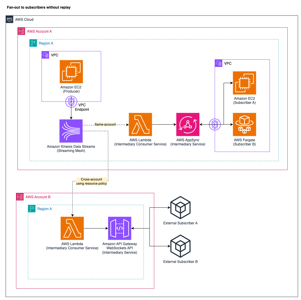
Now that you understand the overall process flow, let’s analyze the following architecture using AWS services step by step.

The first part of the preceding figure shows the data ingestion process:

  1. A user authenticates with Amazon Cognito.
  2. The user connects to the Streamlit frontend and configures the following parameters: query terms, API bearer token, and frequency to retrieve tweets.
  3. Managed Service for Apache Flink is used to consume and process the tweets in real time and stores in Apache Flink’s state the parameters for making the API requests received from the frontend application.
  4. The streaming application uses Apache Flink’s async I/O to invoke the Amazon Titan Embeddings model through the Amazon Bedrock API.
  5. Amazon Bedrock returns a vector embedding for each tweet.
  6. The Apache Flink application then writes the vector embedding with the original text of the tweet into an OpenSearch Service k-NN index.

The remainder of the architecture diagram shows the insights retrieval process:

  1. A user sends a query through the Streamlit frontend application.
  2. An AWS Lambda function is invoked by Amazon API Gateway, passing the user query as input.
  3. The Lambda function uses LangChain to orchestrate the RAG process. As a first step, the function invokes the Amazon Titan Embeddings model on Amazon Bedrock to create a vector embedding for the question.
  4. Amazon Bedrock returns the vector embedding for the question.
  5. As a second step in the RAG orchestration process, the Lambda function performs a semantic search in OpenSearch Service and retrieves the relevant documents related to the question.
  6. OpenSearch Service returns the relevant documents containing the tweet text to the Lambda function.
  7. As a last step in the LangChain orchestration process, the Lambda function augments the prompt, adding the context and using few-shot prompting. The augmented prompt, including instructions, examples, context, and query, is sent to the Anthropic Claude model through the Amazon Bedrock API.
  8. Amazon Bedrock returns the answer to the question in natural language to the Lambda function.
  9. The response is sent back to the user through API Gateway.
  10. API Gateway provides the response to the user question in the Streamlit application.

The solution is available in the GitHub repo. Follow the README file to deploy the solution.

Now that you understand the overall flow and architecture, let’s dive deeper into some of the key steps to understand how it works.

Amazon Bedrock chatbot UI

The Amazon Bedrock chatbot Streamlit application is designed to provide insights from tweets, whether they are real tweets ingested from the X API or simulated tweets or messages from the My Social Media application.

In the Streamlit application, we can provide the parameters that will be used to make the API requests to the X Developer API and pull the data from X. We developed an Apache Flink application that adjusts the API requests based on the provided parameters.

As parameters, you need to provide the following:

  • Bearer token for API authorization – This is obtained from the X Developer platform when you sign up to use the APIs.
  • Query terms to be used to filter the tweets consumed – You can use the search operators available in the X documentation.
  • Frequency of the request – The X basic API only allows you to make a request every 15 seconds. If a lower interval is set, the application won’t pull data.

The parameters are sent to Kinesis Data Streams through API Gateway and are consumed by the Apache Flink application.

My Social Media UI

The My Social Media application is a Streamlit application that serves as an additional UI. Through this application, users can compose and send messages, simulating the experience of posting on a social media site. These messages are then ingested into an AWS data pipeline consisting of API Gateway, Kinesis Data Streams, and an Apache Flink application. The Apache Flink application processes the incoming messages, invokes an Amazon Bedrock embedding model, and stores the data in an OpenSearch Service cluster.

To accommodate both real X data and simulated data from the My Social Media application, we’ve set up separate indexes within the OpenSearch Service cluster. This separation allows users to choose which data source they want to analyze or query. The Streamlit application features a sidebar option called Use X Index that acts as a toggle. When this option is enabled, the application queries and analyzes data from the index containing real tweets ingested from the X API. If the option is disabled, the application queries and displays data from the index containing messages sent through the My Social Media application.

Apache Flink is used because of its ability to scale with the increasing volume of tweets. The Apache Flink application is responsible for performing data ingestion as explained previously. Let’s dive into the details of the flow.

Consume data from X

We use Apache Flink to process the API parameters sent from the Streamlit UI. We store the parameters in Apache Flink’s state, which allows us to modify and update the parameters without having to restart the application. We use the ProcessFunction to use Apache Flink’s internal timers to schedule the frequency of requests to fetch tweets. In this post, we use X’s Recent search API, which allows us to access filtered public tweets posted over the last 7 days. The API response is paginated and returns a maximum of 100 tweets on each request in reverse chronological order. If there are more tweets to be consumed, the response of the previous request will return a token, which needs to be used in the next API call. After we receive the tweets from the API, we apply the following transformations:

  • Filter out the empty tweets (tweets without any text).
  • Partition the set of tweets by author ID. This helps distribute the processing to multiple subtasks in Apache Flink.
  • Apply a deduplication logic to only process tweets that haven’t been processed. For this, we store the already processed tweet ID in Apache Flink’s state and match and filter out the tweets that have already been processed. We store the tweets’ ID grouped by author ID, which can cause the state size of the application to increase. Because the API only provides tweets from the last 7 days when invoked, we have introduced a time-to-live (TTL) of 7 days so we don’t grow the application’s state indefinitely. You can modify this based on your requirements.
  • Convert tweets into JSON objects for a later Amazon Bedrock API invocation.

Create vector embeddings

The vector embeddings are created by invoking the Amazon Titan Embeddings model through the Amazon Bedrock API. Asynchronous invocations of external APIs are important performance considerations when building a stream processing architecture. Synchronous calls increase latency, reduce throughput, and can be a bottleneck for overall processing.

To invoke the Amazon Bedrock API, you will use the Amazon Bedrock Runtime dependency in Java, which provides an asynchronous client that allows us invoke Amazon Bedrock models asynchronously through the BedrockRuntimeAsyncClient. This is invoked to create the embeddings. For this we use Apache Flink’s async I/O to make asynchronous requests to external APIs. Apache Flink’s async I/O is a library within Apache Flink that allows you to write asynchronous, non-blocking operators for stream processing applications, enabling better utilization of resources and higher throughput. We provide the asynchronous function to be called, the timeout duration that determines how long an asynchronous operation can take before it’s considered failed, and the maximum number of requests that should be in progress at any point in time. Limiting the number of concurrent requests makes sure that the operator won’t accumulate an ever-growing backlog of pending requests. However, this can cause backpressure after the capacity is exhausted. Because we use the timestamp of creation when we ingest into OpenSearch Service and so order won’t affect our results, we can use Apache Flink’s async I/O unordered function, allowing us to have better throughput and performance. See the following code:

DataStream<JSONObject> resultStream = AsyncDataStream

.unorderedWait(inputJSON, new BedRockEmbeddingModelAsyncTweetFunction(), 15000, TimeUnit.MILLISECONDS, 1000)
.uid("tweet-async-function");

Let’s have a closer look into the Apache Flink async I/O function. The following is within the CompletableFuture Java class:

  1. First, we create the Amazon Bedrock Runtime async client:
BedrockRuntimeAsyncClient runtime = BedrockRuntimeAsyncClient.builder()
.region(Region.of(region))  // Use the specified AWS region 
.build();
  1. We then extract the tweet for the event and build the payload that we will send to Amazon Bedrock:
String stringBody = jsonObject.getString("tweet");

ArrayList<String> stringList = new ArrayList<>();


stringList.add(stringBody);


JSONObject jsonBody = new JSONObject()
.put("inputText", stringBody);


SdkBytes body = SdkBytes.fromUtf8String(jsonBody.toString());
  1. After we have the payload, we can call the InvokeModel API and invoke Amazon Titan to create the vector embeddings for the tweets:
InvokeModelRequest request = InvokeModelRequest.builder()
        
.modelId("amazon.titan-embed-text-v1")
        
.contentType("application/json")
        
.accept("*/*")
        
.body(body)
        
.build();

CompletableFuture<InvokeModelResponse> futureResponse = runtime.invokeModel(request);
  1. After receiving the vector, we append the following fields to the output JSONObject:
    1. Cleaned tweet
    2. Tweet creation timestamp
    3. Number of likes of the tweet
    4. Number of retweets
    5. Number of views from the tweet (impressions)
    6. Tweet ID
// Extract and process the response when it is available
JSONObject response = new JSONObject(
        futureResponse.join().body().asString(StandardCharsets.UTF_8)
);

// Add additional fields related to tweet data to the response
response.put("tweet", jsonObject.get("tweet"));
response.put("@timestamp", jsonObject.get("created_at"));
response.put("likes", jsonObject.get("likes"));
response.put("retweet_count", jsonObject.get("retweet_count"));
response.put("impression_count", jsonObject.get("impression_count"));
response.put("_id", jsonObject.get("_id"));

return response;

This will return the embeddings, original text, additional fields, and the number of tokens used for the embedding. In our connector, we are only consuming messages in English, as well as ignoring messages that are retweets from other tweets.

The same processing steps are replicated for messages coming from the My Social Media application (manually ingested).

Store vector embeddings in OpenSearch Service

We use OpenSearch Service as a vector database for semantic search. Before we can write the data into OpenSearch Service, we need to create an index that supports semantic search. We are using the k-NN plugin. The vector database index mapping should have the following properties for storing vectors for similarity search:

"embeddings": {
        "type": "knn_vector",
        "dimension": 1536,
        "method": {
          "name": "hnsw",
          "space_type": "l2",
          "engine": "nmslib",
          "parameters": {
            "ef_construction": 128,
            "m": 24
          }
        }
      }

The key parameters are as follows:

  • type – This specifies that the field will hold vector data for a k-NN similarity search. The value should be knn_vector.
  • dimension – The number of dimensions for each vector. This must match the model dimension. In this case we use 1,536 dimensions, the same as the Amazon Titan Text Embeddings v1 model.
  • method – Defines the algorithm and parameters for indexing and searching the vectors:
    • name – The identifier for the nearest neighbor method. We use hierarchical navigable small worlds (HNSW)—a hierarchical proximity graph approach—to run a approximate k-NN (A-NN) search because standard k-NN is not a scalable approach.
    • space_type – The vector space used to calculate the distance between vectors. It supports multiple space type. The default value is 12.
    • engine – The approximate k-NN library to use for indexing and search. The available libraries are faiss, nmslib, and Lucene.
    • ef_construction – The size of the dynamic list used during k-NN graph creation. Higher values result in a more accurate graph but slower indexing speed.
    • m – The number of bidirectional links that the plugin creates for each new element. Increasing and decreasing this value can have a large impact on memory consumption. Keep this value between 2–100.

Standard k-NN search methods compute similarity using a brute-force approach that measures the nearest distance between a query and a number of points, which produces exact results. This works well for most applications. However, in the case of extremely large datasets with high dimensionality, this creates a scaling problem that reduces the efficiency of the search. The approximate k-NN search methods used by OpenSearch Service use approximate nearest neighbor (ANN) algorithms from the nmslib, faiss, and Lucene libraries to power k-NN search. These search methods employ ANN to improve search latency for large datasets. Of the three search methods the k-NN plugin provides, this method offers the best search scalability for large datasets. This approach is the preferred method when a dataset reaches hundreds of thousands of vectors. For more information about the different methods and their trade-offs, refer to Comprehensive Guide To Approximate Nearest Neighbors Algorithms.

To use the k-NN plugin’s approximate search functionality, we must first create a k-NN index with index.knn set to true:

    "settings" : {
      "index" : {
        "knn": true,
        "number_of_shards" : "5",
        "number_of_replicas" : "1"
      }
    }

After we have our indexes created, we can sink the data from our Apache Flink application into OpenSearch.

RetrievalQA using Lambda and LangChain implementation

For this part, we take an input question from the user and invoke a Lambda function. The Lambda function retrieves relevant tweets from OpenSearch Service as context and generates an answer using the LangChain RAG chain RetrievalQA. LangChain is a framework for developing applications powered by language models.

First, some setup. We instantiate the bedrock-runtime client that will allow the Lambda function to invoke the models:

bedrock_runtime = boto3.client("bedrock-runtime", "us-east-1")

embeddings = BedrockEmbeddings(model_id="amazon.titan-embed-text-v1", client=bedrock_runtime)

The BedrockEmbeddings class uses the Amazon Bedrock API to generate embeddings for the user’s input question. It strips new line characters from the text. Notice that we need to pass as an argument the instantiation of the bedrock_runtime client and the model ID for the Amazon Titan Text Embeddings v1 model.

Next, we instantiate the client for the OpenSearchVectorSeach LangChain class that will allow the Lambda function to connect to the OpenSearch Service domain and perform the semantic search against the previously indexed X embeddings. For the embedding function, we’re passing the embeddings model that we defined previously. This will be used during the LangChain orchestration process:

os_client = OpenSearchVectorSearch(
        index_name=aos_index,
        embedding_function=embeddings,
        http_auth=(os.environ['aosUser'], os.environ['aosPassword']),
        opensearch_url=os.environ['aosDomain'],
        timeout=300,
        use_ssl=True,
        verify_certs=True,
        connection_class=RequestsHttpConnection,
        )

We need to define the LLM model from Amazon Bedrock to use for text generation. The temperature is set to 0 to reduce hallucinations:

model_kwargs={"temperature": 0, "max_tokens": 4096}

llm = BedrockChat(
    model_id="anthropic.claude-3-haiku-20240307-v1:0",
    client=bedrock_runtime,
    model_kwargs=model_kwargs
)

Next, in our Lambda function, we create the prompt to instruct the model on the specific task of analyzing hundreds of tweets in the context. To normalize the output, we use a prompt engineering technique called few-shot prompting. Few-shot prompting allows language models to learn and generate responses based on a small number of examples or demonstrations provided in the prompt itself. In this approach, instead of training the model on a large dataset, we provide a few examples of the desired task or output within the prompt. These examples serve as a guide or conditioning for the model, enabling it to understand the context and the desired format or pattern of the response. When presented with a new input after the examples, the model can then generate an appropriate response by following the patterns and context established by the few-shot demonstrations in the prompt.

As part of the prompt, we then provide examples of questions and answers, so the chatbot can follow the same pattern when used (see the Lambda function to view the complete prompt):

template = """As a helpful agent that is an expert analysing tweets, please answer the question using only the provided tweets from the context in <context></context> tags. If you don't see valuable information on the tweets provided in the context in <context></context> tags, say you don't have enough tweets related to the question. Cite the relevant context you used to build your answer. Print in a bullet point list the top most influential tweets from the context at the end of the response.
    
    Find below some examples:
    <example1>
    question: 
    What are the main challenges or concerns mentioned in tweets about using Bedrock as a generative AI service on AWS, and how can they be addressed?
    
    answer:
    Based on the tweets provided in the context, the main challenges or concerns mentioned about using Bedrock as a generative AI service on AWS are:

1.	...
2.	...
3.	...
4.	...
...
    
    To address these concerns:

1.	...
2.	...
3.	...
4.	...
...

    Top tweets from context:

    [1] ...
    [2] ...
    [3] ...
    [4] ...

    </example1>
    
    <example2>
    ...
    </example2>
    
    Human: 
    
    question: {question}
    
    <context>
    {context}
    </context>
    
    Assistant:"""

    prompt = PromptTemplate(input_variables=["context","question"], template=template)

We then create the RetrievalQA LangChain chain using the prompt template, Anthropic Claude on Amazon Bedrock, and the OpenSearch Service retriever configured previously. The RetrievalQA LangChain chain will orchestrate the following RAG steps:

  • Invoke the text embedding model to create a vector for the user’s question
  • Perform a semantic search on OpenSearch Service using the vector to retrieve the relevant tweets to the user’s question (k=200)
  • Invoke the LLM model using the augmented prompt containing the prompt template, context (stuffed retrieved tweets) and question
chain = RetrievalQA.from_chain_type(
    llm=llm,
    verbose=True,
    chain_type="stuff",
    retriever=os_client.as_retriever(
        search_type="similarity",
        search_kwargs={
            "k": 200, 
            "space_type": "l2", 
            "vector_field": "embeddings", 
            "text_field": text_field
        }
    ),
    chain_type_kwargs = {"prompt": prompt}
)

Finally, we run the chain:

answer = chain.invoke({"query": message})

The response from the LLM is sent back to the user application. As shown in the following screenshot:

Considerations

You can extend the solution provided in this post. When you do, consider the following suggestions:

  • Configure index retention and rollover in OpenSearch Service to manage index lifecycle and data retention effectively
  • Incorporate chat history into the chatbot to provide richer context and improve the relevance of LLM responses
  • Add filters and hybrid search with the possibility to modify the weight given to the keyword and semantic search to enhance search on RAG
  • Modify the TTL for Apache Flink’s state to match your requirements (the solution in this post uses 7 days)
  • Enable logging to API Gateway and in the Streamlit application.

Summary

This post demonstrates how to combine real-time analytics with generative AI capabilities to analyze tweets related to a brand, product, or topic of interest. It uses Amazon Managed Service for Apache Flink to process tweets from the X API, create vector embeddings using the Amazon Titan Embeddings model on Amazon Bedrock, and store the embeddings in an OpenSearch Service index configured for vector similarity search—all these steps happen in real time.

The post also explains how users can input queries through a Streamlit frontend application, which invokes a Lambda function. This Lambda function retrieves relevant tweets from OpenSearch Service by performing semantic search on the stored embeddings using the LangChain RetrievalQA chain. As a result, it generates insightful answers using the Anthropic Claude LLM on Amazon Bedrock.

The solution enables identifying trends, conducting sentiment analysis, detecting nuances, addressing concerns, guiding product development, and creating targeted customer segments based on real-time X data.

To get started with generative AI, visit Generative AI on AWS for information about industry use cases, tools to build and scale generative AI applications, as well as the post Exploring real-time streaming for generative AI Applications for other use cases for streaming with generative AI.


About the Authors

Francisco Morillo is a Streaming Solutions Architect at AWS, specializing in real-time analytics architectures. With over five years in the streaming data space, Francisco has worked as a data analyst for startups and as a big data engineer for consultancies, building streaming data pipelines. He has deep expertise in Amazon Managed Streaming for Apache Kafka (Amazon MSK) and Amazon Managed Service for Apache Flink. Francisco collaborates closely with AWS customers to build scalable streaming data solutions and advanced streaming data lakes, ensuring seamless data processing and real-time insights.

Sergio Garcés Vitale is a Senior Solutions Architect at AWS, passionate about generative AI. With over 10 years of experience in the telecommunications industry, where he helped build data and observability platforms, Sergio now focuses on guiding Retail and CPG customers in their cloud adoption, as well as customers across all industries and sizes in implementing Artificial Intelligence use cases.

Subham Rakshit is a Streaming Specialist Solutions Architect for Analytics at AWS based in the UK. He works with customers to design and build search and streaming data platforms that help them achieve their business objective. Outside of work, he enjoys spending time solving jigsaw puzzles with his daughter.

Optimize write throughput for Amazon Kinesis Data Streams

Post Syndicated from Buddhike de Silva original https://aws.amazon.com/blogs/big-data/optimize-write-throughput-for-amazon-kinesis-data-streams/

Amazon Kinesis Data Streams is used by many customers to capture, process, and store data streams at any scale. This level of unparalleled scale is enabled by dividing each data stream into multiple shards. Each shard in a stream has a 1 Mbps or 1,000 records per second write throughput limit. Whether your data streaming application is collecting clickstream data from a web application or recording telemetry data from billions of Internet of Things (IoT) devices, streaming applications are highly susceptible to a varying amount of data ingestion. Sometimes such a large and unexpected volume of data could be the thing we least expect. For instance, consider application logic with a retry mechanism when writing records to a Kinesis data stream. In case of a network failure, it’s common to buffer data locally and write them when connectivity is restored. Depending on the rate that data is buffered and the duration of connectivity issue, the local buffer can accumulate enough data that could saturate the available write throughput quota of a Kinesis data stream.

When an application attempts to write more data than what is allowed, it will receive write throughput exceeded errors. In some instances, not being able to address these errors in a timely manner can result in data loss, unhappy customers, and other undesirable outcomes. In this post, we explore the typical reasons behind write throughput exceeded errors, along with methods to identify them. We then guide you on swift responses to these events and provide several solutions for mitigation. Lastly, we delve into how on-demand capacity mode can be valuable in addressing these errors.

Why do we get write throughput exceeded errors?

Write throughput exceeded errors are generally caused by three different scenarios:

  • The simplest is the case where the producer application is generating more data than the throughput available in the Kinesis data stream (the sum of all shards).
  • Next, we have the case where data distribution is not even across all shards, known as hot shard issue.
  • Write throughout errors can also be caused by an application choosing a partition key to write records at a rate exceeding the throughput offered by a single shard. This situation is somewhat similar to hot shard issue, but as we see later in this post, unlike a hot shard issue, you can’t solve this problem by adding more shards to the data stream. This behavior is commonly known as a hot key issue.

Before we discuss how to diagnose these issues, let’s look at how Kinesis data streams organize data and its relationship to write throughput exceeded errors.

A Kinesis data stream has one or more shards to store data. Each shard is assigned a key range in 128-bit integer space. If you view the details of a data stream using the describe-stream operation in the AWS Command Line Interface (AWS CLI), you can actually see this key range assignment:

$ aws kinesis describe-stream --stream-name my-data-stream
"StreamDescription": {
  "Shards": [
    {
      "ShardId": "shardId-000000000000",
      "HashKeyRange": {
        "StartingHashKey": "0",
        "EndingHashKey": 
        "85070591730234615865843651857942052863"
       }
    },
    {
       "ShardId": "shardId-000000000001",
       "HashKeyRange": {
       "StartingHashKey": 
          "85070591730234615865843651857942052864",
       "EndingHashKey": 
         "170141183460469231731687303715884105727"
       }
    }
  ]
}

When a producer application invokes the PutRecord or PutRecords API, the service calculates a MD5 hash for the PartitionKey specified in the record. The resulting hash is used to determine which shard to store that record. You can take more control over this process by setting the ExplicitHashKey property in the PutRecord request to a hash key that falls within a specific shard’s key range. For instance, setting ExplicitHashKey to 0 will guarantee that record is written to shard ID shardId-0 in the stream described in the preceding code snippet.

How partition keys are distributed across available shards plays a vital role in maximizing the available throughput in a Kinesis data stream. When the partition key being used is repeated frequently in a way that some keys are more frequent than the others, shards storing those records will be utilized more. We also get the same net effect if we use ExplicitHashKey and our logic for choosing the hash key is biased towards a subset of shards.

Imagine you have a fleet of web servers logging performance metrics for each web request served into a Kinesis data stream with two shards and you used a request URL as the partition key. Each time a request is served, the application makes a call to the PutRecord API carrying a 10-bytes record. Let’s say that you have a total of 10 URLs and each receives 10 requests per second. Under these circumstances, total throughput required for the workload is 1,000 bytes per second and 100 requests per second. If we assume perfect distribution of 10 URLs across the two shards, each shard will receive 500 bytes per second and 50 requests per second.

Now imagine one of these URLs went viral and it started receiving 1,000 requests per second. Although the situation is positive from a business point of view, you’re now on the brink of making users unhappy. After the page gained popularity, you’re now counting 1,040 requests per second for the shard storing the popular URL (1000 + 10 * 4). At this point, you’ll receive write throughput exceeded errors from that shard. You’re throttled based on the requests per second quota because even with increased requests, you’re still generating approximately 11 KB of data.

You can solve this problem either by using a UUID for each request as the partition key so that you share the total load across both shards, or by adding more shards to the Kinesis data stream. The method you choose depends on how you want to consume data. Changing the partition key to a UUID would be problematic if you want performance metrics from a given URL to be always processed by the same consumer instance or if you want to maintain the order of records on a per-URL basis.

Knowing the exact cause of write throughout exceeded errors is an important step in remediating them. In the next sections, we discuss how to identify the root cause and remediate this problem.

Identifying the cause of write throughput exceeded errors

The first step in solving a problem is that knowing that it exists. You can use the WriteProvisionedThrougputExceeded metric in Amazon CloudWatch in this case. You can correlate the spikes in the WriteProvisionedThrougputExceeded metric to the IncomingBytes and IncomingRecords metrics to identify whether an application is getting throttled due to the size of data or the number of records written.

Let’s look at a few tests we performed in a stream with two shards to illustrate various scenarios. In this instance, with two shards in our stream, total throughput available to our producer application is either 2 Mbps or 2,000 records per second.

In the first test, we ran a producer to write batches of 30 records, each being 100 KB, using the PutRecords API. As you can see in the graph on the left of the following figure, our WriteProvisionedThroughputExceedded errors count went up. The graph on the right shows that we are reaching the 2 Mbps limit, but our incoming records rate is much lower than the 2,000 records per second limit (Kinesis metrics are published at 1-minute intervals, hence 125.8 and 120,000 as upper limits).Record size based throttling example

The following figures show how the same three metrics changed when we changed the producer to write batches of 500 records, each being 50 bytes, in the second test. This time, we exceeded the 2,000 records per second throughput limit, but our incoming bytes rate is well under the limit.

Record count based throttling

Now that we know that problem exists, we should look for clues to see if we’re exceeding the overall throughput available in the stream or if we’re having a hot shard issue due to an imbalanced partition key distribution as discussed earlier. One approach to this is to use enhanced shard-level metrics. Prior to our tests, we enabled enhanced shard-level metrics, and we can see in the following figure that both shards equally reached their quota in our first test.

Enhanced shard level metrics

We have seen Kinesis data streams containing thousands of shards harnessing the power of infinite scale in Kinesis data streams. However, plotting enhanced shard-level metrics on a such large stream may not provide an easy to way to find out which shards are over-utilized. In that instance, it’s better to use CloudWatch Metrics Insights to run queries to view top-n items, as shown in the following code (adjust the LIMIT 5 clause accordingly):

-- Show top 5 shards with highest incoming bytes
SELECT
SUM(IncomingBytes)
FROM "AWS/Kinesis"
GROUP BY ShardId, StreamName
ORDER BY MAX() DESC
LIMIT 5

-- Show top 5 shards with highest incoming records
SELECT
SUM(IncomingRecords)
FROM "AWS/Kinesis"
GROUP BY ShardId, StreamName
ORDER BY MAX() DESC
LIMIT 5

Enhanced shard-level metrics are not enabled by default. If you didn’t enable them and you want to perform root cause analysis after an incident, this option isn’t very helpful. In addition, you can only query the most recent 3 hours of data. Enhanced shard-level metrics also incur additional costs for CloudWatch metrics and it may be cost prohibitive to have it always on in data streams with a lot of shards.

One interesting scenario is when the workload is bursty, which can make the resulting CloudWatch metrics graphs rather baffling. This is because Kinesis publishes CloudWatch metric data aggregated at 1-minute intervals. Consequently, although you can see write throughput exceeded errors, your incoming bytes/records graphs may be still within the limits. To illustrate this scenario, we changed our test to create a burst of writes exceeding the limits and then sleep for a few seconds. Then we repeated this cycle for several minutes to yield the graphs in the following figure, which show write throughput exceeded errors on the left, but the IncomingBytes and IncomingRecords graphs on the right seem fine.

Effect of one data aggregated at 1-minute intervals

To enhance the process of identifying write throughput exceeded errors, we developed a CLI tool called Kinesis Hot Shard Advisor (KHS). With KHS, you can view shard utilization when shard-level metrics are not enabled. This is particularly useful for investigating an issue retrospectively. It can also show most frequently written keys to a particular shard. KHS reports shard utilization by reading records and aggregating them per second intervals based on the ApproximateArrivalTimestamp in the record. Because of this, you can also understand shard utilization drivers during bursty write workloads.

By running the following command, we can get KHS to inspect the data that arrived in 1 minute during our first test and generate a report:

khs -stream my-data-stream -from "2023-06-22 17:35:00" -to "2023-06-22 17:36:00"

For the given time window, the summary section in the generated report shows the maximum bytes per second rate observed, total bytes ingested, maximum records per second observed, and the total number of records ingested for each shard.

KHS report summary

Choosing a shard ID in the first column will display a graph of incoming bytes and records for that shard. This is similar to the graph you get in CloudWatch metrics, except the KHS graph reports on a per-second basis. For instance, in the following figure, we can see how the producer was going through a series of bursty writes followed by a throttling event during our test case.

KHS shard level metrics display

Running the same command with the -aggregate-key option enables partition key distribution analysis. It generates an additional graph for each shard showing the key distribution, as shown in the following figure. For our test scenario, we can only see each key being used one time because we used a new UUID for each record.

KHS key distribution graph

Because KHS reports based on data stored in streams, it creates an enhanced fan-out consumer at startup to prevent using the read throughput quota available for other consumers. When the analysis is complete, it deletes that enhanced fan-out consumer.

Due its nature of reading data streams, KHS can transfer a lot of data during analysis. For instance, assume you have a stream with 100 shards. If all of them are fully utilized during a minute window specified using -from and -to arguments, the host running KHS will receive at least 1 MB * 100 * 60 = 6000 MB = approximately 6 GB data. To avoid this kind of excessive data transfer and speed up the analysis process, we recommend first using the WriteProvisionedThroughoutExceeded CloudWatch metric to identify a time period when you experienced throttling and use a small window (such as 10 seconds) with KHS. You can also run KHS in an Amazon Elastic Compute Cloud (Amazon EC2) instance in the same AWS Region as your Kinesis data stream to minimize network latency during reads.

KHS is designed to run in a single machine to diagnose large-scale workloads. Using a naive in-memory-based counting algorithm (such as a hash map storing the partition key and count) for partition key distribution analysis could easily exhaust the available memory in the host system. Therefore, we use a probabilistic data structure called count-min-sketch to estimate the number of times a key has been used. As a result, the number you see in the report should be taken as an approximate value rather than an absolute value. After all, with this report, we just want to find out if there’s an imbalance in the keys written to a shard.

Now that we understand what causes hot shards and how to identify them, let’s look at how to deal with this in producer applications and remediation steps.

Remediation steps

Having producers retry writes is a step towards making our producers resilient to write throughput exceeded errors. Consider our earlier sample application logging performance metrics data for each web request served by a fleet of web servers. When implementing this retry mechanism, you should remember that records that are not written to the Kinesis stream are going to be in host system’s memory. The first issue with this is, if the host crashes before the records could be written, you’ll experience data loss. Scenarios such as tracking web request performance data might be more forgiving for this type of data loss than scenarios like financial transactions. You should evaluate durability guarantees required for your application and employ techniques to achieve them.

The second issue is that records waiting to be written to the Kinesis data stream are going to consume the host system’s memory. When you start getting throttled and have some retry logic in place, you should notice that your memory utilization is going up. A retry mechanism should have a way to avoid exhausting the host system’s memory.

With the appropriate retry logic in place, if you receive write throughput exceeded errors, you can use the methods we discussed earlier to identify the cause. After you identify the root cause, you can choose the appropriate remediation step:

  • If the producer application is exceeding the overall stream’s throughput, you can add more shards to the stream to increase its write throughput capacity. When adding shards, the Kinesis data stream makes the new shards available incrementally, minimizing the time that producers experience write throughput exceeded errors. To add shards to a stream, you can use the Kinesis console, the update-shard-count operation in the AWS CLI, the UpdateShardCount API through the AWS SDK, or the ShardCount property in the AWS CloudFormation template used to create the stream.
  • If the producer application is exceeding the throughput limit of some shards (hot shard issue), pick one of the following options based on consumer requirements:
    • If locality of data is required (records with the same partition key are always processed by the same consumer) or an order based on partition key is required, use the split-shard operation in the AWS CLI or the SplitShard API in the AWS SDK to split those shards.
    • If locality or order based on the current partition key is not required, change the partition key scheme to increase its distribution.
  • If the producer application is exceeding the throughput limit of a shard due to a single partition key (hot key issue), change the partition key scheme to increase its distribution.

Kinesis Data Streams also has an on-demand capacity mode. In on-demand capacity mode, Kinesis Data Streams automatically scales streams when needed. Additionally, you can switch between on-demand and provisioned capacity modes without causing an outage. This could be particularly useful when you’re experiencing write throughput exceeded errors but require immediate reaction to keep your application available to your users. In such instances, you can switch a provisioned capacity mode data stream to an on-demand data stream and let Kinesis Data Streams handle the required scale appropriately. You can then perform root cause analysis in the background and take corrective actions. Finally, if necessary, you can change the capacity mode back to provisioned.

Conclusion

You should now have a solid understanding of the common causes of write throughput exceeded errors in Kinesis data streams, how to diagnose them, and what actions to take to appropriately deal with them. We hope that this post will help you make your Kinesis Data Streams applications more robust. If you are just starting with Kinesis Data Streams, we recommend referring to the Developer Guide.

If you have any questions or feedback, please leave them in the comments section.


About the Authors

Buddhike de Silva is a Senior Specialist Solutions Architect at Amazon Web Services. Buddhike helps customers run large scale streaming analytics workloads on AWS and make the best out of their cloud journey.

Nihar Sheth is a Senior Product Manager at Amazon Web Services. He is passionate about developing intuitive product experiences that solve complex customer problems and enable customers to achieve their business goals.

Architectural Patterns for real-time analytics using Amazon Kinesis Data Streams, Part 2: AI Applications

Post Syndicated from Raghavarao Sodabathina original https://aws.amazon.com/blogs/big-data/architectural-patterns-for-real-time-analytics-using-amazon-kinesis-data-streams-part-2-ai-applications/

Welcome back to our exciting exploration of architectural patterns for real-time analytics with Amazon Kinesis Data Streams! In this fast-paced world, Kinesis Data Streams stands out as a versatile and robust solution to tackle a wide range of use cases with real-time data, from dashboarding to powering artificial intelligence (AI) applications. In this series, we streamline the process of identifying and applying the most suitable architecture for your business requirements, and help kickstart your system development efficiently with examples.

Before we dive in, we recommend reviewing Architectural patterns for real-time analytics using Amazon Kinesis Data Streams, part 1 for the basic functionalities of Kinesis Data Streams. Part 1 also contains architectural examples for building real-time applications for time series data and event-sourcing microservices.

Now get ready as we embark on the second part of this series, where we focus on the AI applications with Kinesis Data Streams in three scenarios: real-time generative business intelligence (BI), real-time recommendation systems, and Internet of Things (IoT) data streaming and inferencing.

Real-time generative BI dashboards with Kinesis Data Streams, Amazon QuickSight, and Amazon Q

In today’s data-driven landscape, your organization likely possesses a vast amount of time-sensitive information that can be used to gain a competitive edge. The key to unlock the full potential of this real-time data lies in your ability to effectively make sense of it and transform it into actionable insights in real time. This is where real-time BI tools such as live dashboards come into play, assisting you with data aggregation, analysis, and visualization, therefore accelerating your decision-making process.

To help streamline this process and empower your team with real-time insights, Amazon has introduced Amazon Q in QuickSight. Amazon Q is a generative AI-powered assistant that you can configure to answer questions, provide summaries, generate content, and complete tasks based on your data. Amazon QuickSight is a fast, cloud-powered BI service that delivers insights.

With Amazon Q in QuickSight, you can use natural language prompts to build, discover, and share meaningful insights in seconds, creating context-aware data Q&A experiences and interactive data stories from the real-time data. For example, you can ask “Which products grew the most year-over-year?” and Amazon Q will automatically parse the questions to understand the intent, retrieve the corresponding data, and return the answer in the form of a number, chart, or table in QuickSight.

By using the architecture illustrated in the following figure, your organization can harness the power of streaming data and transform it into visually compelling and informative dashboards that provide real-time insights. With the power of natural language querying and automated insights at your fingertips, you’ll be well-equipped to make informed decisions and stay ahead in today’s competitive business landscape.

Build real-time generative business intelligence dashboards with Amazon Kinesis Data Streams, Amazon QuickSight, and Amazon Qtreaming & inferencing pipeline with AWS IoT & Amazon SageMaker

The steps in the workflow are as follows:

  1. We use Amazon DynamoDB here as an example for the primary data store. Kinesis Data Streams can ingest data in real time from data stores such as DynamoDB to capture item-level changes in your table.
  2. After capturing data to Kinesis Data Streams, you can ingest the data into analytic databases such as Amazon Redshift in near-real time. Amazon Redshift Streaming Ingestion simplifies data pipelines by letting you create materialized views directly on top of data streams. With this capability, you can use SQL (Structured Query Language) to connect to and directly ingest the data stream from Kinesis Data Streams to analyze and run complex analytical queries.
  3. After the data is in Amazon Redshift, you can create a business report using QuickSight. Connectivity between a QuickSight dashboard and Amazon Redshift enables you to deliver visualization and insights. With the power of Amazon Q in QuickSight, you can quickly build and refine the analytics and visuals with natural language inputs.

For more details on how customers have built near real-time BI dashboards using Kinesis Data Streams, refer to the following:

Real-time recommendation systems with Kinesis Data Streams and Amazon Personalize

Imagine creating a user experience so personalized and engaging that your customers feel truly valued and appreciated. By using real-time data about user behavior, you can tailor each user’s experience to their unique preferences and needs, fostering a deep connection between your brand and your audience. You can achieve this by using Kinesis Data Streams and Amazon Personalize, a fully managed machine learning (ML) service that generates product and content recommendations for your users, instead of building your own recommendation engine from scratch.

With Kinesis Data Streams, your organization can effortlessly ingest user behavior data from millions of endpoints into a centralized data stream in real time. This allows recommendation engines such as Amazon Personalize to read from the centralized data stream and generate personalized recommendations for each user on the fly. Additionally, you could use enhanced fan-out to deliver dedicated throughput to your mission-critical consumers at even lower latency, further enhancing the responsiveness of your real-time recommendation system. The following figure illustrates a typical architecture for building real-time recommendations with Amazon Personalize.

Build real-time recommendation systems with Kinesis Data Streams and Amazon Personalize

The steps are as follows:

  1. Create a dataset group, schemas, and datasets that represent your items, interactions, and user data.
  2. Select the best recipe matching your use case after importing your datasets into a dataset group using Amazon Simple Storage Service(Amazon S3), and then create a solution to train a model by creating a solution version. When your solution version is complete, you can create a campaign for your solution version.
  3. After a campaign has been created, you can integrate calls to the campaign in your application. This is where calls to the GetRecommendations or GetPersonalizedRanking APIs are made to request near-real-time recommendations from Amazon Personalize. Your website or mobile application calls a AWS Lambda function over Amazon API Gateway to receive recommendations for your business apps.
  4. An event tracker provides an endpoint that allows you to stream interactions that occur in your application back to Amazon Personalize in near-real time. You do this by using the PutEvents API. You can build an event collection pipeline using API Gateway, Kinesis Data Streams, and Lambda to receive and forward interactions to Amazon Personalize. The event tracker performs two primary functions. First, it persists all streamed interactions so they will be incorporated into future retrainings of your model. This is also how Amazon Personalize cold starts new users. When a new user visits your site, Amazon Personalize will recommend popular items. After you stream in an event or two, Amazon Personalize immediately starts adjusting recommendations.

To learn how other customers have built personalized recommendations using Kinesis Data Streams, refer to the following:

Real-time IoT data streaming and inferencing with AWS IoT Core and Amazon SageMaker

From office lights that automatically turn on as you enter the room to medical devices that monitors a patient’s health in real time, a proliferation of smart devices is making the world more automated and connected. In technical terms, IoT is the network of devices that connect with the internet and can exchange data with other devices and software systems. Many organizations increasingly rely on the real-time data from IoT devices, such as temperature sensors and medical equipment, to drive automation, analytics, and AI systems. It’s important to choose a robust streaming solution that can achieve very low latency and handle high volumes of data throughputs to power the real-time AI inferencing.

With Kinesis Data Streams, IoT data across millions of devices can simultaneously write to a centralized data stream. Alternatively, you can use AWS IoT Core to securely connect and easily manage the fleet of IoT devices, collect the IoT data, and then ingest to Kinesis Data Streams for real-time transformation, analytics, and event-driven microservices. Then, you can use integrated services such as Amazon SageMaker for real-time inference. The following diagram depicts the high-level streaming architecture with IoT sensor data.

Build real-time IoT data streaming & inferencing pipeline with AWS IoT & Amazon SageMaker

The steps are as follows:

  1. Data originates in IoT devices such as medical devices, car sensors, and industrial IoT sensors. This telemetry data is collected using AWS IoT Greengrass, an open source IoT edge runtime and cloud service that helps your devices collect and analyze data closer to where the data is generated.
  2. Event data is ingested into the cloud using edge-to-cloud interface services such as AWS IoT Core, a managed cloud platform that connects, manages, and scales devices effortlessly and securely. You can also use AWS IoT SiteWise, a managed service that helps you collect, model, analyze, and visualize data from industrial equipment at scale. Alternatively, IoT devices could send data directly to Kinesis Data Streams.
  3. AWS IoT Core can stream ingested data into Kinesis Data Streams.
  4. The ingested data gets transformed and analyzed in near real time using Amazon Managed Service for Apache Flink. Stream data can further be enriched using lookup data hosted in a data warehouse such as Amazon Redshift. Managed Service for Apache Flink can persist streamed data into Amazon Redshift after the customer’s integration and stream aggregation (for example, 1 minute or 5 minutes). The results in Amazon Redshift can be used for further downstream BI reporting services, such as QuickSight. Managed Service for Apache Flink can also write to a Lambda function, which can invoke SageMaker models. After the ML model is trained and deployed in SageMaker, inferences are invoked in a microbatch using Lambda. Inferenced data is sent to Amazon OpenSearch Service to create personalized monitoring dashboards using OpenSearch Dashboards. The transformed IoT sensor data can be stored in DynamoDB. You can use AWS AppSync to provide near real-time data queries to API services for downstream applications. These enterprise applications can be mobile apps or business applications to track and monitor the IoT sensor data in near real time.
  5. The streamed IoT data can be written to an Amazon Data Firehose delivery stream, which microbatches data into Amazon S3 for future analytics.

To learn how other customers have built IoT device monitoring solutions using Kinesis Data Streams, refer to:

Conclusion

This post demonstrated additional architectural patterns for building low-latency AI applications with Kinesis Data Streams and its integrations with other AWS services. Customers looking to build generative BI, recommendation systems, and IoT data streaming and inferencing can refer to these patterns as the starting point of designing your cloud architecture. We will continue to add new architectural patterns in the future posts of this series.

For detailed architectural patterns, refer to the following resources:

If you want to build a data vision and strategy, check out the AWS Data-Driven Everything (D2E) program.


About the Authors

Raghavarao Sodabathina is a Principal Solutions Architect at AWS, focusing on Data Analytics, AI/ML, and cloud security. He engages with customers to create innovative solutions that address customer business problems and to accelerate the adoption of AWS services. In his spare time, Raghavarao enjoys spending time with his family, reading books, and watching movies.

Hang Zuo is a Senior Product Manager on the Amazon Kinesis Data Streams team at Amazon Web Services. He is passionate about developing intuitive product experiences that solve complex customer problems and enable customers to achieve their business goals.

Shwetha Radhakrishnan is a Solutions Architect for AWS with a focus in Data Analytics. She has been building solutions that drive cloud adoption and help organizations make data-driven decisions within the public sector. Outside of work, she loves dancing, spending time with friends and family, and traveling.

Brittany Ly is a Solutions Architect at AWS. She is focused on helping enterprise customers with their cloud adoption and modernization journey and has an interest in the security and analytics field. Outside of work, she loves to spend time with her dog and play pickleball.

Build Spark Structured Streaming applications with the open source connector for Amazon Kinesis Data Streams

Post Syndicated from Idan Maizlits original https://aws.amazon.com/blogs/big-data/build-spark-structured-streaming-applications-with-the-open-source-connector-for-amazon-kinesis-data-streams/

Apache Spark is a powerful big data engine used for large-scale data analytics. Its in-memory computing makes it great for iterative algorithms and interactive queries. You can use Apache Spark to process streaming data from a variety of streaming sources, including Amazon Kinesis Data Streams for use cases like clickstream analysis, fraud detection, and more. Kinesis Data Streams is a serverless streaming data service that makes it straightforward to capture, process, and store data streams at any scale.

With the new open source Amazon Kinesis Data Streams Connector for Spark Structured Streaming, you can use the newer Spark Data Sources API. It also supports enhanced fan-out for dedicated read throughput and faster stream processing. In this post, we deep dive into the internal details of the connector and show you how to use it to consume and produce records from and to Kinesis Data Streams using Amazon EMR.

Introducing the Kinesis Data Streams connector for Spark Structured Streaming

The Kinesis Data Streams connector for Spark Structured Streaming is an open source connector that supports both provisioned and On-Demand capacity modes offered by Kinesis Data Streams. The connector is built using the latest Spark Data Sources API V2, which uses Spark optimizations. Starting with Amazon EMR 7.1, the connector comes pre-packaged on Amazon EMR on Amazon EKS, Amazon EMR on Amazon EC2, and Amazon EMR Serverless, so you don’t need to build or download any packages. For using it with other Apache Spark platforms, the connector is available as a public JAR file that can be directly referred to while submitting a Spark Structured Streaming job. Additionally, you can download and build the connector from the GitHub repo.

Kinesis Data Streams supports two types of consumers: shared throughput and dedicated throughput. With shared throughput, 2 Mbps of read throughput per shard is shared across consumers. With dedicated throughput, also known as enhanced fan-out, 2 Mbps of read throughput per shard is dedicated to each consumer. This new connector supports both consumer types out of the box without any additional coding, providing you the flexibility to consume records from your streams based on your requirements. By default, this connector uses a shared throughput consumer, but you can configure it to use enhanced fan-out in the configuration properties.

You can also use the connector as a sink connector to produce records to a Kinesis data stream. The configuration parameters for using the connector as a source and sink differ—for more information, see Kinesis Source Configuration. The connector also supports multiple storage options, including Amazon DynamoDB, Amazon Simple Service for Storage (Amazon S3), and HDFS, to store checkpoints and provide continuity.

For scenarios where a Kinesis data stream is deployed in an AWS producer account and the Spark Structured Streaming application is in a different AWS consumer account, you can use the connector to do cross-account processing. This requires additional Identity and Access Management (IAM) trust policies to allow the Spark Structured Streaming application in the consumer account to assume the role in the producer account.

You should also consider reviewing the security configuration with your security teams based on your data security requirements.

How the connector works

Consuming records from Kinesis Data Streams using the connector involves multiple steps. The following architecture diagram shows the internal details of how the connector works. A Spark Structured Streaming application consumes records from a Kinesis data stream source and produces records to another Kinesis data stream.

A Kinesis data stream is composed of set of shards. A shard is a uniquely identified sequence of data records in a stream and provides a fixed unit of capacity. The total capacity of the stream is the sum of the capacity of all of its shards.

A Spark application consists of a driver and a set of executor processes. The Spark driver acts as a coordinator, and the tasks running in executors are responsible for producing and consuming records to and from shards.

The solution workflow includes the following steps:

  1. Internally, by default, Structured Streaming queries are processed using a micro-batch processing engine, which processes data streams as a series of small batch jobs. At the beginning of a micro-batch run, the driver uses the Kinesis Data Streams ListShard API to determine the latest description of all available shards. The connector exposes a parameter (kinesis.describeShardInterval) to configure the interval between two successive ListShard API calls.
  2. The driver then determines the starting position in each shard. If the application is a new job, the starting position of each shard is determined by kinesis.startingPosition. If it’s a restart of an existing job, it’s read from last record metadata checkpoint from storage (for this post, DynamoDB) and ignores kinesis.startingPosition.
  3. Each shard is mapped to one task in an executor, which is responsible for reading data. The Spark application automatically creates an equal number of tasks based on the number of shards and distributes it across the executors.
  4. The tasks in an executor use either polling mode (shared) or push mode (enhanced fan-out) to get data records from the starting position for a shard.
  5. Spark tasks running in the executors write the processed data to the data sink. In this architecture, we use the Kinesis Data Streams sink to illustrate how the connector writes back to the stream. Executors can write to more than one Kinesis Data Streams output shard.
  6. At the end of each task, the corresponding executor process saves the metadata (checkpoint) about the last record read for each shard in the offset storage (for this post, DynamoDB). This information is used by the driver in the construction of the next micro-batch.

Solution overview

The following diagram shows an example architecture of how to use the connector to read from one Kinesis data stream and write to another.

In this architecture, we use the Amazon Kinesis Data Generator (KDG) to generate sample streaming data (random events per country) to a Kinesis Data Streams source. We start an interactive Spark Structured Streaming session and consume data from the Kinesis data stream, and then write to another Kinesis data stream.

We use Spark Structured Streaming to count events per micro-batch window. These events for each country are being consumed from Kinesis Data Streams. After the count, we can see the results.

Prerequisites

To get started, follow the instructions in the GitHub repo. You need the following prerequisites:

After you deploy the solution using the AWS CDK, you will have the following resources:

  • An EMR cluster with the Kinesis Spark connector installed
  • A Kinesis Data Streams source
  • A Kinesis Data Streams sink

Create your Spark Structured Streaming application

After the deployment is complete, you can access the EMR primary node to start a Spark application and write your Spark Structured Streaming logic.

As we mentioned earlier, you use the new open source Kinesis Spark connector to consume data from Amazon EMR. You can find the connector code on the GitHub repo along with examples on how to build and set up the connector in Spark.

In this post, we use Amazon EMR 7.1, where the connector is natively available. If you’re not using Amazon EMR 7.1 and above, you can use the connector by running the following code:

cd /usr/lib/spark/jars 
sudo wget https://awslabs-code-us-east-1.s3.amazonaws.com/spark-sql-kinesis-connector/spark-streaming-sql-kinesis-connector_2.12-1.2.1.jar
sudo chmod 755 spark-streaming-sql-kinesis-connector_2.12-1.2.1.jar

Complete the following steps:

  1. On the Amazon EMR console, navigate to the emr-spark-kinesis cluster.
  2. On the Instances tab, select the primary instance and choose the Amazon Elastic Compute Cloud (Amazon EC2) instance ID.

You’re redirected to the Amazon EC2 console.

  1. On the Amazon EC2 console, select the primary instance and choose Connect.
  2. Use Session Manager, a capability of AWS Systems Manager, to connect to the instance.
  3. Because the user that is used to connect is the ssm-user, we need to switch to the Hadoop user:
    sudo su hadoop

  4. Start a Spark shell either using Scala or Python to interactively build a Spark Structured Streaming application to consume data from a Kinesis data stream.

For this post, we use Python for writing to a stream using a PySpark shell in Amazon EMR.

  1. Start the PySpark shell by entering the command pyspark.

Because you already have the connector installed in the EMR cluster, you can now create the Kinesis source.

  1. Create the Kinesis source with the following code:
    kinesis = spark.readStream.format("aws-kinesis") \
        .option("kinesis.region", "<aws-region>") \
        .option("kinesis.streamName", "kinesis-source") \
        .option("kinesis.consumerType", "GetRecords") \
        .option("kinesis.endpointUrl", "https://kinesis.<aws-region>.amazonaws.com") \
        .option("kinesis.startingposition", "LATEST") \
        .load()

For creating the Kinesis source, the following parameters are required:

  • Name of the connector – We use the connector name aws-kinesis
  • kinesis.region – The AWS Region of the Kinesis data stream you are consuming
  • kinesis.consumerType – Use GetRecords (standard consumer) or SubscribeToShard (enhanced fan-out consumer)
  • kinesis.endpointURL – The Regional Kinesis endpoint (for more details, see Service endpoints)
  • kinesis.startingposition – Choose LATEST, TRIM_HORIZON, or AT_TIMESTAMP (refer to ShardIteratorType)

For using an enhanced fan-out consumer, additional parameters are needed, such as the consumer name. The additional configuration can be found in the connector’s GitHub repo.

kinesis_efo = spark \
.readStream \
.format("aws-kinesis") \
.option("kinesis.region", "<aws-region>") \
.option("kinesis.streamName", "kinesis-source") \
.option("kinesis.consumerType", "SubscribeToShard") \
.option("kinesis.consumerName", "efo-consumer") \
.option("kinesis.endpointUrl", "https://kinesis.<aws-region>.amazonaws.com") \
.option("kinesis.startingposition", "LATEST") \
.load()

Deploy the Kinesis Data Generator

Complete the following steps to deploy the KDG and start generating data:

  1. Choose Launch Stack:
    launch stack 1

You might need to change your Region when deploying. Make sure that the KDG is launched in the same Region as where you deployed the solution.

  1. For the parameters Username and Password, enter the values of your choice. Note these values to use later when you log in to the KDG.
  2. When the template has finished deploying, go to the Outputs tab of the stack and locate the KDG URL.
  3. Log in to the KDG, using the credentials you set when launching the CloudFormation template.
  4. Specify your Region and data stream name, and use the following template to generate test data:
    {
        "id": {{random.number(100)}},
        "data": "{{random.arrayElement(
            ["Spain","Portugal","Finland","France"]
        )}}",
        "date": "{{date.now("YYYY-MM-DD hh:mm:ss")}}"
    }

  5. Return to Systems Manager to continue working with the Spark application.
  6. To be able to apply transformations based on the fields of the events, you first need to define the schema for the events:
    from pyspark.sql.types import *
    
    pythonSchema = StructType() \
     .add("id", LongType()) \
     .add("data", StringType()) \
     .add("date", TimestampType())

  7. Run the following the command to consume data from Kinesis Data Streams:
    from pyspark.sql.functions import *
    
    events= kinesis \
      .selectExpr("cast (data as STRING) jsonData") \
      .select(from_json("jsonData", pythonSchema).alias("events")) \
      .select("events.*")

  8. Use the following code for the Kinesis Spark connector sink:
    events \
        .selectExpr("CAST(id AS STRING) as partitionKey","data","date") \
        .writeStream \
        .format("aws-kinesis") \
        .option("kinesis.region", "<aws-region>") \
        .outputMode("append") \
        .option("kinesis.streamName", "kinesis-sink") \
        .option("kinesis.endpointUrl", "https://kinesis.<aws-region>.amazonaws.com") \
        .option("checkpointLocation", "/kinesisCheckpoint") \
        .start() \
        .awaitTermination()

You can view the data in the Kinesis Data Streams console.

  1. On the Kinesis Data Streams console, navigate to kinesis-sink.
  2. On the Data viewer tab, choose a shard and a starting position (for this post, we use Latest) and choose Get records.

You can see the data sent, as shown in the following screenshot. Kinesis Data Streams uses base64 encoding by default, so you might see text with unreadable characters.

Clean up

Delete the following CloudFormation stacks created during this deployment to delete all the provisioned resources:

  • EmrSparkKinesisStack
  • Kinesis-Data-Generator-Cognito-User-SparkEFO-Blog

If you created any additional resources during this deployment, delete them manually.

Conclusion

In this post, we discussed the open source Kinesis Data Streams connector for Spark Structured Streaming. It supports the newer Data Sources API V2 and Spark Structured Streaming for building streaming applications. The connector also enables high-throughput consumption from Kinesis Data Streams with enhanced fan-out by providing dedicated throughput up to 2 Mbps per shard per consumer. With this connector, you can now effortlessly build high-throughput streaming applications with Spark Structured Streaming.

The Kinesis Spark connector is open source under the Apache 2.0 license on GitHub. To get started, visit the GitHub repo.


About the Authors


Idan Maizlits is a Senior Product Manager on the Amazon Kinesis Data Streams team at Amazon Web Services. Idan loves engaging with customers to learn about their challenges with real-time data and to help them achieve their business goals. Outside of work, he enjoys spending time with his family exploring the outdoors and cooking.


Subham Rakshit is a Streaming Specialist Solutions Architect for Analytics at AWS based in the UK. He works with customers to design and build search and streaming data platforms that help them achieve their business objective. Outside of work, he enjoys spending time solving jigsaw puzzles with his daughter.

Francisco Morillo is a Streaming Solutions Architect at AWS. Francisco works with AWS customers helping them design real-time analytics architectures using AWS services, supporting Amazon MSK and AWS’s managed offering for Apache Flink.

Umesh Chaudhari is a Streaming Solutions Architect at AWS. He works with customers to design and build real-time data processing systems. He has extensive working experience in software engineering, including architecting, designing, and developing data analytics systems. Outside of work, he enjoys traveling, reading, and watching movies.

Krones real-time production line monitoring with Amazon Managed Service for Apache Flink

Post Syndicated from Florian Mair original https://aws.amazon.com/blogs/big-data/krones-real-time-production-line-monitoring-with-amazon-managed-service-for-apache-flink/

Krones provides breweries, beverage bottlers, and food producers all over the world with individual machines and complete production lines. Every day, millions of glass bottles, cans, and PET containers run through a Krones line. Production lines are complex systems with lots of possible errors that could stall the line and decrease the production yield. Krones wants to detect the failure as early as possible (sometimes even before it happens) and notify production line operators to increase reliability and output. So how to detect a failure? Krones equips their lines with sensors for data collection, which can then be evaluated against rules. Krones, as the line manufacturer, as well as the line operator have the possibility to create monitoring rules for machines. Therefore, beverage bottlers and other operators can define their own margin of error for the line. In the past, Krones used a system based on a time series database. The main challenges were that this system was hard to debug and also queries represented the current state of machines but not the state transitions.

This post shows how Krones built a streaming solution to monitor their lines, based on Amazon Kinesis and Amazon Managed Service for Apache Flink. These fully managed services reduce the complexity of building streaming applications with Apache Flink. Managed Service for Apache Flink manages the underlying Apache Flink components that provide durable application state, metrics, logs, and more, and Kinesis enables you to cost-effectively process streaming data at any scale. If you want to get started with your own Apache Flink application, check out the GitHub repository for samples using the Java, Python, or SQL APIs of Flink.

Overview of solution

Krones’s line monitoring is part of the Krones Shopfloor Guidance system. It provides support in the organization, prioritization, management, and documentation of all activities in the company. It allows them to notify an operator if the machine is stopped or materials are required, regardless where the operator is in the line. Proven condition monitoring rules are already built-in but can also be user defined via the user interface. For example, if a certain data point that is monitored violates a threshold, there can be a text message or trigger for a maintenance order on the line.

The condition monitoring and rule evaluation system is built on AWS, using AWS analytics services. The following diagram illustrates the architecture.

Architecture Diagram for Krones Production Line Monitoring

Almost every data streaming application consists of five layers: data source, stream ingestion, stream storage, stream processing, and one or more destinations. In the following sections, we dive deeper into each layer and how the line monitoring solution, built by Krones, works in detail.

Data source

The data is gathered by a service running on an edge device reading several protocols like Siemens S7 or OPC/UA. Raw data is preprocessed to create a unified JSON structure, which makes it easier to process later on in the rule engine. A sample payload converted to JSON might look like the following:

{
  "version": 1,
  "timestamp": 1234,
  "equipmentId": "84068f2f-3f39-4b9c-a995-d2a84d878689",
  "tag": "water_temperature",
  "value": 13.45,
  "quality": "Ok",
  "meta": {      
    "sequenceNumber": 123,
    "flags": ["Fst", "Lst", "Wmk", "Syn", "Ats"],
    "createdAt": 12345690,
    "sourceId": "filling_machine"
  }
}

Stream ingestion

AWS IoT Greengrass is an open source Internet of Things (IoT) edge runtime and cloud service. This allows you to act on data locally and aggregate and filter device data. AWS IoT Greengrass provides prebuilt components that can be deployed to the edge. The production line solution uses the stream manager component, which can process data and transfer it to AWS destinations such as AWS IoT Analytics, Amazon Simple Storage Service (Amazon S3), and Kinesis. The stream manager buffers and aggregates records, then sends it to a Kinesis data stream.

Stream storage

The job of the stream storage is to buffer messages in a fault tolerant way and make it available for consumption to one or more consumer applications. To achieve this on AWS, the most common technologies are Kinesis and Amazon Managed Streaming for Apache Kafka (Amazon MSK). For storing our sensor data from production lines, Krones choose Kinesis. Kinesis is a serverless streaming data service that works at any scale with low latency. Shards within a Kinesis data stream are a uniquely identified sequence of data records, where a stream is composed of one or more shards. Each shard has 2 MB/s of read capacity and 1 MB/s write capacity (with max 1,000 records/s). To avoid hitting those limits, data should be distributed among shards as evenly as possible. Every record that is sent to Kinesis has a partition key, which is used to group data into a shard. Therefore, you want to have a large number of partition keys to distribute the load evenly. The stream manager running on AWS IoT Greengrass supports random partition key assignments, which means that all records end up in a random shard and the load is distributed evenly. A disadvantage of random partition key assignments is that records aren’t stored in order in Kinesis. We explain how to solve this in the next section, where we talk about watermarks.

Watermarks

A watermark is a mechanism used to track and measure the progress of event time in a data stream. The event time is the timestamp from when the event was created at the source. The watermark indicates the timely progress of the stream processing application, so all events with an earlier or equal timestamp are considered as processed. This information is essential for Flink to advance event time and trigger relevant computations, such as window evaluations. The allowed lag between event time and watermark can be configured to determine how long to wait for late data before considering a window complete and advancing the watermark.

Krones has systems all around the globe, and needed to handle late arrivals due to connection losses or other network constraints. They started out by monitoring late arrivals and setting the default Flink late handling to the maximum value they saw in this metric. They experienced issues with time synchronization from the edge devices, which lead them to a more sophisticated way of watermarking. They built a global watermark for all the senders and used the lowest value as the watermark. The timestamps are stored in a HashMap for all incoming events. When the watermarks are emitted periodically, the smallest value of this HashMap is used. To avoid stalling of watermarks by missing data, they configured an idleTimeOut parameter, which ignores timestamps that are older than a certain threshold. This increases latency but gives strong data consistency.

public class BucketWatermarkGenerator implements WatermarkGenerator<DataPointEvent> {
private HashMap <String, WatermarkAndTimestamp> lastTimestamps;
private Long idleTimeOut;
private long maxOutOfOrderness;
}

Stream processing

After the data is collected from sensors and ingested into Kinesis, it needs to be evaluated by a rule engine. A rule in this system represents the state of a single metric (such as temperature) or a collection of metrics. To interpret a metric, more than one data point is used, which is a stateful calculation. In this section, we dive deeper into the keyed state and broadcast state in Apache Flink and how they’re used to build the Krones rule engine.

Control stream and broadcast state pattern

In Apache Flink, state refers to the ability of the system to store and manage information persistently across time and operations, enabling the processing of streaming data with support for stateful computations.

The broadcast state pattern allows the distribution of a state to all parallel instances of an operator. Therefore, all operators have the same state and data can be processed using this same state. This read-only data can be ingested by using a control stream. A control stream is a regular data stream, but usually with a much lower data rate. This pattern allows you to dynamically update the state on all operators, enabling the user to change the state and behavior of the application without the need for a redeploy. More precisely, the distribution of the state is done by the use of a control stream. By adding a new record into the control stream, all operators receive this update and are using the new state for the processing of new messages.

This allows users of Krones application to ingest new rules into the Flink application without restarting it. This avoids downtime and gives a great user experience as changes happen in real time. A rule covers a scenario in order to detect a process deviation. Sometimes, the machine data is not as easy to interpret as it might look at first glance. If a temperature sensor is sending high values, this might indicate an error, but also be the effect of an ongoing maintenance procedure. It’s important to put metrics in context and filter some values. This is achieved by a concept called grouping.

Grouping of metrics

The grouping of data and metrics allows you to define the relevance of incoming data and produce accurate results. Let’s walk through the example in the following figure.

Grouping of metrics

In Step 1, we define two condition groups. Group 1 collects the machine state and which product is going through the line. Group 2 uses the value of the temperature and pressure sensors. A condition group can have different states depending on the values it receives. In this example, group 1 receives data that the machine is running, and the one-liter bottle is selected as the product; this gives this group the state ACTIVE. Group 2 has metrics for temperature and pressure; both metrics are above their thresholds for more than 5 minutes. This results in group 2 being in a WARNING state. This means group 1 reports that everything is fine and group 2 does not. In Step 2, weights are added to the groups. This is needed in some situations, because groups might report conflicting information. In this scenario, group 1 reports ACTIVE and group 2 reports WARNING, so it’s not clear to the system what the state of the line is. After adding the weights, the states can be ranked, as shown in step 3. Lastly, the highest ranked state is chosen as the winning one, as shown in Step 4.

After the rules are evaluated and the final machine state is defined, the results will be further processed. The action taken depends on the rule configuration; this can be a notification to the line operator to restock materials, do some maintenance, or just a visual update on the dashboard. This part of the system, which evaluates metrics and rules and takes actions based on the results, is referred to as a rule engine.

Scaling the rule engine

By letting users build their own rules, the rule engine can have a high number of rules that it needs to evaluate, and some rules might use the same sensor data as other rules. Flink is a distributed system that scales very well horizontally. To distribute a data stream to several tasks, you can use the keyBy() method. This allows you to partition a data stream in a logical way and send parts of the data to different task managers. This is often done by choosing an arbitrary key so you get an evenly distributed load. In this case, Krones added a ruleId to the data point and used it as a key. Otherwise, data points that are needed are processed by another task. The keyed data stream can be used across all rules just like a regular variable.

Destinations

When a rule changes its state, the information is sent to a Kinesis stream and then via Amazon EventBridge to consumers. One of the consumers creates a notification from the event that is transmitted to the production line and alerts the personnel to act. To be able to analyze the rule state changes, another service writes the data to an Amazon DynamoDB table for fast access and a TTL is in place to offload long-term history to Amazon S3 for further reporting.

Conclusion

In this post, we showed you how Krones built a real-time production line monitoring system on AWS. Managed Service for Apache Flink allowed the Krones team to get started quickly by focusing on application development rather than infrastructure. The real-time capabilities of Flink enabled Krones to reduce machine downtime by 10% and increase efficiency up to 5%.

If you want to build your own streaming applications, check out the available samples on the GitHub repository. If you want to extend your Flink application with custom connectors, see Making it Easier to Build Connectors with Apache Flink: Introducing the Async Sink. The Async Sink is available in Apache Flink version 1.15.1 and later.


About the Authors

Florian Mair is a Senior Solutions Architect and data streaming expert at AWS. He is a technologist that helps customers in Europe succeed and innovate by solving business challenges using AWS Cloud services. Besides working as a Solutions Architect, Florian is a passionate mountaineer, and has climbed some of the highest mountains across Europe.

Emil Dietl is a Senior Tech Lead at Krones specializing in data engineering, with a key field in Apache Flink and microservices. His work often involves the development and maintenance of mission-critical software. Outside of his professional life, he deeply values spending quality time with his family.

Simon Peyer is a Solutions Architect at AWS based in Switzerland. He is a practical doer and is passionate about connecting technology and people using AWS Cloud services. A special focus for him is data streaming and automations. Besides work, Simon enjoys his family, the outdoors, and hiking in the mountains.