Enterprise operations teams that run domain-level VPC networking in Amazon SageMaker Unified Studio often support dozens of projects spanning data engineering, analytics, and machine learning (ML) teams. Each project requires private connectivity to internal databases, Amazon Simple Storage Service (Amazon S3) buckets, and AWS services. Without a domain-level Amazon Virtual Private Cloud (Amazon VPC) configuration, project owners coordinate with the networking team individually. This piecemeal approach leads to inconsistent subnet choices, missing VPC endpoints, connectivity failures that are hard to troubleshoot, and a network posture that is difficult to audit.
With domain-level VPC networking, you configure the network once, and all new projects get the right network immediately upon creation. In this post, you learn how to:
Configure SageMaker Unified Studio domain-level VPC networking.
Select subnets and security groups that provide multi-Availability Zone (multi-AZ) resilience.
Update projects that have no VPC to inherit the domain VPC, and understand when a project must be recreated instead.
Validate network connectivity from within a project.
In this post, you learn how to configure VPC networking for a SageMaker Unified Studio domain that uses AWS Identity and Access Management (IAM)-based authentication. You see how network components map to domain and project resources, and how to plan a configuration that balances security, connectivity, and operational simplicity.
Solution overview
Domain-level VPC networking provides a single network configuration that applies to all new projects in the domain. Projects automatically inherit the VPC settings, including subnets, security groups, and connectivity to AWS services through VPC endpoints. Existing projects are an exception and are handled separately (see Step 3).
The following diagram shows a single VPC with private subnets across two Availability Zones configured at the domain level, with data engineering, analytics, and ML projects all inheriting that configuration.
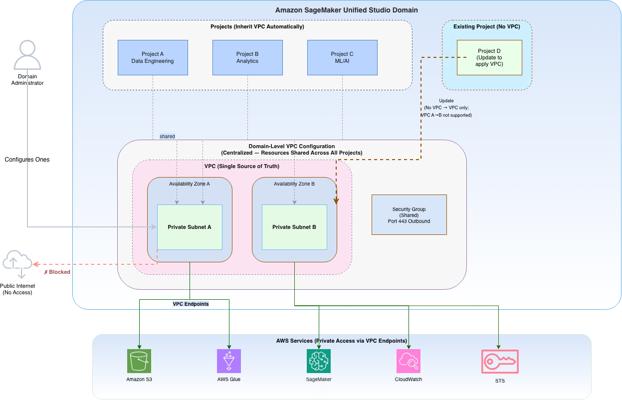
Figure 1: Domain-level VPC configuration in Amazon SageMaker Unified Studio. A single VPC with private subnets across two Availability Zones is configured at the domain level. All projects (data engineering, analytics, ML) inherit this configuration automatically
Key benefits of this approach:
Configure once, apply across projects: New projects inherit the domain VPC without manual intervention.
Consistent security posture: A single network boundary covers all data, analytics, and ML workloads.
Simplified auditing: One VPC to audit rather than one per project. Turn on VPC Flow Logs and review AWS CloudTrail events for network-level auditing.
Reduced operational overhead: Project teams start working immediately without submitting networking requests.
The following AWS services are used in this solution:
Before configuring domain-level VPC networking, verify you have the following:
Domain administrator permissions for Amazon SageMaker Unified Studio.
An existing VPC with the following requirements:
At least two private subnets in different Availability Zones.
DNS hostnames and DNS support enabled.
At least five available IP addresses per expected Amazon SageMaker Unified Studio project. This is a baseline minimum. Workloads using AWS Glue, Amazon EMR, or Amazon Redshift Serverless consume additional elastic network interfaces (ENIs) per worker or node. We recommend /24 or larger subnets for production domains and forward-looking capacity planning based on your expected users and compute types. For detailed guidance, see How to set up a network-isolated VPC for Amazon SageMaker Unified Studio.
VPC endpoints configured for the AWS services your projects access (for example, Amazon S3, AWS Glue, Amazon SageMaker AI).
Private DNS enabled on all interface VPC endpoints (you must enable this so that service DNS names resolve to private IPs). If you use centralized VPC endpoints through AWS Resource Access Manager (AWS RAM) or AWS Transit Gateway, configure Amazon Route 53 Resolver inbound endpoints instead.
S3 gateway endpoint route table associations configured for all selected private subnets (without this, S3 access fails in subnets whose route table lacks the prefix-list route).
A security group (optional), if not provided, SageMaker Unified Studio creates one automatically.
The SageMakerStudioAdminIAMConsolePolicy managed policy (or equivalent permissions including ec2:Describe*, ec2:CreateSecurityGroup, and datazone:* actions) attached to the domain administrator IAM role. See SageMakerStudioAdminIAMConsolePolicy in the AWS Managed Policy Reference for the full permission set.
Note: The VPC must be in the same AWS Region as the domain.
Because your subnets are private (no internet gateway route), compute resources access AWS services through VPC endpoints. At a minimum, configure the following interface and gateway endpoints (add Amazon Athena, AWS Lake Formation, or Amazon Redshift endpoints if you use them in your projects):
Endpoint
Type
Purpose
com.amazonaws.region.s3
Gateway
S3 access for data storage
com.amazonaws.region.glue
Interface
AWS Glue job connectivity
com.amazonaws.region.sagemaker.api
Interface
SageMaker API calls
com.amazonaws.region.sagemaker.runtime
Interface
Model inference
com.amazonaws.region.logs
Interface
Amazon CloudWatch Logs
com.amazonaws.region.monitoring
Interface
Amazon CloudWatch metrics
com.amazonaws.region.sts
Interface
IAM role assumption
com.amazonaws.region.datazone
Interface
Amazon SageMaker Unified Studio service connectivity
com.amazonaws.region.ecr.api
Interface
ECR API calls (container image metadata)
com.amazonaws.region.ecr.dkr
Interface
ECR image layer pulls (Docker registry)
com.amazonaws.region.kms
Interface
AWS Key Management Service (AWS KMS) encryption/decryption operations
Note: Interface endpoints incur an hourly charge per Availability Zone plus data processing fees. Gateway endpoints (such as S3) have no hourly charge. Factor endpoint count and AZ spread into your cost estimate.
Note: Review your account’s service quotas for interface VPC endpoints per VPC (default 50) and ENIs per Region before scaling. Request increases through Service Quotas if needed.
Solution walkthrough
The following steps walk you through configuring the domain VPC and validating it, from signing in to the console through confirming private connectivity from a project.
Step 1: Sign in and navigate to networking settings
Sign in to the AWS Management Console as your Amazon SageMaker Unified Studio domain administrator (the IAM role designated as the domain login role).
Use the Region selector in the top navigation bar to select the Region where your domain exists.
On the Amazon SageMaker Unified Studio landing page, choose Open to launch your IAM-based domain.
The following screenshot shows the Amazon SageMaker Unified Studio landing page, where you choose Open to launch the domain.
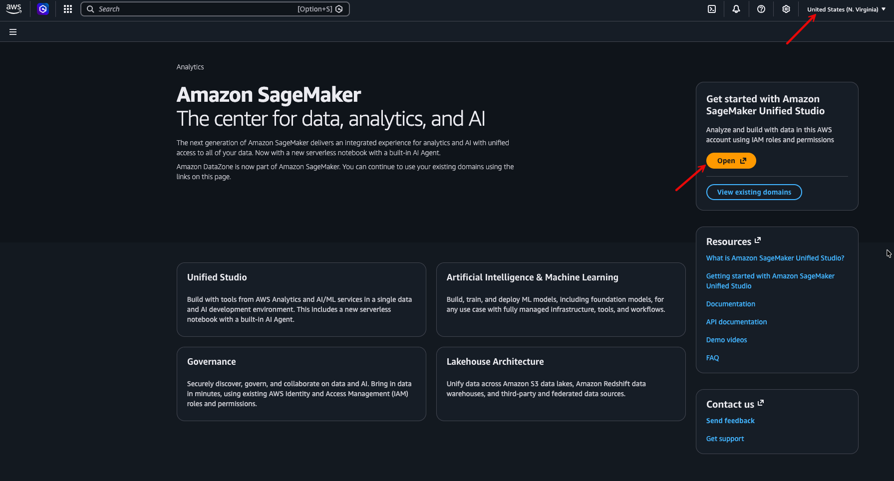
Figure 2: Amazon SageMaker Unified Studio landing page with the Open button to launch the IAM-based domain
From the navigation pane, choose Domain management.
The following screenshot shows Domain management in the navigation pane.
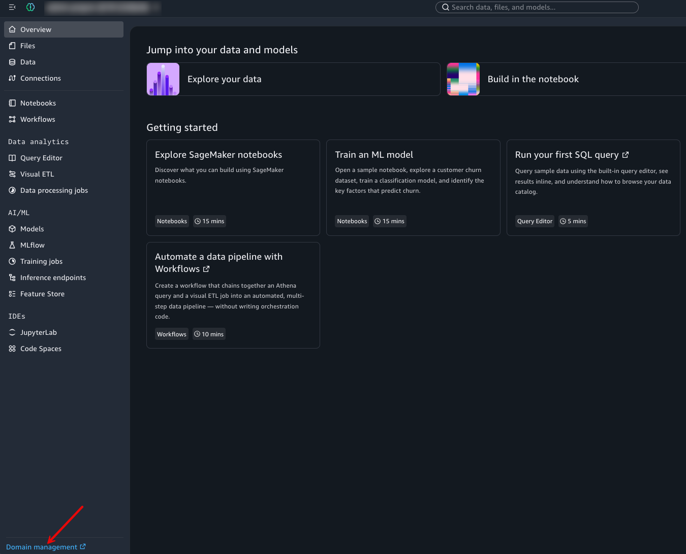
Figure 3: Domain management on navigation pane
Note: Access to the domain administration page is restricted to the IAM role specified as the domain login role during domain creation.
Step 2: Add VPC configuration
In the navigation pane, choose Settings. In the Networking in this account section, choose Add VPC.
The following screenshot shows the Networking in this account section with the Add VPC button.
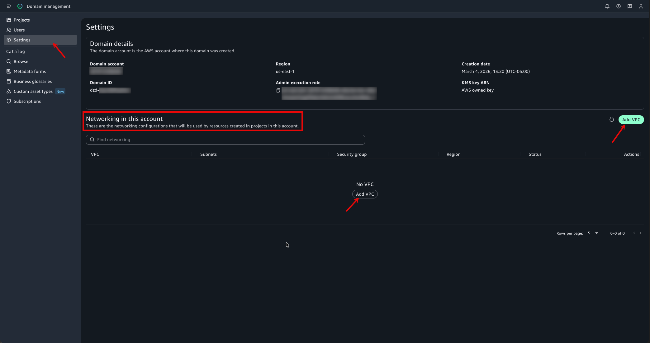
Figure 4: Domain management Settings page showing the Networking in this account section to add a VPC
For VPC, select the VPC with connectivity to your compute, database, and storage resources. If no VPC exists, choose Create VPC to provision one using AWS CloudFormation.
For Subnets, select a minimum of two private subnets in different Availability Zones.
(Optional) For Security group, select a security group to control inbound and outbound traffic. If you don’t choose one, SageMaker Unified Studio creates one automatically.
Choose Save.
Verify the VPC configuration status shows Ready in the Networking in this account section.
The following screenshots show the Add VPC dialog and the resulting Ready status in the Networking in this account section.
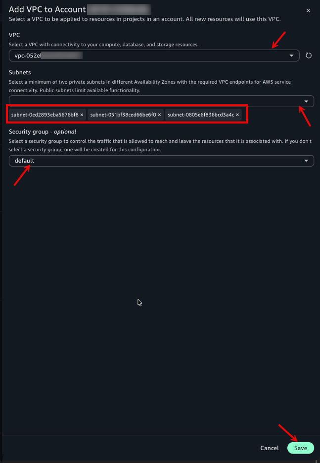
Figure 5: Add VPC dialog with fields for VPC, subnets, and security group selection

Figure 6: VPC configuration status showing Ready in the Networking in this account section
New projects created in the domain now automatically use the saved VPC configuration. Existing projects are an exception. See Step 3 to update them.
Step 3: Update existing projects
Existing projects don’t automatically inherit the domain VPC configuration. How you apply the new settings depends on the project’s current state:
Projects with no VPC configured – Update in place to adopt the domain VPC. See the following steps.
Projects that already have a VPC – These can’t be switched to a different VPC configuration. To adopt the domain VPC:
Create a new project (which inherits the domain VPC automatically).
Recreate connections in the new project.
Migrate assets from the old project.
Back up any data you need, then delete the original project.
Because recreation can disrupt in-progress work and doesn’t migrate project data automatically, schedule this as a planned maintenance window.
To update a project that currently has no VPC configured:
From the domain administration page, choose Projects in the navigation pane.
Choose the project you want to update.
On the project detail page, a banner appears: “Configurations have changed. Please update this project to access the latest configuration.”
In the banner, choose Update.
Confirm the update when prompted.
Repeat this process for each existing project that should use the domain VPC. The following screenshot shows the project detail page with the configuration update banner.
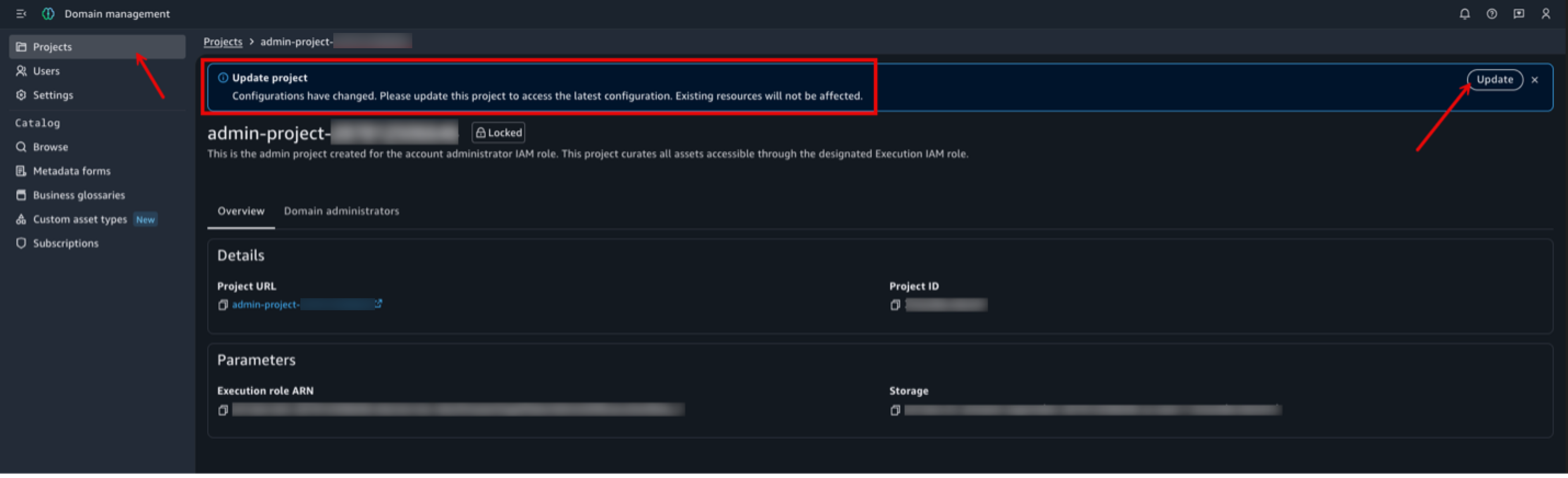
Figure 7: Project detail page showing the configuration update banner
Step 4: Validate connectivity
After configuring the domain VPC and updating your projects, verify connectivity. Compute resources should have private connectivity to AWS services through the VPC, without any additional project-level network configuration.
Create a notebook in one of your projects as shown in the following figure and run the following code:
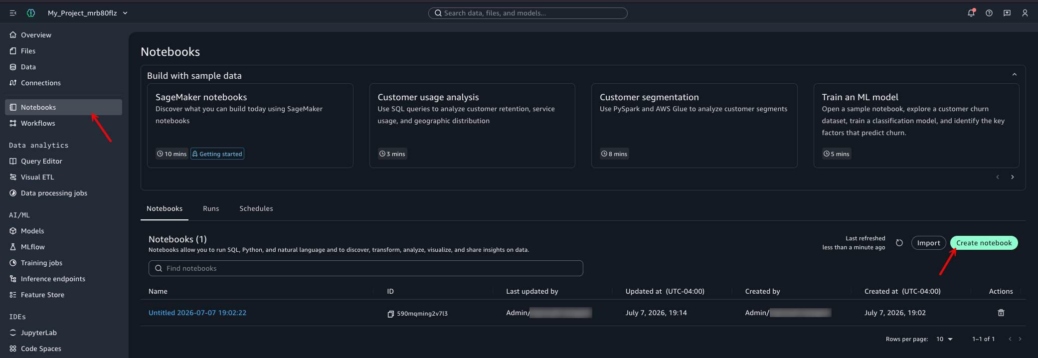
Figure 8: Creating a notebook in a SageMaker Unified Studio project to validate VPC connectivity
Requirements: Python 3.8+, Boto3 1.26 or later. Run in a notebook within your SageMaker Unified Studio project.
import boto3
import socket
import ipaddress
def validate_vpc_connectivity():
"""Validate that the project has private connectivity to AWS services
through the domain-level VPC configuration."""
results = {}
region = boto3.session.Session().region_name
if not region:
raise RuntimeError('Could not determine AWS Region. Run this notebook inside a SageMaker Unified Studio project.')
# Test Amazon S3 access via VPC endpoint
try:
s3 = boto3.client('s3')
response = s3.list_buckets()
results['S3'] = f"[PASS] Accessible ({len(response['Buckets'])} buckets)"
except Exception as e:
results['S3'] = f"[FAIL] Failed: {e}"
# Test AWS Glue access via VPC endpoint
try:
glue = boto3.client('glue')
dbs = glue.get_databases()
results['Glue'] = f"[PASS] Accessible ({len(dbs['DatabaseList'])} databases)"
except Exception as e:
results['Glue'] = f"[FAIL] Failed: {e}"
# Test STS (role assumption through VPC endpoint)
try:
sts = boto3.client('sts')
identity = sts.get_caller_identity()
results['STS'] = f"[PASS] Accessible (Account: {identity['Account']})"
except Exception as e:
results['STS'] = f"[FAIL] Failed: {e}"
# Verify interface endpoint resolves to private IP
try:
sts_endpoint = f"sts.{region}.amazonaws.com"
addr_info = socket.getaddrinfo(sts_endpoint, 443, family=socket.AF_INET)
ip = addr_info[0][4][0]
is_private = ipaddress.ip_address(ip).is_private
if is_private:
results['DNS Resolution'] = f"[PASS] Private IP ({ip}) (traffic stays on AWS network)"
else:
results['DNS Resolution'] = f"[WARN] Public IP ({ip}) - check VPC endpoint config"
except Exception as e:
results['DNS Resolution'] = f"[FAIL] Failed: {e}"
# Print results
print("-" * 40)
print("Domain VPC Connectivity Validation")
print("-" * 40)
for service, status in results.items():
print(f" {service}: {status}")
print("-" * 40)
print(f"\n Region: {region}")
# Check if all tests passed
all_passed = all("[PASS]" in status for status in results.values())
has_warn = any("[WARN]" in status for status in results.values())
if all_passed:
print(f"\n [PASS] All services accessible via private VPC endpoints.")
print(f" This project inherited its network configuration")
print(f" from the domain without per-project setup.")
elif has_warn and all("[PASS]" in s or "[WARN]" in s for s in results.values()):
print(f"\n [WARN] Services are reachable, but DNS resolves to public IPs.")
print(f" Verify that Private DNS is enabled on your interface VPC endpoints.")
else:
print(f"\n [FAIL] Some services are not reachable.")
print(f" Check that VPC endpoints are configured and security")
print(f" groups allow outbound traffic on port 443.")
validate_vpc_connectivity()
Expected output when VPC is correctly configured:
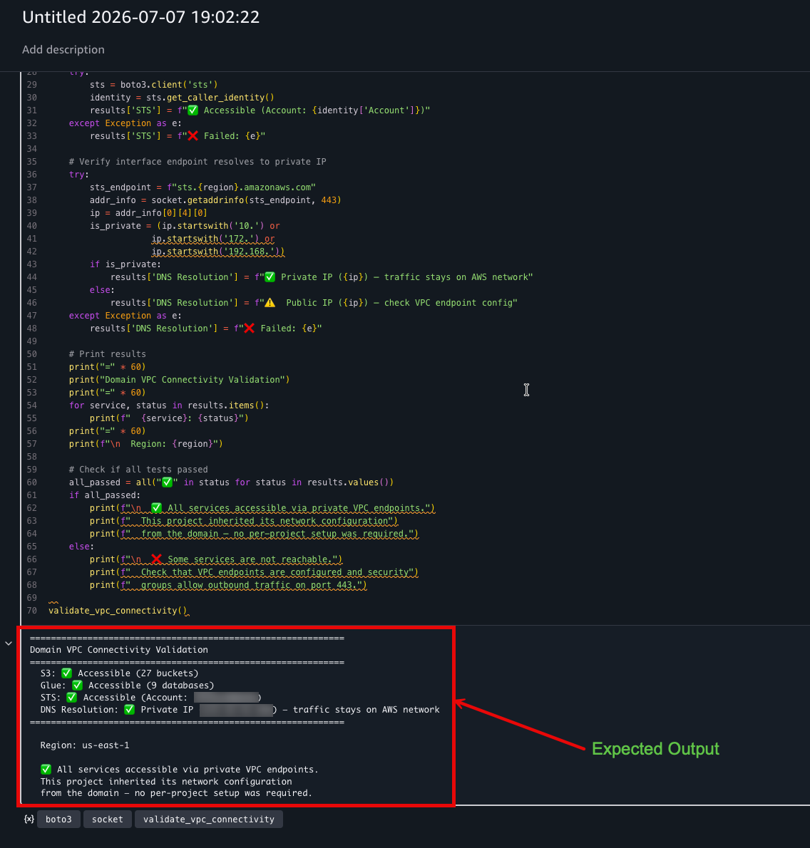
Figure 9: Successful validation output showing all services accessible through private VPC endpoints
If any service shows a failure, one common cause is security groups preventing traffic on port 443 to the VPC endpoint. Other causes include missing VPC endpoints, incorrect route table entries, or DNS resolution issues. For more information, see Configure VPC networking for IAM-based domains in the SageMaker Unified Studio Administrator Guide.
Note: An AccessDenied error indicates the request reached the service. Connectivity is working, but IAM permissions need adjustment (for example, the S3 test requires s3:ListAllMyBuckets, which some project roles lack). A timeout or connection error points to a networking problem (missing endpoint, route, or security group rule). The following screenshot shows the validation output when VPC endpoints are missing, where the affected services report timeout errors.
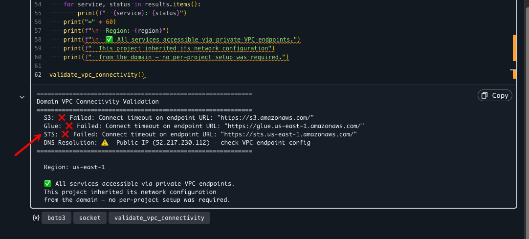
Figure 10: Validation output when VPC endpoints are not configured. Timeout errors indicate missing endpoints
The security group applied at the domain level controls network access for all projects. To review or tighten the rules:
Choose Security groups and choose the security group shown in your domain’s Networking settings.
Review the Inbound rules and Outbound rules tabs.
By default, the auto-created security group allows all outbound traffic on port 443 (HTTPS) to reach AWS services through VPC endpoints. Consider restricting outbound rules to only the specific VPC endpoint security groups for least-privilege access. Additionally, make sure your VPC endpoint security groups allow inbound TCP 443 from the domain security group or subnet CIDRs. For distributed compute services (AWS Glue, Amazon EMR), add a self-referencing inbound rule to allow worker-to-worker communication.
Updating VPC configuration
After the initial setup, you can modify the VPC configuration to change the VPC, subnets, or security group:
From the domain administration page, choose Settings in the navigation pane.
In the Networking in this account section, under the Actions column, choose Update.
Update the VPC, subnets, or security group as needed.
Choose Update.
The following screenshot shows the Update VPC dialog, where you modify the VPC, subnets, or security group.
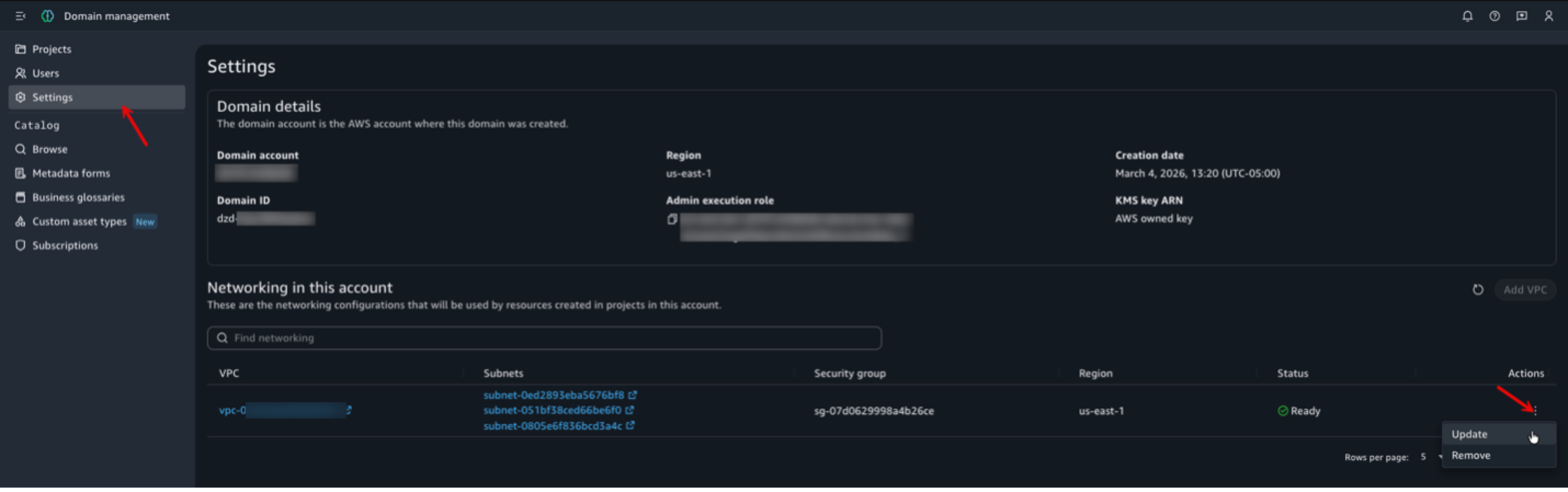
Figure 11: Update VPC dialog showing the option to modify VPC, subnets, or security group for the domain
Important: Updating the VPC does not affect already provisioned resources. Newly created resources in projects use the updated VPC. Existing projects that already have a VPC keep their original settings and must be recreated to adopt the change. Projects with no VPC can be updated in place (see Step 3).
Clean up
To remove the VPC configuration from your domain:
From the domain administration page, choose Settings in the navigation pane.
In the Networking in this account section, choose the Actions menu (⋮) and choose Remove.
The following screenshot shows the Actions menu with the Remove option.
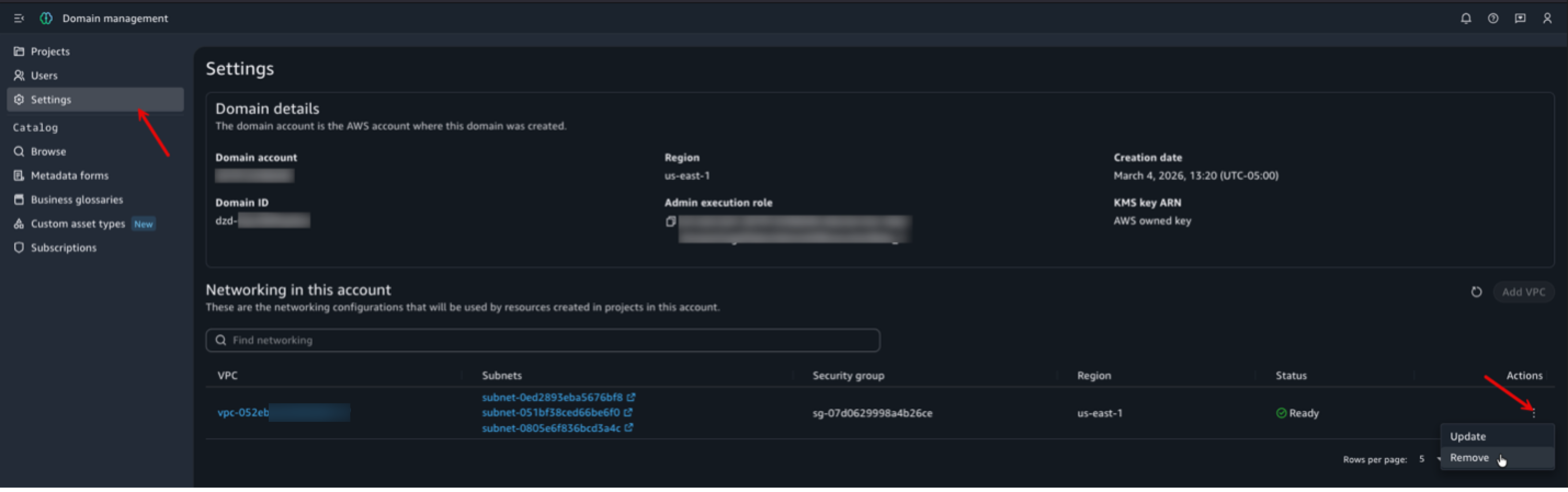
Figure 12: Actions menu in the Networking in this account section showing the Remove option
If you created a dedicated VPC for this walkthrough and no longer need it:
Delete the VPC and associated resources (subnets, VPC endpoints, security groups) from the Amazon VPC console. Before deleting, remove the domain VPC configuration and make sure all project resources are terminated. Active projects create ENIs that block VPC and subnet deletion.
If you used an AWS CloudFormation template to create the VPC, delete the stack to remove all resources cleanly. Open the AWS CloudFormation console and delete the stack.
Note: Removing the domain VPC configuration does not retroactively change projects that already have VPC applied. Those projects retain their existing network configuration. New projects created after removal do not have a VPC configured.
Conclusion
In this post, we showed how to configure domain-level VPC networking in Amazon SageMaker Unified Studio. A single domain-level VPC eliminates per-project networking overhead, enforces a consistent security posture, and simplifies compliance auditing.
Key takeaways:
Domain-level VPC is a one-time configuration that automatically applies to all new projects.
Projects with no VPC can be updated in place. Projects that already have a VPC must be recreated to adopt a changed configuration.
Private subnets with VPC endpoints provide secure, private connectivity to AWS services without traversing the public internet.
As next steps, consider:
Reviewing your auto-created security group rules and tightening them for least-privilege access.
Adding VPC endpoints for additional AWS services as your projects’ needs evolve.
Monitoring subnet IP address utilization to plan capacity as you add more projects. Use the AvailableIpAddressCount Amazon CloudWatch metric for your subnets to track utilization and set alarms.
If you run search on Amazon CloudSearch, now is the time to plan your migration to Amazon OpenSearch Serverless. Modern search has moved on to capabilities beyond what CloudSearch provides: semantic and hybrid search, Retrieval Augmented Generation (RAG), and agentic search. OpenSearch Serverless gives you all of these with automatic scaling on a pay-for-what-you-use basis. You don’t need to choose or maintain infrastructure. OpenSearch Serverless maintains the hands-off, operational simplicity of CloudSearch.
This post shows you how to migrate your CloudSearch domain to an Amazon OpenSearch Serverless collection. We walk you through assessing your CloudSearch configuration, creating an OpenSearch Serverless collection with explicit index mappings, converting your documents and queries, configuring security policies, loading your data with Amazon OpenSearch Ingestion, and validating the migration before cutting over.
Key differences to note
Independent scaling – OpenSearch Serverless scales indexing and search compute independently and can scale compute to zero when a collection is idle (you still pay for storage). For the cost structure, see Managing capacity limits for Amazon OpenSearch Serverless.
Layered security model – OpenSearch Serverless applies encryption, network, and data access policies at separate layers. For the security model, see Security in Amazon OpenSearch Serverless.
Prerequisites
To follow along with this post, you need the following:
An AWS account.
An existing Amazon CloudSearch domain with indexed data.
Source data available in a durable store such as Amazon Simple Storage Service (Amazon S3) or Amazon DynamoDB (CloudSearch doesn’t provide a built-in export or backup feature, so your original source data is required to re-ingest into OpenSearch).
AWS Identity and Access Management (IAM) permissions to create and manage Amazon OpenSearch Serverless collections, encryption policies, network policies, and data access policies.
An Amazon OpenSearch Ingestion pipeline (or alternative ingestion method) for loading data.
Plan the migration
Planning is where you decide what success means: minimal downtime, no data loss, current functionality preserved, and custom configurations carried over. You don’t need to plan for infrastructure because OpenSearch Serverless provisions and scales compute for you. Your main planning task is to assess your current CloudSearch configuration so you can reproduce its behavior on the target.
Document your existing setup from the Amazon CloudSearch console. Record the current instance type, the partition count, and the replication count. Capture the total document count and overall data size, and record every field definition, including field types and the search, facet, and sort settings for each field. Note any analyzers, synonyms, stopwords, or custom rank expressions. Note whether you use the 2011 or the 2013 CloudSearch API version, because the 2013 API added faceting and filtering features that change how you model the target.
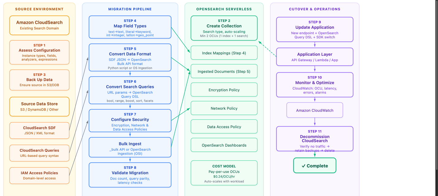
The migration involves four main concerns: your source data format, your queries, your field definitions, and your access policies. Before you plan the details, it helps to see the whole migration at once. The following diagram maps the migration across four phases: your source CloudSearch environment, the migration pipeline that converts and moves your data, the OpenSearch Serverless target, and cutover and operations.
Figure 1: The migration workflow across four phases
In the source environment, you assess your CloudSearch configuration and back up your source data (Amazon S3, Amazon DynamoDB, or another store). Note the Source Data Format (SDF), the URL-based query syntax, and the IAM access policies you need to carry over. In the migration pipeline, you map field types, convert the data format from CloudSearch JSON to OpenSearch-compatible JSON, convert your queries to the OpenSearch query domain-specific language (DSL), configure security, bulk-ingest the data, and validate the result. The OpenSearch Serverless target holds the collection, index mappings, ingested documents, and the encryption, network, and data access policies, and it scales with your workload on a pay-per-use basis. In cutover and operations, you update your application to the new endpoint and clients, monitor with Amazon CloudWatch, and decommission CloudSearch once no traffic remains.
Model your data in OpenSearch Service
OpenSearch Service uses index mappings to define the fields and data types in an index. Because you know your CloudSearch schema, define the target mapping explicitly when you create the index. Create the index and set its mapping in a single request, and set dynamic to strict so OpenSearch rejects any document that contains a field you did not define. Strict mapping catches schema drift at ingest time, avoiding the default OpenSearch behavior of creating new mappings for undefined fields.
The following table maps CloudSearch field types to their OpenSearch Service equivalents.
CloudSearch
OpenSearch Service equivalent
Notes
text
text
Text is tokenized. Stemming, synonyms, and stopwords apply. Good for matching user terms.
literal
keyword
Not tokenized. Good for exact-match search.
int
integer
Use for ranking, faceting, and narrowing.
double
float or double
.
date
date
.
boolean
boolean
.
latlon
geo_point
.
text-array
text
OpenSearch handles arrays natively, so map to the base text type.
literal-array
keyword
OpenSearch handles arrays natively, so map to the base keyword type.
multi-value
nested or object
.
long
long
.
binary
binary
.
Two mapping details deserve attention. First, pick the smallest numeric type that fits your data rather than copying the widths CloudSearch uses. CloudSearch stores integers as 64-bit values, but few datasets hold numbers that large. A long or a double consumes more disk than an integer, a short, or a float with no benefit when the values are small. Evaluate the actual range of each field and choose the narrowest type that holds it. Reserve long for values that genuinely exceed the roughly 2.1 billion ceiling of integer, and use float instead of double unless you need double precision. Smaller types shrink your index and speed up queries.
Second, if you sort or aggregate on a text field, add a keyword sub-field. The preceding example mapping has a keyword subfield for the title field. You access the field using dot notation: title.keyword. OpenSearch doesn’t sort or aggregate analyzed text fields by default.
As noted earlier, if you run several CloudSearch domains, model each one as a separate index within a single OpenSearch Serverless collection to consolidate them.
Move your data
Migrating to OpenSearch Service is a re-ingestion: you convert your source documents and index them into the collection you created. CloudSearch doesn’t provide a built-in backup or snapshot feature. It relies on the documents you send through the indexing process, so before you migrate, make sure your source data is available in a durable store such as Amazon S3, Amazon DynamoDB, or another database.
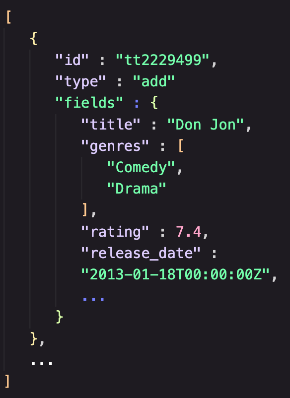
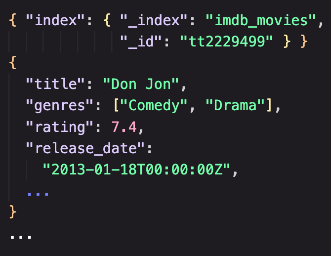
The conversion is a format translation. CloudSearch accepts data in SDF as JSON or XML, where a document batch is a collection of add and delete operations. The JSON that CloudSearch uses differs from the JSON that OpenSearch Service expects, so you must transform each source document into an OpenSearch document whose fields match the index mapping you defined earlier. Handle the same details the mapping calls out: emit each numeric value so it fits the narrow type you chose for its field rather than a wide long or double, format dates to match your date mapping, and drop or rename any field that your strict mapping doesn’t define.
Figure 2: CloudSearch batch format (left) compared to OpenSearch batch format (right)
You can write a small conversion script. Have the script write its output to an Amazon S3 bucket so the converted documents live in a durable store you can re-ingest from as many times as you need.
With your converted documents in Amazon S3, use Amazon OpenSearch Ingestion to load them. Amazon OpenSearch Ingestion is a feature of Amazon OpenSearch Service that you can use to ingest, filter, transform, enrich, and route data to an Amazon OpenSearch Service domain or an OpenSearch Serverless collection. Configure an OpenSearch Ingestion pipeline with an Amazon S3 source (you can use an OpenSearch Ingestion blueprint to get started) that reads your converted documents. Let its built-in processors apply any final transformation before the pipeline writes to your collection. A managed pipeline reading from Amazon S3 gives you a repeatable, restartable load without operating ingestion infrastructure, which makes it the recommended path for most migrations.
If you prefer to load data directly, OpenSearch Service exposes a REST API, so you can index documents with a standard client such as curl or with the OpenSearch client libraries for many languages. Direct indexing is convenient for a small dataset or a quick test, but an Amazon S3 source with OpenSearch Ingestion is the better choice for a production migration.
Convert your queries
CloudSearch uses a URL-based query format. You pass a query parameter in the URL and submit either a simple string search or a JSON-formatted query. OpenSearch Service uses a REST API and the OpenSearch query DSL in the request body, which gives you compound queries, function scoring, and richer relevance control. You can use generative AI coding assistants to help with this translation. Provide your CloudSearch query patterns, and the model generates the equivalent OpenSearch query DSL, which you then validate against your test cases.
Query syntax changes
CloudSearch appends parameters such as sort to the query URL, while OpenSearch expresses sorting, filtering, and boosting as explicit elements of the request body. For example, a title search for “shakespeare” in CloudSearch looks like the following.
To keep result sets consistent after migration, set the default operator to AND in OpenSearch to match the default query behavior of CloudSearch. The following table shows common CloudSearch query patterns and their OpenSearch Service equivalents, using a sample IMDB movies dataset.
Boosting is useful when you want certain fields or terms to carry more weight in relevance scoring. A higher boost value means the term contributes more to the score. OpenSearch also supports sorting by _score (relevance), which is the default when you specify no sort. For the full query language, see the OpenSearch query DSL documentation.
Configure security
CloudSearch uses AWS Identity and Access Management policies to control access to its configuration and domain service APIs. You attach user-based policies to an IAM role, user, or group, and the document, search, and suggest actions in those policies control access to the CloudSearch APIs.
OpenSearch Serverless applies security through policies at several layers.
Collections: Encrypted at rest by default, using either an AWS owned key or a customer managed key defined in an encryption policy.
Network policies: Define whether a collection is reachable privately through a virtual private cloud (VPC) endpoint or over the internet.
Data access policies: Control which IAM principals and Security Assertion Markup Language (SAML) identities can create indexes and read or write data in the collection.
Amazon OpenSearch Service provisioned domains also offer fine-grained access control, with role-based access control and security at the index, document, and field level. For OpenSearch Serverless, data access policies provide collection-level and index-level permissions, controlling which IAM principals and SAML identities can create, read, or write data within a collection.
Validate the migration
Validation confirms that the migration is complete and correct before you send production traffic to OpenSearch Serverless. Work through five kinds of validation.
Documents: Check your document count. Your OpenSearch Serverless indexes should have the same count as your CloudSearch indexes.
Queries: Translate your most important queries and run them manually against your collection. Spot check the output for the presence of important results.
Ranking: Check the order of results, especially for queries with custom rank functions or field weighting. Results might not match exactly, so look for anything that’s incorrect.
Latency: Ideally you should tee your production traffic to your Serverless collection to get real latency metrics. Worst case, generate at least 100,000 synthetic queries across all your query types and run them. Monitor OpenSearch Compute Unit (OCU) consumption with Amazon CloudWatch to understand your cost profile.
To validate search functionality, run the same query against both systems and compare the results. Reuse the query pairs from the conversion step so you exercise the syntax differences directly. For example, to check a numeric range against the sample IMDB movies dataset, run the following query in CloudSearch.
https://my-cloudsearch-domain.us-east-1.cloudsearch.amazonaws.com/2013-01-01/search?q=rating: [7 TO 9]&size=10
Run the equivalent query DSL against your OpenSearch Serverless collection.
Confirm that both queries return the same set of movies. Then repeat the comparison for a query that exercises relevance, such as the boosted query from the conversion step, and confirm the top results appear in the same order.
When validation passes, update your application to use the OpenSearch Serverless endpoint and the query DSL, and switch from the CloudSearch SDK to the OpenSearch client libraries. After cutover, confirm that no application still points to a CloudSearch endpoint, retain your source data backups in Amazon S3 for rollback, and then delete the CloudSearch domain.
Operating OpenSearch Serverless in production is lighter than operating a domain, because OpenSearch Serverless scales compute for you and you do not tune shards, instance types, or capacity. Your focus shifts to cost and search quality. Monitor OCU consumption and search latency with Amazon CloudWatch, and set alarms on the thresholds that matter to you. Review OCU usage patterns to understand cost and find optimization opportunities, and set capacity limits on the collection to cap the maximum OCUs it can consume. For guidance, see Managing capacity limits for Amazon OpenSearch Serverless and Monitoring Amazon OpenSearch Serverless.
Cost considerations
With OpenSearch Serverless, you pay only for the compute and storage your workload consumes, and OpenSearch Serverless charges for compute and storage separately. OpenSearch Serverless scales indexing compute and search compute independently, so a write-heavy or a read-heavy workload scales only the dimension it needs, and compute can scale to zero when a collection is idle, in which case you pay only for storage. To share hardware across workloads, place collections in a collection group so they draw from the same compute rather than each provisioning its own. For pricing and unit details, see Amazon OpenSearch Service pricing.
Clean up
Because you’re migrating to OpenSearch Serverless, the resources that you’ve created will likely become your production resources. If not, delete any OpenSearch Serverless collections and S3 buckets you created to avoid incurring ongoing cost.
Conclusion
In this post, you saw how Amazon CloudSearch and Amazon OpenSearch Serverless compare, and how the concepts you rely on in CloudSearch (field types, query syntax, autoscaling, and access control) translate into OpenSearch Service. You assess your CloudSearch configuration, model your data with explicit OpenSearch mappings, move your converted documents into the collection with OpenSearch Ingestion, convert your URL-based queries into the OpenSearch query DSL, configure security, and validate before cutover. OpenSearch Serverless gives you the hands-off operational model you have with CloudSearch, and adds richer query capabilities, granular data access policies, and automatic scaling. To get started, create an OpenSearch Serverless collection on the AWS Management Console and follow the steps in this post.
Upgrading PySpark jobs to a new Apache Spark major version can introduce breaking changes. Removed configuration keys, stricter type casting, and Python library incompatibilities can cause runtime failures or silent behavior differences. With AWS Glue 6.0 now running Apache Spark 4.1 and Python 3.13, you need a reliable way to migrate your existing jobs while validating correctness.
In this post, we walk through upgrading a PySpark ETL job from AWS Glue 5.1 to AWS Glue 6.0. We use the generative AI upgrades for Apache Spark in the AWS Glue console. The upgrade analysis automatically identifies incompatibilities, iteratively resolves them, validates the result with data quality checks, and presents recommended changes for your review. AWS Glue 6.0 also delivers up to 36% better price performance* along with Iceberg v3, Spark Declarative Pipelines, Real-Time Mode, and Arrow-native Python UDFs.
What changes with AWS Glue 6.0
AWS Glue 6.0 runs Apache Spark 4.1, which introduces several behavioral changes from the Spark 3.5 runtime used in AWS Glue 5.1:
Behavior
Spark 3.5 (AWS Glue 5.1)
Spark 4.1 (AWS Glue 6.0)
ANSI SQL mode
Disabled by default
Enabled by default
Legacy Parquet datetime configs
Supported
Removed (renamed)
Python runtime
3.11
3.13
Beyond version compatibility, AWS Glue 6.0 also introduces:
Apache Iceberg v3 with VARIANT Shredding for efficient semi-structured data handling.
Arrow-native Python UDFs (PyArrow) for improved performance.
Built-in observability with structured metrics and enhanced Spark UI.
Up to 36% better price performance compared to AWS Glue 5.1*.
These runtime changes mean your existing AWS Glue jobs might encounter removed configuration keys, stricter type casting behavior, or Python package version incompatibilities when running on AWS Glue 6.0. Fixing these manually is time-consuming and error-prone. The following sections show how the generative upgrade analysis handles this automatically.
The sample job
Our example is a daily ecommerce order analytics pipeline running on AWS Glue 5.1:
What the job does:
Ingests 10,000 orders from Parquet files with INT96 timestamps (including pre-1900 historical dates from a legacy system migration).
Computes revenue metrics by casting string prices to numeric values and calculating line totals with discounts and tax.
Segments customers using recency, frequency, and monetary (RFM) scoring through mapInPandas with pandas and scikit-learn.
This job runs successfully on AWS Glue 5.1. The following sections walk through how the upgrade analysis identifies and resolves incompatibilities when upgrading this job to AWS Glue 6.0. Before starting, confirm you have the prerequisites in place.
Prerequisites
An AWS account with access to the AWS Glue console.
An existing AWS Glue job on version 5.1 or earlier with at least one successful run.
An Amazon S3 path for storing the upgrade analysis results.
Running the upgrade analysis from the console
The following steps walk through the upgrade analysis workflow using the AWS Glue console.
Step 1: Select your job
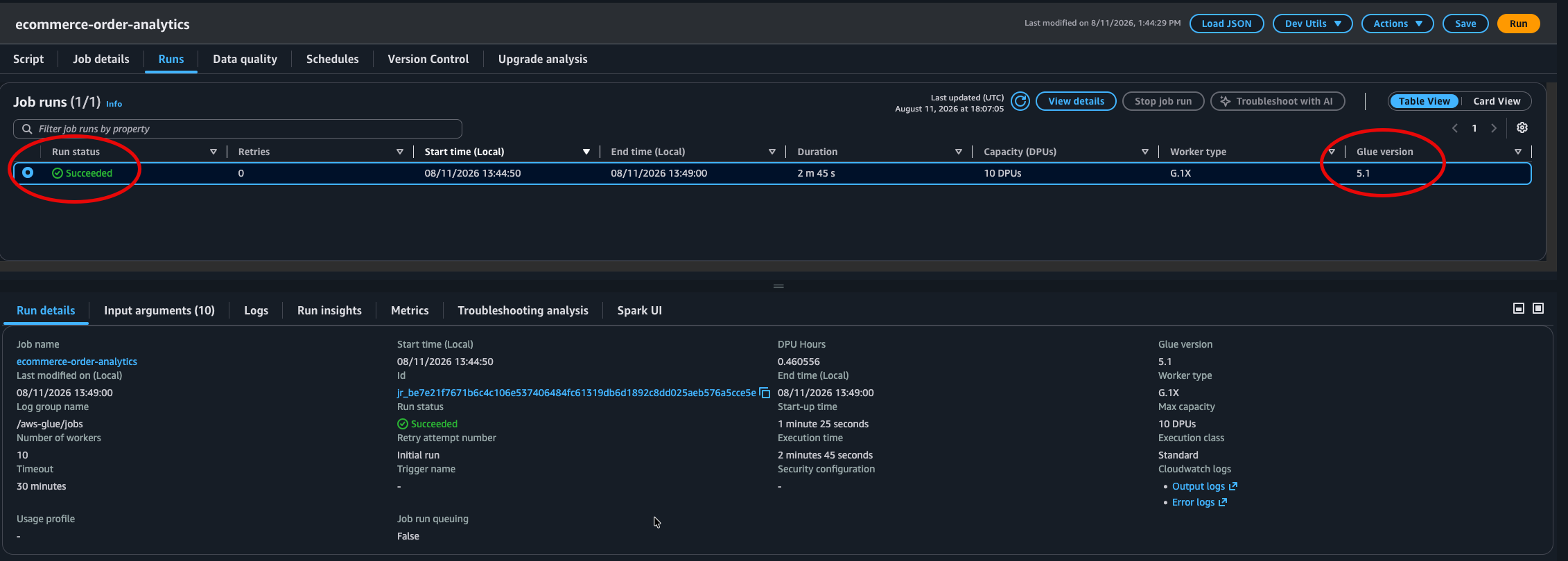
Navigate to your job in the AWS Glue Studio console. Confirm the job has a successful run history on AWS Glue 5.1 before starting the upgrade analysis.
Figure 1: Job run status for the job on AWS Glue 5.1
Step 2: Start the upgrade analysis
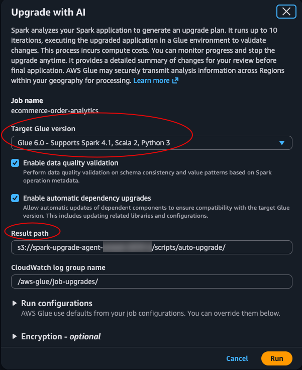
From the job’s Actions menu, select Upgrade with generative AI. Configure the following:
Target AWS Glue version: 6.0.
Results S3 path: An S3 location where the analysis stores its artifacts and recommendations.
Figure 2: The Upgrade with generative AI option in the Actions menu
Configure the target AWS Glue version and the S3 results path, then choose Run.
Figure 3: The Upgrade with generative AI window for setting the target AWS Glue version and results path
Choose Run. The analysis begins by running your job on AWS Glue 5.1 to establish a baseline. It then iteratively tests the job on AWS Glue 6.0, identifies failures, applies recommended fixes, and validates the job. If the upgrade analysis cannot resolve an incompatibility within its attempt budget, the analysis stops and reports the unresolved issue for manual review. Your original job remains unchanged.
Note: The upgrade analysis executes your job multiple times (one baseline run plus one or more validation attempts), and each run consumes Data Processing Units (DPUs). For large or long-running jobs, consider using the run configuration option to specify fewer workers or a smaller dataset to optimize analysis cost.
Step 3: Monitor progress
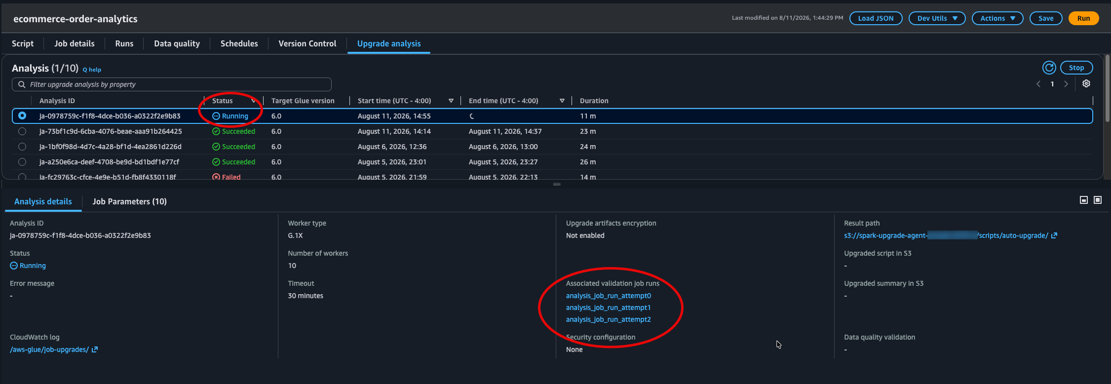
The console displays the analysis progressing through multiple validation attempts. Each attempt either succeeds or fails with a specific error, and the upgrade analysis uses that error signal to determine and apply the appropriate fix for the next attempt.
Figure 4: Upgrade analysis progress across multiple validation attempts
What the upgrade analysis found and fixed
The analysis completed in four validation attempts, identifying and resolving three distinct incompatibilities. The upgrade uses deterministic migration rules for known config changes, and automated diagnosis for runtime or code errors.
Iteration 1: Removed Parquet legacy configuration
The analysis first sanitizes any Spark configurations that were removed in Spark 4.1. Our job used spark.sql.legacy.parquet.datetimeRebaseModeInWrite and spark.sql.legacy.parquet.int96RebaseModeInWrite, which no longer exist.
Migration rule applied: The SQL configs with the spark.sql.legacy prefix were removed in Spark 4.1. They have been renamed to their non-legacy equivalents, preserving the original values.
The read-side configs (datetimeRebaseModeInRead, int96RebaseModeInRead) already used the correct non-legacy names and required no changes.
However, with this fix applied, the validation run still failed because the Python module installation encountered an error on the AWS Glue 6.0 image.
Iteration 2: Python module version incompatibility
The pinned module versions (pandas==2.2.2, scikit-learn==1.5.0, numpy==1.26.4) could not be installed in the AWS Glue 6.0 Python 3.13 environment.
Error:
LAUNCH ERROR | Installation of Additional Python Modules failed
Recommended change: The upgrade analysis updated the version specifications from exact pins to minimum version constraints, allowing pip to resolve compatible versions for Python 3.13:
With modules installing successfully, the job launched on AWS Glue 6.0 but encountered a runtime error.
Iteration 3: ANSI mode strict type casting
Spark 4.1 enables ANSI SQL mode by default (spark.sql.ansi.enabled=true). Our revenue calculation casts string prices to double, but approximately 1.8% of records contain non-numeric placeholder values such as “N/A”, “pending”, or “null” from the upstream system. From a business perspective, this meant 1.8% of revenue orders were silently excluded from revenue metrics. This data quality issue was invisible to the original pipeline.
On AWS Glue 5.1 (ANSI mode off), cast("N/A" as double) silently returns null. On AWS Glue 6.0 (ANSI mode on), this throws an exception:
Error:
NumberFormatException: [CAST_INVALID_INPUT] The value 'null' of the type
"STRING" cannot be cast to "DOUBLE" because it is malformed. Correct the
value as per the syntax, or change its target type. Use try_cast to
tolerate malformed input and return NULL instead. SQLSTATE: 22018
Migration rule applied: As of Spark 4.1, spark.sql.ansi.enabled is on by default. Casting a malformed value now raises CAST_INVALID_INPUT instead of returning NULL. The upgrade analysis resolved this by updating the script to use try_cast(), which safely returns NULL for malformed input while preserving ANSI mode protections for the rest of the job.
Recommended change:
Before (AWS Glue 5.1):
F.col("unit_price").cast("double")
After (AWS Glue 6.0, fixed by the upgrade analysis):
F.expr("try_cast(unit_price as double)")
This is a targeted fix that handles the known dirty data without disabling ANSI mode globally, keeping overflow detection and type safety active throughout the job.
Final validation and data quality check
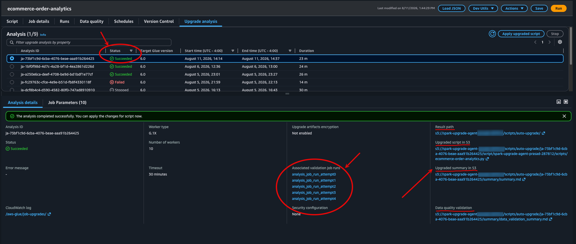
After applying all three fixes, the analysis ran the job on AWS Glue 6.0 one final time and performed a data quality comparison between the AWS Glue 5.1 baseline output and the AWS Glue 6.0 output.
Result: The job completed successfully and all data validations passed with no mismatches detected between the source and target outputs.
Figure 5: Final analysis status with links to the results output path in Amazon S3
Reviewing the upgrade summary
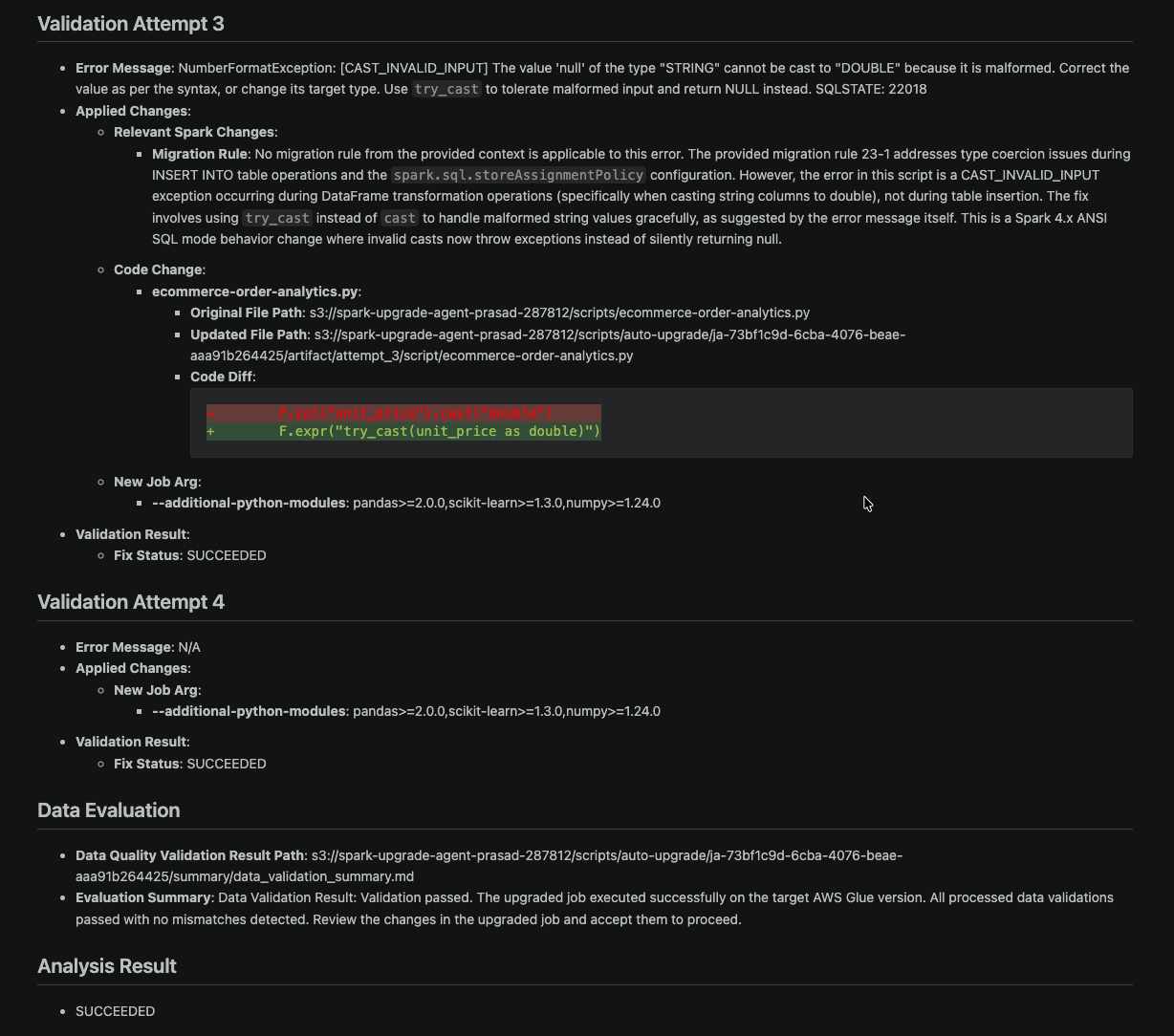
The analysis produces a detailed summary stored in your S3 results path. This summary documents each validation attempt, the errors encountered, the migration rules applied, and the recommended configuration changes:
The following is a snippet from the upgrade summary (summary.md) showing the recommended changes and validation attempt details:
The summary documents each validation attempt, the changes applied, and the data quality results.
Figure 6: Upgrade summary snippet showing validation attempt details, data quality, and analysis results
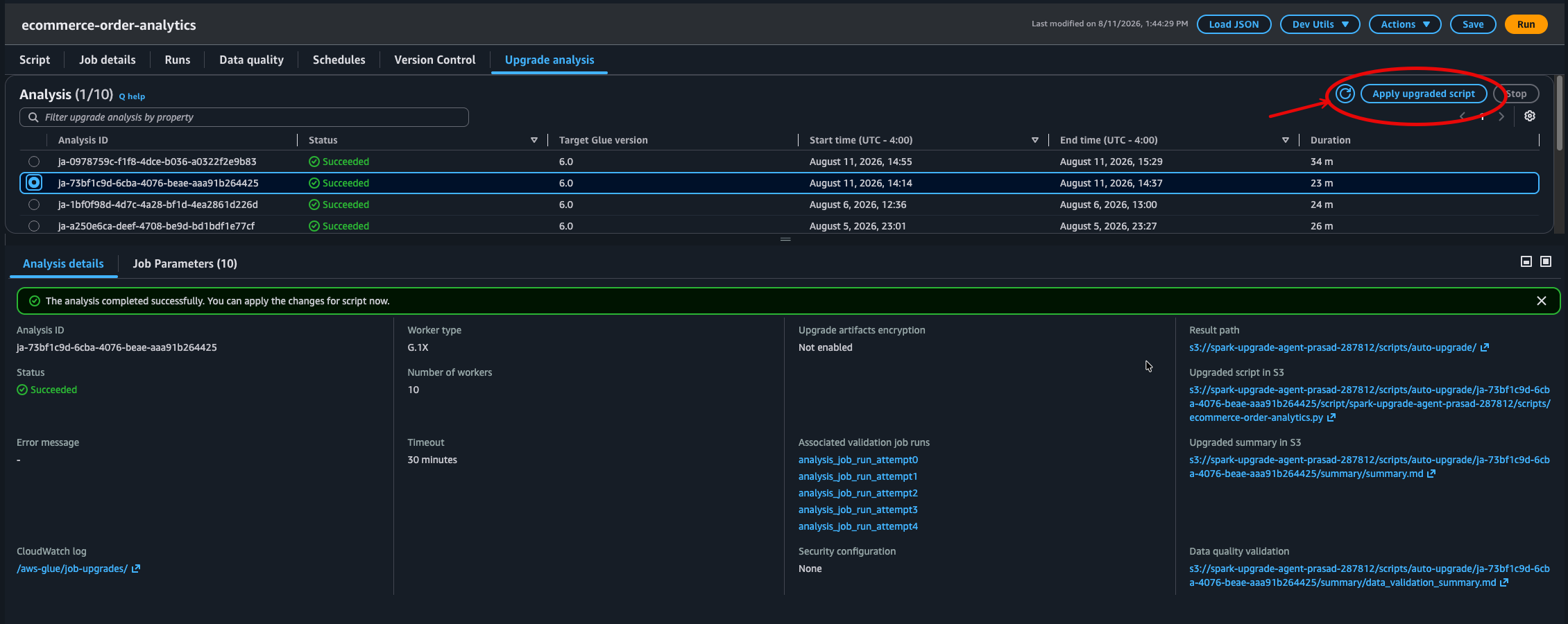
After reviewing the recommendations, accept the changes to upgrade your job to AWS Glue 6.0. This updates your job definition with the recommended configuration, including the renamed Spark configs, updated module versions, and any script modifications. Because the analysis has already validated the job on AWS Glue 6.0 and confirmed data quality parity with the original, your job is ready for production.
After reviewing the recommendations, you can apply the upgraded script to your job.
Figure 7: The option to apply the upgraded script to the job
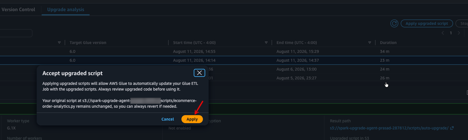
Choose Apply to confirm the upgrade.
Figure 8: The Apply button that confirms upgrading the job to AWS Glue 6.0
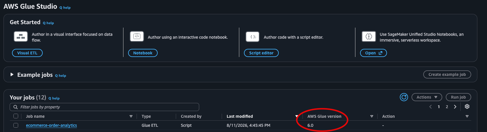
After applying, the job definition reflects the new AWS Glue version.
Figure 9: The AWS Glue version for the job after applying the upgrade
Python virtual environments in AWS Glue 6.0
AWS Glue 6.0 introduces --python-virtual-env-storage-prefix, a service-managed virtual environment with S3 caching that simplifies Python dependency management.
For existing jobs that use --additional-python-modules, no action is required. AWS Glue automatically handles the conversion to virtual environments when your job runs on AWS Glue 6.0. Your jobs continue to work without any changes.
For new jobs on AWS Glue 6.0, we recommend using the virtual environment approach:
On the first run, AWS Glue installs your modules into a virtual environment, packages it, and caches the result to your specified S3 path (approximately 15–30 seconds of additional startup time).
On subsequent runs, AWS Glue downloads and extracts the cached virtual environment instead of running pip install.
The cache is automatically invalidated when your module list, versions, or AWS Glue version changes.
This approach provides faster cold starts after the first run, requires no Docker image management (unlike --python-virtual-env), and is entirely service-managed with no maintenance burden.
Conclusion
The generative upgrade analysis identified and resolved three distinct compatibility issues in our AWS Glue 5.1 job, so the job now runs successfully on AWS Glue 6.0 with Apache Spark 4.1:
The upgrade analysis renamed legacy Parquet datetime configuration keys (removed in Spark 4.1) to their current equivalents.
The upgrade analysis updated Python module version specifications that were incompatible with Python 3.13 to use flexible minimum version constraints.
The upgrade analysis addressed the new ANSI SQL mode default (which causes runtime failures on malformed data) with a targeted fix using try_cast() to safely handle non-numeric values while preserving ANSI mode protections.
The analysis validated that the upgraded job produces output consistent with the original, and presented all changes as recommendations for review before applying them to your job.
To reproduce this walkthrough, start with any existing AWS Glue job running on version 5.1 or earlier with a successful run history. No additional sample code or CloudFormation template is required.
After you have reviewed and accepted the upgrade changes, you can delete the analysis results stored in your S3 results path.
*Based on 3TB TPC-DS benchmark comparing AWS Glue 6.0 to AWS Glue 5.1.
Upgrading Apache Spark applications across major versions means tracking down breaking changes, manually debugging failures from log files, and running repeated test cycles. This process can stretch across weeks for complex code bases.
In this post, we walk through a hands-on PySpark migration from Spark 3.5 to Spark 4.0 on Amazon EMR Serverless, using the AWS Spark Upgrade Agent. You’ll see how the agent iteratively validates your application on a live Amazon EMR Serverless application, automatically diagnosing and resolving failures from Amazon CloudWatch logs until the job succeeds. By the end, you have a multi-pipeline PySpark application running on Spark 4.0 with four distinct breaking changes resolved. The fixes include configuration key removals, codec renames, and stricter charset validation, all driven through natural language interaction in the Integrated Development Environment (IDE).
This is part 2 of a three-part series on how the AWS Spark Upgrade Agent can automate and simplify Spark upgrades.
In Part 1, we introduced the agent’s architecture and capabilities. This post walks through a complete PySpark migration from Spark 3.5 to Spark 4.0 on Amazon EMR Serverless.
In the sections that follow, you will set up the prerequisites and infrastructure, explore the sample application, run the iterative validation workflow on EMR Serverless, review data quality results, and generate a comprehensive upgrade summary.
Note: Because this upgrade is performed using the AWS Spark Upgrade Agent Model Context Protocol (MCP) server, an agentic artificial intelligence (AI) system, the agent might take different paths to reach the same successful outcome. The workflow demonstrated here represents one successful upgrade path. The key takeaway is the end-to-end workflow: generating an upgrade plan, iteratively validating on Amazon EMR Serverless, and producing a comprehensive upgrade summary.
1. Prerequisites and setup
This section covers the tools, infrastructure, and IDE configuration you need before starting the upgrade. To follow along, you need an AWS account with an AWS Identity and Access Management (AWS IAM) user or role that has permissions to deploy AWS CloudFormation stacks, create AWS IAM roles and policies, and create Amazon EMR Serverless applications. Intermediate knowledge of AWS Command Line Interface (AWS CLI), AWS CloudFormation, and Python is helpful.
1.1 Install Kiro CLI and local tools
In this post, we use Kiro CLI to demonstrate the upgrade workflow. You can use an MCP-compatible IDE or framework. Examples include VS Code with Cline, Cursor, Windsurf, and Claude Desktop, among others. To follow along with Kiro CLI, install it on your workstation. For more details on the installation and setup, refer to Setup for Upgrade Agent:
curl -fsSL https://cli.kiro.dev/install | bash
Run the following command and use your builder ID to log in:
kiro-cli login --use-device-flow
With the Kiro CLI installed and logged in, rather than installing the remaining tools manually, use Kiro CLI to set up and verify your prerequisites with the following prompt:
kiro-cli chat
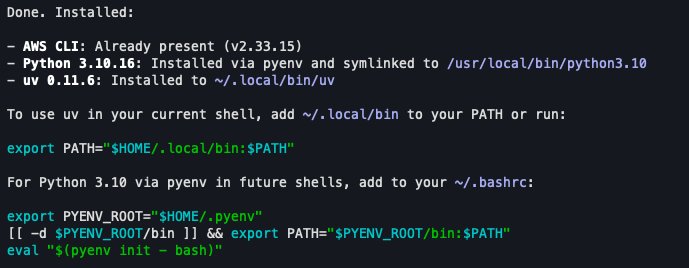
> Install AWS CLI, Python 3.10, and uv on my system if they are not already installed
Output of AWS CLI and local tools install step.
These tools are needed for the upgrade workflow:
AWS CLI: Configured with a profile that has permissions to assume the AWS Identity and Access Management (AWS IAM) role created following.
Python 3.10+: Required to match the EMR 8.0 runtime.
Two AWS CloudFormation stacks create the required resources: an AWS IAM role, an Amazon Simple Storage Service (Amazon S3) staging bucket, an Amazon EMR Serverless application (Spark 4.0.1), and its execution role.
Stack 1 – AWS IAM role and Amazon S3 staging bucket:
The spark-upgrade-mcp-setup template creates the AWS IAM role and Amazon S3 staging bucket required by the upgrade agent. Choose the Launch Stack button for your Region. For additional Regions, see the full region list.
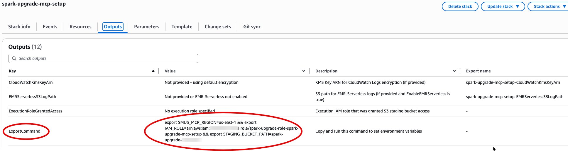
After deployment, open the AWS CloudFormation Outputs tab, copy the ExportCommand value, and run it in your terminal. This sets SMUS_MCP_REGION, IAM_ROLE, and STAGING_BUCKET_PATH automatically.
aws configure set profile.spark-upgrade-profile.role_arn ${IAM_ROLE}
aws configure set profile.spark-upgrade-profile.source_profile default
aws configure set profile.spark-upgrade-profile.region ${SMUS_MCP_REGION}
This creates two Amazon EMR Serverless applications: a source (Spark 3.5.0) for data quality baseline and a target (Spark 4.0.1) for upgrade validation, with a shared execution role. Both applications auto-stop after 15 minutes of idle time, so there is no cost when not in use. To upgrade between different Spark versions, override SourceReleaseLabel and TargetReleaseLabel with your target Amazon EMR release labels.
After the stack completes deployment, note the outputs:
For other MCP clients, refer to your IDE’s MCP configuration documentation and use the same server parameters shown previously.
Verify the connection: Start Kiro CLI and confirm the spark-upgrade tools are loaded:
$ kiro-cli chat
...
spark-upgrade (MCP):
- generate_spark_upgrade_plan * not trusted
- update_build_configuration * not trusted
- fix_upgrade_failure * not trusted
- run_validation_job * not trusted
- check_job_status * not trusted
...
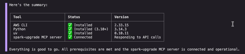
Tip: After Kiro CLI and the MCP server are configured, you can ask the agent to verify your setup. For example: “Check if I have AWS CLI, Python 3.10+, and uv installed, and confirm the spark-upgrade MCP server is connected.”
Output showing the status of each tool, AWS CLI, and MCP server.
Tip: Trust mode vs. confirm mode: When running the upgrade agent in Kiro CLI, you have two options:
Trust mode: Type t when prompted to approve a tool. The agent auto-approves subsequent uses of that tool without asking for confirmation. You can also use /tools trust-all to trust every tool at once for a fully autonomous experience.
Confirm mode: Type y for each individual tool invocation. This lets you review, verify, and approve every action before the agent runs it. If this is your first time using the agent, use confirm mode for full visibility.
2. Hands-on PySpark upgrade from Spark 3.5 to Spark 4.0
This section walks through the complete migration of a representative PySpark application from Amazon EMR Serverless 7.0.0 (Spark 3.5.0) to EMR Serverless with the emr-spark-8.0-preview release label (Spark 4.0.1), using the global_logistics_platform sample.
2.1 Sample project: global logistics platform
The sample application is a multi-domain PySpark data processing application with three pipelines:
Fleet management: Processes vehicle telemetry data (GPS tracking, fuel consumption, driver behavior scoring) using window functions, lag/lead operations, and statistical aggregations. Writes Parquet with lz4raw compression.
International shipping: Handles cross-border shipment documents with multi-language address standardization using character encoding functions (encode/decode with charsets like Shift_JIS, GB2312, EUC-KR), and processes carrier manifests with ISO-8859-1 encoding.
Historical compliance: Processes regulatory audit records spanning centuries (including pre-1582 Julian calendar dates), requiring legacy datetime rebasing for Parquet writes.
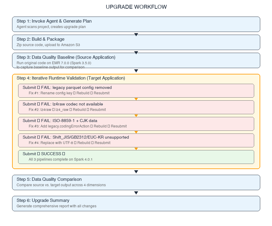
Before diving into the upgrade, here are the four specific breaking changes present in this code base that the agent discovers and resolves entirely through runtime validation:
#
Incompatibility
File(s)
1
Legacy Parquet configuration key removed:spark.sql.legacy.parquet.datetimeRebaseModeInWrite removed in Spark 4.0. Must use spark.sql.parquet.datetimeRebaseModeInWrite.
spark_config.py
2
Parquet compression codec rename:lz4raw codec renamed to lz4_raw in Spark 4.0.
telemetry_processor.py
3
Stricter charset encoding validation: Spark 4.0 tightened encode() behavior. Encoding CJK (Chinese, Japanese, Korean) characters to ISO-8859-1 now throws MALFORMED_CHARACTER_CODING. In Spark 3.x this silently replaced unmappable chars with ?. Restored via spark.sql.legacy.codingErrorAction.
spark_config.py
4
Character encoding restrictions:encode()/decode() in Spark 4.0 supports US-ASCII, ISO-8859-1, UTF-8, UTF-16BE, UTF-16LE, UTF-16, and UTF-32. Code uses Shift_JIS, GB2312, EUC-KR.
shipment_processor.py
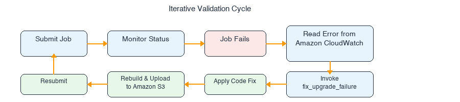
The agent resolves each of these through iterative runtime validation on EMR Serverless: submitting the job, diagnosing failures from Amazon CloudWatch logs, applying fixes, and resubmitting until the job succeeds.
2.3 Step 1: Invoke the upgrade agent
Open the project in Kiro CLI and enter the following prompt:
Upgrade my Spark application in the current directory from EMR serverless version 7.0.0 to EMR serverless version 8.0.0.
Use Amazon EMR Serverless target app-id <YOUR-TARGET-APP-ID> and execution role
<YOUR-EXECUTION-ROLE-ARN> for validation.
Use source Amazon EMR Serverless app-id <YOUR-SOURCE-APP-ID> for data quality baseline.
Store artifacts at s3://${STAGING_BUCKET_PATH}/spark4-upgrade/python/
Enable data quality validation
Tip: The SourceApplicationId, TargetApplicationId, and ExecutionRoleArn are in the Outputs of the spark-emr-serverless-upgrade AWS CloudFormation stack you deployed in Section 1.2.
The agent invokes generate_spark_upgrade_plan, scans the project structure, identifies the Spark version mapping (EMR 7.0.0 → Spark 3.5.0, EMR 8.0.0 → Spark 4.0.1), and produces a structured upgrade plan with an Analysis ID for traceability.
The agent presents the plan and asks for confirmation. Type y to approve the tool invocation, or t to trust that tool for the rest of the session.
You have an option to save the plan as a local JSON file for future reference or to resume the upgrade at a later point, so go ahead and ask Kiro to save it locally. Provide the AWS CLI profile that you have configured on your system. Use the following prompt to provide these inputs:
Yes I would like to save the plan to a local file and use spark-upgrade-profile
2.4 Step 2: Build and package
The agent validates the Python project compiles successfully, then packages it for Amazon EMR Serverless deployment:
Runs py_compile on each .py file to verify syntax.
Creates src.zip containing the src/ directory (preserving the import structure used by from src.utils import ...).
Uploads src.zip, main.py, and sample input data to the Amazon S3 staging path.
# What the agent does behind the scenes:
zip -r src.zip src/
aws s3 cp main.py s3://<YOUR-BUCKET>/spark4-upgrade/python/<ANALYSIS-ID>/source/main.py
aws s3 cp src.zip s3://<YOUR-BUCKET>/spark4-upgrade/python/<ANALYSIS-ID>/source/src.zip
aws s3 cp data/sample/ s3://<YOUR-BUCKET>/spark4-upgrade/python/<ANALYSIS-ID>/input/ --recursive
No external dependencies (no requirements.txt), so no virtual environment is needed. If your project has external dependencies in a requirements.txt, the agent will package them into a virtual environment archive and include it in the EMR Serverless submission parameters.
2.5 Step 3: Data quality baseline on source application
Before migrating the code, the agent establishes a data quality baseline by running the original (pre-upgrade) code on the source Amazon EMR Serverless application (Spark 3.5.0 / EMR 7.0.0). This captures the expected output that the upgraded application must match.
The agent submits the job to the source application with data quality check enabled:
The agent monitors the source run via check_job_status until it completes successfully. This baseline output is stored for comparison after the target validation succeeds.
2.6 Step 4: Iterative runtime validation on target application
This is the core of the upgrade. The agent submits the unmodified application to the target Amazon EMR Serverless application (Spark 4.0.1), and every incompatibility is discovered, diagnosed, and fixed through runtime failures. The agent drives the entire fix cycle by submitting to EMR, reading errors from Amazon CloudWatch logs, applying fixes, rebuilding, and resubmitting.
The agent presents the proposed Amazon EMR Serverless job configuration for your review before each submission. Type y to approve.
The first submission fails immediately at SparkSession initialization:
org.apache.spark.sql.AnalysisException:
The SQL config 'spark.sql.legacy.parquet.datetimeRebaseModeInWrite' was removed
in the version 4.0.0. Use 'spark.sql.parquet.datetimeRebaseModeInWrite' instead.
The Historical Compliance pipeline configures spark.sql.legacy.parquet.datetimeRebaseModeInWrite for handling pre-1582 Julian calendar dates. Spark 4.0 removed the legacy. prefix from this configuration key.
The agent calls fix_upgrade_failure, which identifies the migration rule and recommends the fix:
File:src/utils/spark_config.py
# Before
.config("spark.sql.legacy.parquet.datetimeRebaseModeInWrite", "LEGACY")
# After
.config("spark.sql.parquet.datetimeRebaseModeInWrite", "LEGACY")
After applying the fix, the agent rebuilds src.zip, re-uploads to Amazon S3, and resubmits the job.
The resubmitted job fails with a new error, which confirms progress:
pyspark.errors.exceptions.captured.IllegalArgumentException:
[CODEC_NOT_AVAILABLE.WITH_AVAILABLE_CODECS_SUGGESTION]
The codec lz4raw is not available.
Available codecs are brotli, uncompressed, lzo, snappy, lz4_raw, none, zstd, lz4, gzip.
SQLSTATE: 56038
The Fleet Management pipeline’s telemetry_processor.py uses lz4raw as the Parquet compression codec. Spark 4.0 renamed this to lz4_raw (with an underscore).
org.apache.spark.SparkRuntimeException:
[MALFORMED_CHARACTER_CODING]
Invalid value found when performing `encode` with ISO-8859-1
SQLSTATE: 22000
The International Shipping pipeline’s process_carrier_manifests() method uses encode(..., 'ISO-8859-1') on data containing CJK (Chinese, Japanese, Korean) characters. Although ISO-8859-1 is in Spark 4.0’s supported charset list, it is a single-byte encoding that cannot represent CJK characters. In Spark 3.x, the Java charset encoder silently replaced unmappable characters with ?. Spark 4.0 tightened this behavior to throw MALFORMED_CHARACTER_CODING for unmappable characters.
The agent identifies the migration rule and adds a legacy compatibility configuration:
File:src/utils/spark_config.py
# Added to SparkSession builder
.config("spark.sql.legacy.codingErrorAction", "true")
This restores the Spark 3.x behavior where unmappable characters are silently replaced instead of throwing errors.
With the configuration added, the agent rebuilds and resubmits.
2.6.4 Fix 4: Character encoding restrictions (iteration 4)
The fourth submission fails with yet another encoding error:
org.apache.spark.SparkIllegalArgumentException:
[INVALID_PARAMETER_VALUE.CHARSET]
The value of parameter(s) `charset` in `encode` is invalid:
expects one of the iso-8859-1, us-ascii, utf-16, utf-16be, utf-16le, utf-32, utf-8,
but got Shift_JIS. SQLSTATE: 22023
The International Shipping pipeline’s standardize_addresses_with_charset() method uses Shift_JIS, GB2312, and EUC-KR charsets in encode()/decode() calls. Spark 4.0 restricts these functions to seven standard charsets. These regional charsets are not in the supported list.
The agent replaces the unsupported charsets with UTF-8:
The three pipelines (Fleet Management, International Shipping, and Historical Compliance) complete on EMR Serverless with the emr-spark-8.0-preview release label (Spark 4.0.1).
2.7 Summary of the iterative runtime validation
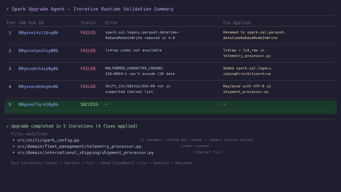
The runtime validation loop is the core value of the upgrade agent. Here’s the complete iteration history:
Each iteration follows the same cycle:
Failures that would normally require manual log analysis, root cause investigation, and code patching are resolved automatically by the agent in this workflow.
3. Data quality validation
With both the source baseline (Section 2.5) and the upgraded target run (Section 2.6) completed successfully, the agent performs data quality validation to verify the migration hasn’t changed your application’s output. This is the key advantage of including the source application in your upgrade prompt: the agent can compare outputs from both Spark versions side by side.
3.1 Data quality comparison
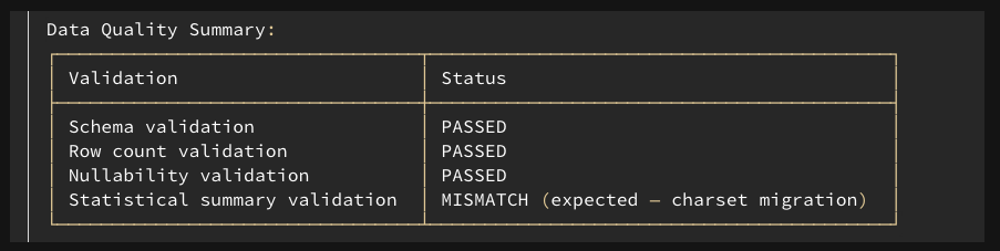
The agent invokes get_data_quality_summary to compare the outputs across four dimensions:
Schema validation: Confirms column names, data types, and column ordering match between source and target outputs.
Row count validation: Verifies no data loss or duplication during migration.
Nullability validation: Detects changes in null handling.
The preceding image shows the data quality summary.
Three of four checks pass cleanly. The statistical summary validation detects a mismatch in the shipper_address column of the customs_declarations output: the max and min summary values differ between source and target.
3.2 Understanding and resolving the mismatch
This mismatch is a direct consequence of Fix 4 (Section 2.6.4). The original code ran addresses through a Shift_JIS/GB2312/EUC-KR → UTF-8 roundtrip that produced garbled text, because the intermediate regional charset corrupted multi-byte UTF-8 characters. The upgraded code uses UTF-8 → UTF-8, preserving addresses faithfully. The mismatch reflects improved data quality, not a regression.
Schema, row counts, and nullability matched exactly: the difference is limited to string values that were previously garbled. No further action is needed. The upgraded application is production-ready.
Expected behavior: Character encoding migrations might change string values, although they preserve semantic meaning. When data quality validation reports mismatches, trace each one back to a specific code change. If the mismatch is explained by a required migration fix (as here), verify the new behavior is correct and document it. If a mismatch cannot be explained, investigate before promoting to production.
4. Upgrade summary
After the agent completes the entire upgrade workflow, it produces a comprehensive upgrade summary following a structured template. This summary lets you review the job configuration updates, code modifications with diffs and file references, relevant migration rules applied, and data quality validation status.
Here is the summary the agent produced for this upgrade:
Upgrade plan
Compile and build project with current Spark 3.5.0: validated that Python files compile successfully.
Run baseline validation on source EMR Serverless (00g4vhvt1lhtrs09) with Spark 3.5.0: established data quality baseline.
Run target validation on target EMR Serverless (00g4vhvt3np1bj09) with Spark 4.0.1: fixed 4 issues iteratively across 4 validation attempts.
Compare data quality between source and target runs: detected expected mismatch in shipper_address.
Generate and persist upgrade summary.
Upgrade result
Upgrade completed with data validation enabled. Data validation detected an expected mismatch in the shipper_address column because of the charset encoding migration from unsupported charsets (Shift_JIS, GB2312, EUC-KR) to UTF-8.
Dependency changes
No external dependencies were changed in this project (no requirements.txt).
Job configuration changes
Parquet datetime rebase configuration key renamed.
Migration rule: In Spark 4.0, the legacy datetime rebasing SQL configurations with the prefix spark.sql.legacy are removed. The SQL configuration spark.sql.legacy.parquet.datetimeRebaseModeInWrite was removed in the version 4.0.0. Use spark.sql.parquet.datetimeRebaseModeInWrite instead.
Legacy coding error action enabled.
Change: Added spark.sql.legacy.codingErrorAction set to true.
Migration rule: In Spark 4.0, the encode() and decode() functions raise MALFORMED_CHARACTER_CODING error when handling unmappable characters. In Spark 3.5 and earlier versions, these characters are replaced with garbled text. To restore the previous behavior, set spark.sql.legacy.codingErrorAction to true.
Error: [INVALID_PARAMETER_VALUE.CHARSET] charset in encode is invalid: expects one of iso-8859-1, us-ascii, utf-16, utf-16be, utf-16le, utf-32, utf-8, but got Shift_JIS.
Applied changes: src/domain/international_shipping/shipment_processor.py: Replaced Shift_JIS, GB2312, EUC-KR with UTF-8 for shipper and consignee address encoding.
Data mismatch: 1. The shipper_address column max summary value changed in customs_declarations output. This is expected because of the charset encoding migration from Shift_JIS/GB2312/EUC-KR to UTF-8. 2. The shipper_address column min summary value changed in customs_declarations output for the same expected cause.
5. Conclusion
The AWS Spark Upgrade Agent turns a traditionally time-consuming PySpark migration into an automated, iterative workflow. For the Global Logistics Platform sample, the agent identified and resolved four distinct Spark 4.0 breaking changes: legacy Parquet configuration key removal, compression codec renames, stricter charset encoding validation, and character encoding restrictions. Each fix was applied across three domain processors, through natural language interaction in the IDE.
Every incompatibility was discovered through runtime validation on Amazon EMR Serverless. The agent submitted the unmodified application to the target application, and each failure revealed the next breaking change:
The spark.sql.legacy.parquet.datetimeRebaseModeInWrite configuration removal, which crashes SparkSession initialization.
The lz4raw → lz4_raw codec rename, which fails when Parquet writes run.
ISO-8859-1 encoding of CJK characters: ISO-8859-1 is a valid Spark 4.0 charset, so the failure surfaces only when the code runs against real multi-language data, because Spark 4.0 tightened charset encoding validation to reject unmappable characters.
Shift_JIS/GB2312/EUC-KR charsets removed from Spark 4.0’s supported charset list entirely.
The agent diagnosed each error from Amazon CloudWatch logs, applied the fix, rebuilt, and resubmitted without manual intervention beyond approving each step. The data quality validation then confirmed that the upgraded application produces equivalent output on Spark 4.0.1: schema, row counts, and nullability matched exactly. The one difference, in the shipper_address column, resulted from the charset migration from regional encodings to UTF-8, which actually improved data quality by eliminating garbled text from incorrect encoding roundtrips. With each mismatch traced back to a specific, understood code change, the upgraded application is production-ready.
Hundreds of thousands of organizations build data integration pipelines to extract and transform data. They establish data quality rules to ensure the extracted data is of high quality for accurate business decisions. These rules assess the data based on fixed criteria reflecting current business states. However, when the business environment changes, data properties shift, rendering these fixed criteria outdated and causing poor data quality.
For example, a data engineer at a retail company established a rule that validates daily sales must exceed a 1-million-dollar threshold. After a few months, daily sales surpassed 2 million dollars, rendering the threshold obsolete. The data engineer couldn’t update the rules to reflect the latest thresholds due to lack of notification and the effort required to manually analyze and update the rule. Later in the month, business users noticed a 25% drop in their sales. After hours of investigation, the data engineers discovered that an extract, transform, and load (ETL) pipeline responsible for extracting data from some stores had failed without generating errors. The rule with outdated thresholds continued to operate successfully without detecting this issue. The ordering system that used the sales data placed incorrect orders, causing low inventory for future weeks. What if the data engineer had the ability to set up dynamic thresholds that automatically adjusted as business properties changed?
We are excited to talk about how to use dynamic rules, a new capability of AWS Glue Data Quality. Now, you can define dynamic rules and not worry about updating static rules on a regular basis to adapt to varying data trends. This feature enables you to author dynamic rules to compare current metrics produced by your rules with your historical values. These historical comparisons are enabled by using the last(k) operator in expressions. For example, instead of writing a static rule like RowCount > 1000, which might become obsolete as data volume grows over time, you can replace it with a dynamic rule like RowCount > min(last(3)) . This dynamic rule will succeed when the number of rows in the current run is greater than the minimum row count from the most recent three runs for the same dataset.
This is part 7 of a seven-part series of posts to explain how AWS Glue Data Quality works. Check out the other posts in the series:
Part 7: Get started with AWS Glue Data Quality dynamic rules for ETL pipelines
Previous posts explain how to author static data quality rules. In this post, we show how to create an AWS Glue job that measures and monitors the data quality of a data pipeline using dynamic rules. We also show how to take action based on the data quality results.
Solution overview
Let’s consider an example data quality pipeline where a data engineer ingests data from a raw zone and loads it into a curated zone in a data lake. The data engineer is tasked with not only extracting, transforming, and loading data, but also identifying anomalies compared against data quality statistics from historical runs.
In this post, you’ll learn how to author dynamic rules in your AWS Glue job in order to take appropriate actions based on the outcome.
The data used in this post is sourced from NYC yellow taxi trip data. The yellow taxi trip records include fields capturing pickup and dropoff dates and times, pickup and dropoff locations, trip distances, itemized fares, rate types, payment types, and driver-reported passenger counts. The following screenshot shows an example of the data.
Set up resources with AWS CloudFormation
This post includes an AWS CloudFormation template for a quick setup. You can review and customize it to suit your needs.
The CloudFormation template generates the following resources:
An AWS Lambda which will create the following folder structure within the above Amazon S3 bucket:
raw-src/
landing/nytaxi/
processed/nytaxi/
dqresults/nytaxi/
AWS Identity and Access Management (IAM) users, roles, and policies. The IAM role GlueDataQuality-* has AWS Glue run permission as well as read and write permission on the S3 bucket.
To create your resources, complete the following steps:
Leave all the other settings as their default values.
Choose Save.
After the job is saved, navigate to the Visual tab and on the Sources menu, choose Amazon S3.
In the Data source properties – S3 pane, for S3 source type, select S3 location.
Choose Browse S3 and navigate to the prefix /landing/nytaxi/ in the S3 bucket starting with gluedataqualitydynamicrules-*.
For Data format, choose Parquet and choose Infer schema.
On the Transforms menu, choose Evaluate Data Quality.
You now implement validation logic in your process to identify potential data quality problems originating from the source data.
To accomplish this, specify the following DQDL rules on the Ruleset editor tab:
CustomSql "select vendorid from primary where passenger_count > 0" with threshold > 0.9,
Mean "trip_distance" < max(last(3)) * 1.50,
Sum "total_amount" between min(last(3)) * 0.8 and max(last(3)) * 1.2,
RowCount between min(last(3)) * 0.9 and max(last(3)) * 1.2,
Completeness "fare_amount" >= avg(last(3)) * 0.9,
DistinctValuesCount "ratecodeid" between avg(last(3))-1 and avg(last(3))+2,
DistinctValuesCount "pulocationid" > avg(last(3)) * 0.8,
ColumnCount = max(last(2))
Select Original data to output the original input data from the source and add a new node below the Evaluate Data Quality node.
Choose Add new columns to indicate data quality errors to add four new columns to the output schema.
Select Data quality results to capture the status of each rule configured and add a new node below the Evaluate Data Quality node.
With rowLevelOutcomes node selected, choose Amazon S3 on the Targets menu.
Configure the S3 target location to /processed/nytaxi/ under the bucket name starting with gluedataqualitydynamicrules-* and set the output format to Parquet and compression type to Snappy.
With the ruleOutcomes node selected, choose Amazon S3 on the Targets menu.
Configure the S3 target location to /dqresults/ under the bucket name starting with gluedataqualitydynamicrules-*.
Set the output format to Parquet and compression type to Snappy.
Choose Save.
Up to this point, you have set up an AWS Glue job, specified dynamic rules for the pipeline, and configured the target location for both the original source data and AWS Glue Data Quality results to be written on Amazon S3. Next, let’s examine dynamic rules and how they function, and provide an explanation of each rule we used in our job.
Dynamic rules
You can now author dynamic rules to compare current metrics produced by your rules with their historical values. These historical comparisons are enabled by using the last() operator in expressions. For example, the rule RowCount > max(last(1)) will succeed when the number of rows in the current run is greater than the most recent prior row count for the same dataset. last() takes an optional natural number argument describing how many prior metrics to consider; last(k) where k >= 1 will reference the last k metrics. The rule has the following conditions:
If no data points are available, last(k) will return the default value 0.0
If fewer than k metrics are available, last(k) will return all prior metrics
For example, if values from previous runs are (5, 3, 2, 1, 4), max(last (3)) will return 5.
AWS Glue supports over 15 types of dynamic rules, providing a robust set of data quality validation capabilities. For more information, refer to Dynamic rules. This section demonstrates several rule types to showcase the functionality and enable you to apply these features in your own use cases.
CustomSQL
The CustomSQL rule provides the capability to run a custom SQL statement against a dataset and check the return value against a given expression.
The following example rule uses a SQL statement wherein you specify a column name in your SELECT statement, against which you compare with some condition to get row-level results. A threshold condition expression defines a threshold of how many records should fail in order for the entire rule to fail. In this example, more than 90% of records should contain passenger_count greater than 0 for the rule to pass:
CustomSql "select vendorid from primary where passenger_count > 0" with threshold > 0.9
Note: Custom SQL also supports Dynamic rules, below is an example of how to use it in your job
CustomSql "select count(*) from primary" between min(last(3)) * 0.9 and max(last(3)) * 1.2
Mean
The Mean rule checks whether the mean (average) of all the values in a column matches a given expression.
The following example rule checks that the mean of trip_distance is less than the maximum value for the column trip distance over the last three runs times 1.5:
Mean "trip_distance" < max(last(3)) * 1.50
Sum
The Sum rule checks the sum of all the values in a column against a given expression.
The following example rule checks that the sum of total_amount is between 80% of the minimum of the last three runs and 120% of the maximum of the last three runs:
Sum "total_amount" between min(last(3)) * 0.8 and max(last(3)) * 1.2
RowCount
The RowCount rule checks the row count of a dataset against a given expression. In the expression, you can specify the number of rows or a range of rows using operators like > and <.
The following example rule checks if the row count is between 90% of the minimum of the last three runs and 120% of the maximum of last three runs (excluding the current run). This rule applies to the entire dataset.
RowCount between min(last(3)) * 0.9 and max(last(3)) * 1.2
Completeness
The Completeness rule checks the percentage of complete (non-null) values in a column against a given expression.
The following example rule checks if the completeness of the fare_amount column is greater than or equal to the 90% of the average of the last three runs:
Completeness "fare_amount" >= avg(last(3)) * 0.9
DistinctValuesCount
The DistinctValuesCount rule checks the number of distinct values in a column against a given expression.
The following example rules checks for two conditions:
If the distinct count for the ratecodeid column is between the average of the last three runs minus 1 and the average of the last three runs plus 2
If the distinct count for the pulocationid column is greater than 80% of the average of the last three runs
DistinctValuesCount "ratecodeid" between avg(last(3))-1 and avg(last(3))+2,
DistinctValuesCount "pulocationid" > avg(last(3)) * 0.8
ColumnCount
The ColumnCount rule checks the column count of the primary dataset against a given expression. In the expression, you can specify the number of columns or a range of columns using operators like > and <.
The following example rule check if the column count is equal to the maximum of the last two runs:
ColumnCount = max(last(2))
Run the job
Now that the job setup is complete, we are prepared to run it. As previously indicated, dynamic rules are determined using the last(k) operator, with k set to 3 in the configured job. This implies that data quality rules will be evaluated using metrics from the previous three runs. To assess these rules accurately, the job must be run a minimum of k+1 times, requiring a total of four runs to thoroughly evaluate dynamic rules. In this example, we simulate an ETL job with data quality rules, starting with an initial run followed by three incremental runs.
First job (initial)
Complete the following steps for the initial run:
Navigate to the source data files made available under the prefix /raw-src/ in the S3 bucket starting with gluedataqualitydynamicrules-*.
To simulate the initial run, copy the day one file 20220101.parquet under /raw-src/ to the /landing/nytaxi/ folder in the same S3 bucket.
On the AWS Glue Studio console, choose ETL Jobs in the navigation pane.
Choose GlueDataQualityDynamicRule under Your jobs to open it.
Choose Run to run the job.
You can view the job run details on the Runs tab. It will take a few minutes for the job to complete.
After job successfully completes, navigate to the Data quality -updated tab.
You can observe the Data Quality rules, rule status, and evaluated metrics for each rule that you set in the job. The following screenshot shows the results.
The rule details are as follows:
CustomSql – The rule passes the data quality check because 95% of records have a passenger_count greater than 0, which exceeds the set threshold of 90%.
Mean – The rule fails due to the absence of previous runs, resulting in a default value of 0.0 when using last(3), with an overall mean of 5.94, which is greater than 0. If no data points are available, last(k) will return the default value of 0.0.
Sum – The rule fails for the same reason as the mean rule, with last(3) resulting in a default value of 0.0.
RowCount – The rule fails for the same reason as the mean rule, with last(3) resulting in a default value of 0.0.
Completeness – The rule passes because 100% of records are complete, meaning there are no null values for the fare_amount column.
DistinctValuesCount “ratecodeid” – The rule fails for the same reason as the mean rule, with last(3) resulting in a default value of 0.0.
DistinctValuesCount “pulocationid” – The rule passes because the distinct count of 205 for the pulocationid column is higher than the set threshold, with a value of 0.00 because avg(last(3))*0.8 results in 0.
ColumnCount – The rule fails for the same reason as the mean rule, with last(3) resulting in a default value of 0.0.
Second job (first incremental)
Now that you have successfully completed the initial run and observed the data quality results, you are ready for the first incremental run to process the file from day two. Complete the following steps:
Navigate to the source data files made available under the prefix /raw-src/ in the S3 bucket starting with gluedataqualitydynamicrules-*.
To simulate the first incremental run, copy the day two file 20220102.parquet under /raw-src/ to the /landing/nytaxi/ folder in the same S3 bucket.
On the AWS Glue Studio console, repeat Steps 4–7 from the first (initial) run to run the job and validate the data quality results.
The following screenshot shows the data quality results.
On the second run, all rules passed because each rule’s threshold has been met:
CustomSql – The rule passed because 96% of records have a passenger_count greater than 0, exceeding the set threshold of 90%.
Mean – The rule passed because the mean of 6.21 is less than 9.315 (6.21 * 1.5, meaning the mean from max(last(3)) is 6.21, multiplied by 1.5).
Sum – The rule passed because the sum of the total amount, 1,329,446.47, is between 80% of the minimum of the last three runs, 1,063,557.176 (1,329,446.47 * 0.8), and 120% of the maximum of the last three runs, 1,595,335.764 (1,329,446.47 * 1.2).
RowCount – The rule passed because the row count of 58,421 is between 90% of the minimum of the last three runs, 52,578.9 (58,421 * 0.9), and 120% of the maximum of the last three runs, 70,105.2 (58,421 * 1.2).
Completeness – The rule passed because 100% of the records have non-null values for the fare amount column, exceeding the set threshold of the average of the last three runs times 90%.
DistinctValuesCount “ratecodeid” – The rule passed because the distinct count of 8 for the ratecodeid column is between the set threshold of 6, which is the average of the last three runs minus 1 ((7)/1 = 7 – 1), and 9, which is the average of the last three runs plus 2 ((7)/1 = 7 + 2).
DistinctValuesCount “pulocationid” – The rule passed because the distinct count of 201 for the pulocationid column is greater than 80% of the average of the last three runs, 160.8 (201 * 0.8).
ColumnCount – The rule passed because the number of columns, 19, is equal to the maximum of the last two runs.
Third job (second incremental)
After the successful completion of the first incremental run, you are ready for the second incremental run to process the file from day three. Complete the following steps:
Navigate to the source data files under the prefix /raw-src/ in the S3 bucket starting with gluedataqualitydynamicrules-*.
To simulate the second incremental run, copy the day three file 20220103.parquet under /raw-src/ to the /landing/nytaxi/ folder in the same S3 bucket.
On the AWS Glue Studio console, repeat Steps 4–7 from the first (initial) job to run the job and validate data quality results.
The following screenshot shows the data quality results.
Similar to the second run, the data file from the source didn’t contain any data quality issues. As a result, all of the defined data validation rules were within the set thresholds and passed successfully.
Fourth job (third incremental)
Now that you have successfully completed the first three runs and observed the data quality results, you are ready for the final incremental run for this exercise, to process the file from day four. Complete the following steps:
Navigate to the source data files under the prefix /raw-src/ in the S3 bucket starting with gluedataqualitydynamicrules-*.
To simulate the third incremental run, copy the day four file 20220104.parquet under /raw-src/ to the /landing/nytaxi/ folder in the same S3 bucket.
On the AWS Glue Studio console, repeat Steps 4–7 from the first (initial) job to run the job and validate the data quality results.
The following screenshot shows the data quality results.
In this run, there are some data quality issues from the source that were caught by the AWS Glue job, causing the rules to fail. Let’s examine each failed rule to understand the specific data quality issues that were detected:
CustomSql – The rule failed because only 80% of the records have a passenger_count greater than 0, which is lower than the set threshold of 90%.
Mean – The rule failed because the mean of trip_distance is 71.74, which is greater than 1.5 times the maximum of the last three runs, 11.565 (7.70 * 1.5).
Sum – The rule passed because the sum of total_amount is 1,165,023.73, which is between 80% of the minimum of the last three runs, 1,063,557.176 (1,329,446.47 * 0.8), and 120% of the maximum of the last three runs, 1,816,645.464 (1,513,871.22 * 1.2).
RowCount – The rule failed because the row count of 44,999 is not between 90% of the minimum of the last three runs, 52,578.9 (58,421 * 0.9), and 120% of the maximum of the last three runs, 88,334.1 (72,405 * 1.2).
Completeness – The rule failed because only 82% of the records have non-null values for the fare_amount column, which is lower than the set threshold of the average of the last three runs times 90%.
DistinctValuesCount “ratecodeid” – The rule failed because the distinct count of 6 for the ratecodeid column is not between the set threshold of 6.66, which is the average of the last three runs minus 1 ((8+8+7)/3 = 7.66 – 1), and 9.66, which is the average of the last three runs plus 1 ((8+8+7)/3 = 7.66 + 2).
DistinctValuesCount “pulocationid” – The rule passed because the distinct count of 205 for the pulocationid column is greater than 80% of the average of the last three runs, 165.86 ((216+201+205)/3 = 207.33 * 0.8).
ColumnCount – The rule passed because the number of columns, 19, is equal to the maximum of the last two runs.
To summarize the outcome of the fourth run: the rules for Sum and DistinctValuesCount for pulocationid, as well as the ColumnCount rule, passed successfully. However, the rules for CustomSql, Mean, RowCount, Completeness, and DistinctValuesCount for ratecodeid failed to meet the criteria.
Upon examining the Data Quality evaluation results, further investigation is necessary to identify the root cause of these data quality issues. For instance, in the case of the failed RowCount rule, it’s imperative to ascertain why there was a decrease in record count. This investigation should delve into whether the drop aligns with actual business trends or if it stems from issues within the source system, data ingestion process, or other factors. Appropriate actions must be taken to rectify these data quality issues or update the rules to accommodate natural business trends.
AWS Glue Data Quality offers a straightforward way to measure and monitor the data quality of your ETL pipeline. In this post, you learned about authoring a Data Quality job with dynamic rules, and how these rules eliminate the need to update static rules with ever-evolving source data in order to keep the rules current. Data Quality dynamic rules enable the detection of potential data quality issues early in the data ingestion process, before downstream propagation into data lakes, warehouses, and analytical engines. By catching errors upfront, organizations can ingest cleaner data and take advantage of advanced data quality capabilities. The rules provide a robust framework to identify anomalies, validate integrity, and provide accuracy as data enters the analytics pipeline. Overall, AWS Glue dynamic rules empower organizations to take control of data quality at scale and build trust in analytical outputs.
To learn more about AWS Glue Data Quality, refer to the following:
Prasad Nadig is an Analytics Specialist Solutions Architect at AWS. He guides customers architect optimal data and analytical platforms leveraging the scalability and agility of the cloud. He is passionate about understanding emerging challenges and guiding customers to build modern solutions. Outside of work, Prasad indulges his creative curiosity through photography, while also staying up-to-date on the latest technology innovations and trends.
Mahammadali Saheb is a Data Architect at AWS Professional Services, specializing in Data Analytics. He is passionate about helping customers drive business outcome via data analytics solutions on AWS Cloud.
Tyler McDaniel is a software development engineer on the AWS Glue team with diverse technical interests including high-performance computing and optimization, distributed systems, and machine learning operations. He has eight years of experience in software and research roles.
Rahul Sharma is a Senior Software Development Engineer at AWS Glue. He focuses on building distributed systems to support features in AWS Glue. He has a passion for helping customers build data management solutions on the AWS Cloud. In his spare time, he enjoys playing the piano and gardening.
Edward Cho is a Software Development Engineer at AWS Glue. He has contributed to the AWS Glue Data Quality feature as well as the underlying open-source project Deequ.
The collective thoughts of the interwebz
Manage Consent
To provide the best experiences, we use technologies like cookies to store and/or access device information. Consenting to these technologies will allow us to process data such as browsing behavior or unique IDs on this site. Not consenting or withdrawing consent, may adversely affect certain features and functions.
Functional
Always active
The technical storage or access is strictly necessary for the legitimate purpose of enabling the use of a specific service explicitly requested by the subscriber or user, or for the sole purpose of carrying out the transmission of a communication over an electronic communications network.
Preferences
The technical storage or access is necessary for the legitimate purpose of storing preferences that are not requested by the subscriber or user.
Statistics
The technical storage or access that is used exclusively for statistical purposes.The technical storage or access that is used exclusively for anonymous statistical purposes. Without a subpoena, voluntary compliance on the part of your Internet Service Provider, or additional records from a third party, information stored or retrieved for this purpose alone cannot usually be used to identify you.
Marketing
The technical storage or access is required to create user profiles to send advertising, or to track the user on a website or across several websites for similar marketing purposes.