Post Syndicated from Radhika Ravirala original https://aws.amazon.com/blogs/big-data/crafting-serverless-streaming-etl-jobs-with-aws-glue/
Organizations across verticals have been building streaming-based extract, transform, and load (ETL) applications to more efficiently extract meaningful insights from their datasets. Although streaming ingest and stream processing frameworks have evolved over the past few years, there is now a surge in demand for building streaming pipelines that are completely serverless. Since 2017, AWS Glue has made it easy to prepare and load your data for analytics using ETL.
In this post, we dive into streaming ETL in AWS Glue, a feature that allows you to build continuous ETL applications on streaming data. Streaming ETL in AWS Glue is based on Apache Spark’s Structured Streaming engine, which provides a fault-tolerant, scalable, and easy way to achieve end-to-end stream processing with exactly-once semantics. This post walks you through an example of building a stream processing pipeline using AWS Glue that includes reading streaming data from Amazon Kinesis Data Streams, schema discovery, running streaming ETL, and writing out the results to a sink.
Serverless streaming ETL architecture
For this post, our use case is relevant to our current situation with the COVID-19 pandemic. Ventilators are in high demand and are increasingly used in different settings: hospitals, nursing homes, and even private residences. Ventilators generate data that must be monitored, and an increase in ventilator usage means there is a tremendous amount of streaming data that needs to be processed promptly, so patients can be attended to as quickly as possible as the need arises. In this post, we build a streaming ETL job on ventilator metrics and enhance the data with details to raise the alert level if the metrics fall outside of the normal range. After you enrich the data, you can use it to visualize on monitors.
In our streaming ETL architecture, a Python script generates sample ventilator metrics and publishes them as a stream into Kinesis Data Streams. We create a streaming ETL job in AWS Glue that consumes continuously generated ventilator metrics in micro-batches, applies transformations, performs aggregations, and delivers the data to a sink, so the results can be visualized or used in downstream processes.
Because businesses often augment their data lakes built on Amazon Simple Storage Service (Amazon S3) with streaming data, our first use case applies transformations on the streaming JSON data ingested via Kinesis Data Streams and loads the results in Parquet format to an Amazon S3 data lake. After ingested to Amazon S3, you can query the data with Amazon Athena and build visual dashboards using Amazon QuickSight.
For the second use case, we ingest the data from Kinesis Data Streams, join it with reference data in Amazon DynamoDB to calculate alert levels, and write the results to an Amazon DynamoDB sink. This approach allows you to build near real-time dashboards with alert notifications.
The following diagram illustrates this architecture.

AWS Glue streaming ETL jobs
With AWS Glue, you can now create ETL pipelines on streaming data using continuously running jobs. You can ingest streaming data from Kinesis Data Streams and Amazon Managed Streaming for Kafka (Amazon MSK). AWS Glue streaming jobs can perform aggregations on data in micro-batches and deliver the processed data to Amazon S3. You can read from the data stream and write to Amazon S3 using the AWS Glue DynamicFrame API. You can also write to arbitrary sinks using native Apache Spark Structured Streaming APIs.
The following sections walk you through building a streaming ETL job in AWS Glue.
Creating a Kinesis data stream
First, we need a streaming ingestion source to consume continuously generated streaming data. For this post, we create a Kinesis data stream with five shards, which allows us to push 5,000 records per second into the stream.
- On the Amazon Kinesis dashboard, choose Data streams.
- Choose Create data stream.

- For Data stream name, enter
ventilatorsstream.
- For Number of open shards, choose 5.

If you prefer to use the AWS Command Line Interface (AWS CLI), you can create the stream with the following code:
aws kinesis create-stream \
    --stream-name ventilatorstream \
    --shard-count 5
Generating streaming data
We can synthetically generate ventilator data in JSON format using a simple Python application (see the GitHub repo) or the Kinesis Data Generator (KDG).
Using a Python-based data generator
To generate streaming data using a Python script, you can run the following command from your laptop or Amazon Elastic Compute Cloud (Amazon EC2) instance. Make sure you have installed the faker library on your system and set up the boto3 credentials correctly before you run the script.
python3 generate_data.py --streamname glue_ventilator_stream
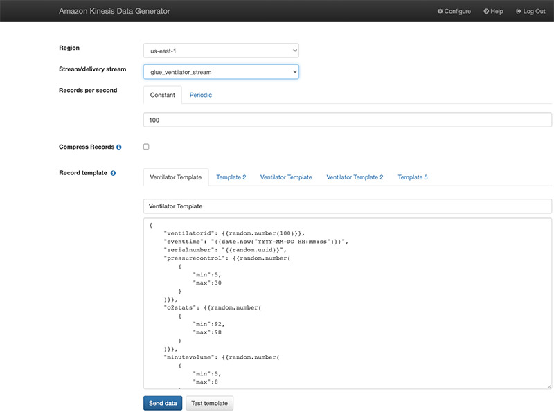
Using the Kinesis Data Generator
Alternatively, you can also use the Kinesis Data Generator with the ventilator template available on the GitHub repo. The following screenshot shows the template on the KDG console.

We start pushing the data after we create our AWS Glue streaming job.
Defining the schema
We need to specify a schema for our streaming data, which we can do one of two ways:
- Retrieve a small batch of the data (before starting your streaming job) from the streaming source, infer the schema in batch mode, and use the extracted schema for your streaming job
- Use the AWS Glue Data Catalog to manually create a table
For this post, we use the AWS Glue Data Catalog to create a ventilator schema.
- On the AWS Glue console, choose Data Catalog.
- Choose Tables.
- From the Add Table drop-down menu, choose Add table manually.
- For the table name, enter
ventilators_table.
- Create a database with the name
ventilatordb.
- Choose Kinesis as the type of source.
- Enter the name of the stream and
https://kinesis.<aws-region>.amazonaws.com.
- For the classification, choose JSON.
- Define the schema according to the following table.
| Column name |
Data type |
ventilatorid |
int |
eventtime |
string |
serialnumber |
string |
pressurecontrol |
int |
o2stats |
int |
minutevolume |
int |
manufacturer |
string |
- Choose Finish.
Creating an AWS Glue streaming job to hydrate a data lake on Amazon S3
With the streaming source and schema prepared, we’re now ready to create our AWS Glue streaming jobs. We first create a job to ingest data from the streaming source using AWS Glue DataFrame APIs.
- On the AWS Glue console, under ETL, choose Jobs.
- Choose Add job.
- For Name, enter a UTF-8 String with no more than 255 characters.
- For IAM role¸ specify a role that is used for authorization to resources used to run the job and access data stores. Because streaming jobs require connecting to sources and sinks, you need to make sure that the AWS Identity and Access Management (IAM) role has permissions to read from Kinesis Data Stream, write to Amazon S3 and read, write to Amazon DynamoDB. Refer to Managing Access Permissions for AWS Glue Resources for details.
- For Type, choose Spark Streaming.
- For Glue Version, choose Spark 2.4, Python 3.
- For This job runs, select A new script authored by you.
You can have AWS Glue generate the streaming ETL code for you, but for this post, we author one from scratch.
- For Script file name, enter
GlueStreaming-S3.
- For S3 path where script is stored, enter your S3 path.

- For Job bookmark, choose Disable.
For this post, we use the checkpointing mechanism of AWS Glue to keep track of the data read instead of a job bookmark.
- For Monitoring options, select Job metrics and Continuous logging.
- For Log filtering, select Standard filter and Spark UI.
- For Amazon S3 prefix for Spark event logs, enter the S3 path for the event logs.

- For Job parameters, enter the following key-values:
- –output path – The S3 path where the final aggregations are persisted
- –aws_region – The Region where you run the job

- Skip the connections part and choose Save and edit the script.
Streaming ETL to an Amazon S3 sink
We use the AWS Glue DynamicFrameReader class’s from_catalog method to read the streaming data. We specify the table name that has been associated with the data stream as the source of data (see the section Defining the schema). We add additional_options to indicate the starting position to read from in Kinesis Data Streams. TRIM_HORIZON allows us to start reading from the oldest record in the shard.
# Read from Kinesis Data Stream
sourceData = glueContext.create_data_frame.from_catalog( \
    database = "ventilatordb", \
    table_name = "ventilatortable", \
    transformation_ctx = "datasource0", \
    additional_options = {"startingPosition": "TRIM_HORIZON", "inferSchema": "true"})
In the preceding code, sourceData represents a streaming DataFrame. We use the foreachBatch API to invoke a function (processBatch) that processes the data represented by this streaming DataFrame. The processBatch function receives a static DataFrame, which holds streaming data for a window size of 100s (default). It creates a DynamicFrame from the static DataFrame and writes out partitioned data to Amazon S3. See the following code:
glueContext.forEachBatch(frame = sourceData, batch_function = processBatch, options = {"windowSize": "100 seconds", "checkpoint_locationation": checkpoint_location})
To transform the DynamicFrame to fix the data type for eventtime (from string to timestamp) and write the ventilator metrics to Amazon S3 in Parquet format, enter the following code:
def processBatch(data_frame, batchId):
    now = datetime.datetime.now()
    year = now.year
    month = now.month
    day = now.day
    hour = now.hour
    minute = now.minute
    if (data_frame.count() > 0):
        dynamic_frame = DynamicFrame.fromDF(data_frame, glueContext, "from_data_frame")
        apply_mapping = ApplyMapping.apply(frame = dynamic_frame, mappings = [ \
            ("ventilatorid", "long", "ventilatorid", "long"), \
            ("eventtime", "string", "eventtime", "timestamp"), \
            ("serialnumber", "string", "serialnumber", "string"), \
            ("pressurecontrol", "long", "pressurecontrol", "long"), \
            ("o2stats", "long", "o2stats", "long"), \
            ("minutevolume", "long", "minutevolume", "long"), \
            ("manufacturer", "string", "manufacturer", "string")],\
            transformation_ctx = "apply_mapping")

        dynamic_frame.printSchema()

        # Write to S3 Sink
        s3path = s3_target + "/ingest_year=" + "{:0>4}".format(str(year)) + "/ingest_month=" + "{:0>2}".format(str(month)) + "/ingest_day=" + "{:0>2}".format(str(day)) + "/ingest_hour=" + "{:0>2}".format(str(hour)) + "/"
        s3sink = glueContext.write_dynamic_frame.from_options(frame = apply_mapping, connection_type = "s3", connection_options = {"path": s3path}, format = "parquet", transformation_ctx = "s3sink")
Putting it all together
In the Glue ETL code editor, enter the following code, then save and run the job:
import sys
import datetime
import boto3
import base64
from pyspark.sql import DataFrame, Row
from pyspark.context import SparkContext
from pyspark.sql.types import *
from pyspark.sql.functions import *
from awsglue.transforms import *
from awsglue.utils import getResolvedOptions
from awsglue.context import GlueContext
from awsglue.job import Job
from awsglue import DynamicFrame

args = getResolvedOptions(sys.argv, \
                            ['JOB_NAME', \
                            'aws_region', \
                            'output_path'])

sc = SparkContext()
glueContext = GlueContext(sc)
spark = glueContext.spark_session
job = Job(glueContext)
job.init(args['JOB_NAME'], args)

# S3 sink locations
aws_region = args['aws_region']
output_path = args['output_path']

s3_target = output_path + "ventilator_metrics"
checkpoint_location = output_path + "cp/"
temp_path = output_path + "temp/"


def processBatch(data_frame, batchId):
    now = datetime.datetime.now()
    year = now.year
    month = now.month
    day = now.day
    hour = now.hour
    minute = now.minute
    if (data_frame.count() > 0):
        dynamic_frame = DynamicFrame.fromDF(data_frame, glueContext, "from_data_frame")
        apply_mapping = ApplyMapping.apply(frame = dynamic_frame, mappings = [ \
            ("ventilatorid", "long", "ventilatorid", "long"), \
            ("eventtime", "string", "eventtime", "timestamp"), \
            ("serialnumber", "string", "serialnumber", "string"), \
            ("pressurecontrol", "long", "pressurecontrol", "long"), \
            ("o2stats", "long", "o2stats", "long"), \
            ("minutevolume", "long", "minutevolume", "long"), \
            ("manufacturer", "string", "manufacturer", "string")],\
            transformation_ctx = "apply_mapping")

        dynamic_frame.printSchema()

        # Write to S3 Sink
        s3path = s3_target + "/ingest_year=" + "{:0>4}".format(str(year)) + "/ingest_month=" + "{:0>2}".format(str(month)) + "/ingest_day=" + "{:0>2}".format(str(day)) + "/ingest_hour=" + "{:0>2}".format(str(hour)) + "/"
        s3sink = glueContext.write_dynamic_frame.from_options(frame = apply_mapping, connection_type = "s3", connection_options = {"path": s3path}, format = "parquet", transformation_ctx = "s3sink")

# Read from Kinesis Data Stream
sourceData = glueContext.create_data_frame.from_catalog( \
    database = "ventilatordb", \
    table_name = "ventilatortable", \
    transformation_ctx = "datasource0", \
    additional_options = {"startingPosition": "TRIM_HORIZON", "inferSchema": "true"})

sourceData.printSchema()

glueContext.forEachBatch(frame = sourceData, batch_function = processBatch, options = {"windowSize": "100 seconds", "checkpoint_locationation": checkpoint_location})
job.commit()
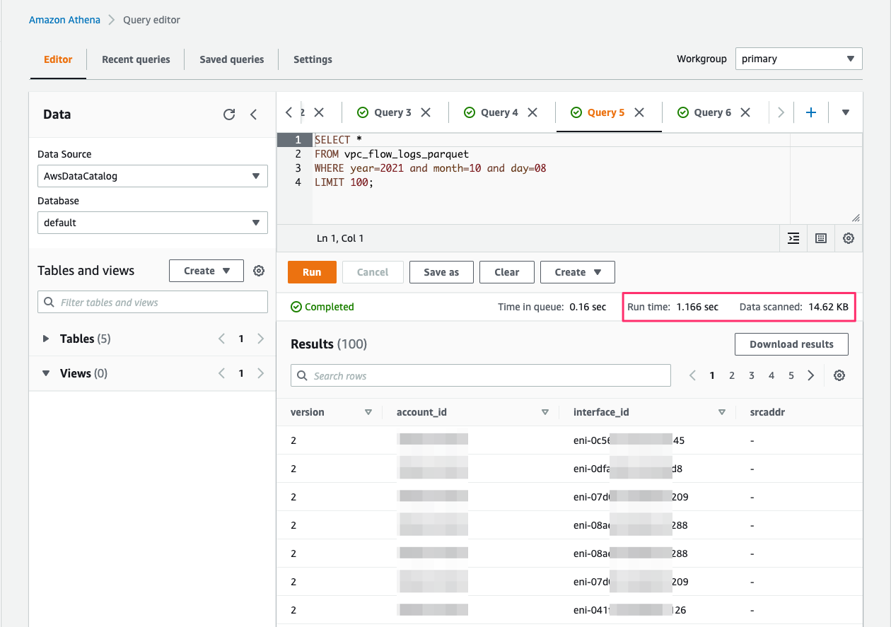
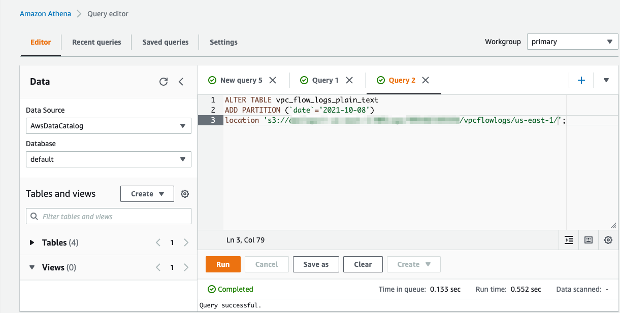
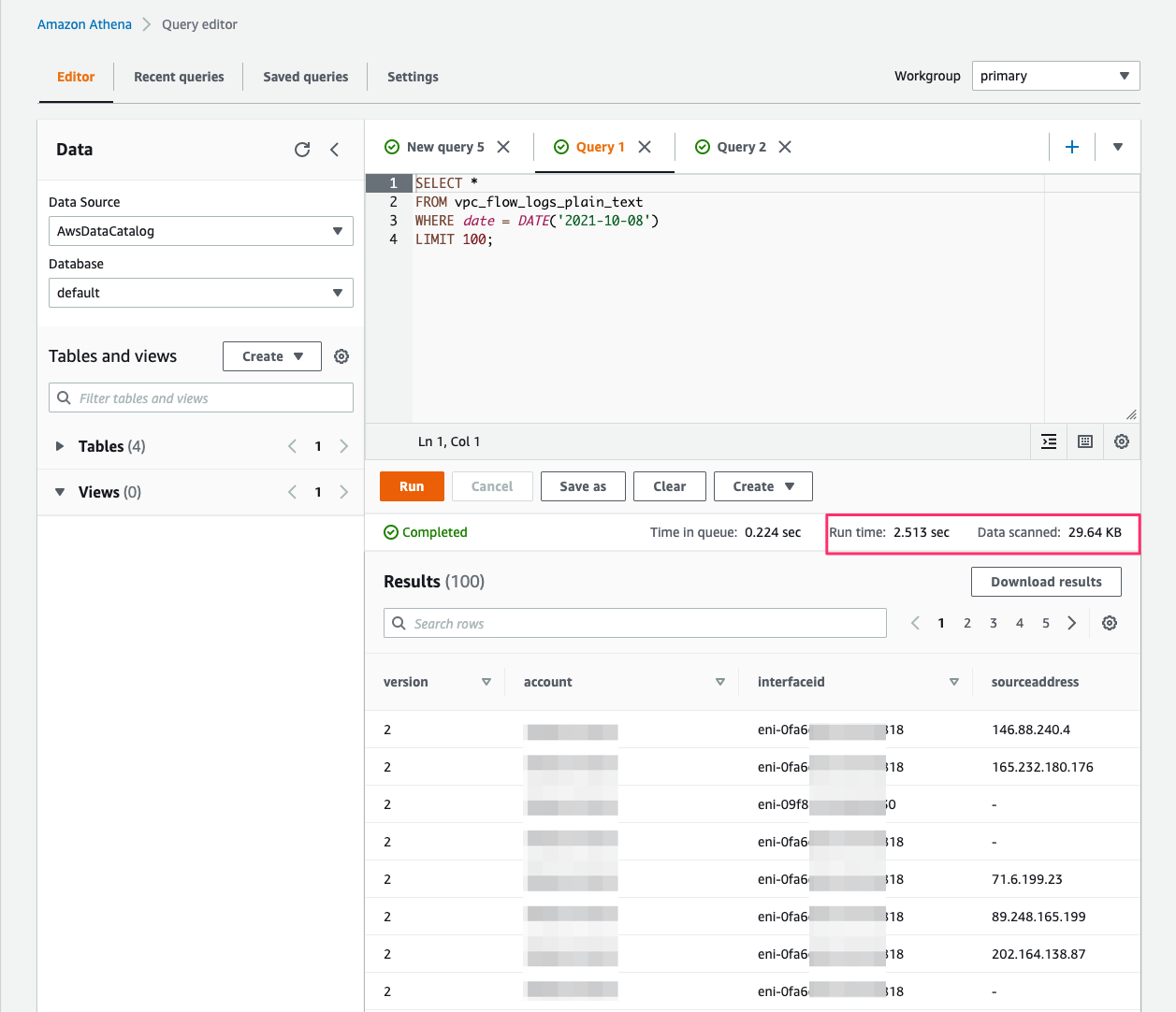
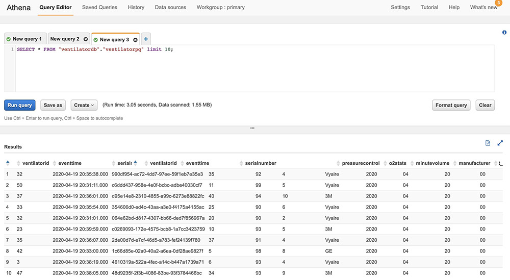
Querying with Athena
When the processed streaming data is written in Parquet format to Amazon S3, we can run queries on Athena. Run the AWS Glue crawler on the Amazon S3 location where the streaming data is written out. The following screenshot shows our query results.

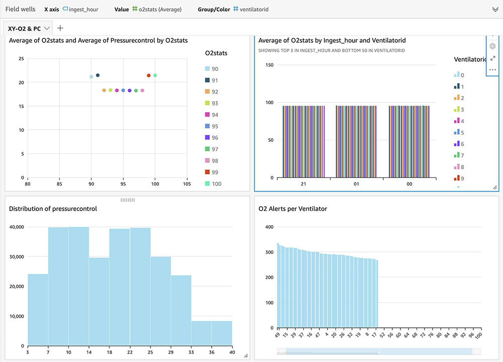
For instructions on building visual dashboards with the streaming data in Amazon S3, see Quick Start: Create an Analysis with a Single Visual Using Sample Data. The following dashboards show distribution of metrics, averages, and alerts based on anomalies on an hourly basis, but you can create more advanced dashboards with much granular (minute) intervals.

Streaming ETL to a DynamoDB sink
For the second use case, we transform the streaming data as it arrives without micro-batching and persist the data to a DynamoDB table. Scripts to create DynamoDB tables are available in the GitHub repo. We use Apache Spark’s Structured Streaming API to read ventilator-generated data from the data stream, join it with reference data for normal metrics range in a DynamoDB table, compute the status based on the deviation from normal metric values, and write the processed data to a DynamoDB table. See the following code:
import sys
import datetime
import base64
import decimal
import boto3
from pyspark.sql import DataFrame, Row
from pyspark.context import SparkContext
from pyspark.sql.types import *
from pyspark.sql.functions import *
from awsglue.transforms import *
from awsglue.utils import getResolvedOptions
from awsglue.context import GlueContext
from awsglue.job import Job
from awsglue import DynamicFrame

args = getResolvedOptions(sys.argv, \
                            ['JOB_NAME', \
                            'aws_region', \
                            'checkpoint_location', \
                            'dynamodb_sink_table', \
                            'dynamodb_static_table'])

sc = SparkContext()
glueContext = GlueContext(sc)
spark = glueContext.spark_session
job = Job(glueContext)
job.init(args['JOB_NAME'], args)

# Read parameters
checkpoint_location = args['checkpoint_location']
aws_region = args['aws_region']

# DynamoDB config
dynamodb_sink_table = args['dynamodb_sink_table']
dynamodb_static_table = args['dynamodb_static_table']

def write_to_dynamodb(row):
    '''
    Add row to DynamoDB.
    '''
    dynamodb = boto3.resource('dynamodb', region_name=aws_region)
    start = str(row['window'].start)
    end = str(row['window'].end)
    dynamodb.Table(dynamodb_sink_table).put_item(
      Item = { 'ventilatorid': row['ventilatorid'], \
                'status': str(row['status']), \
                'start': start, \
                'end': end, \
                'avg_o2stats': decimal.Decimal(str(row['avg_o2stats'])), \
                'avg_pressurecontrol': decimal.Decimal(str(row['avg_pressurecontrol'])), \
                'avg_minutevolume': decimal.Decimal(str(row['avg_minutevolume']))})

dynamodb_dynamic_frame = glueContext.create_dynamic_frame.from_options( \
    "dynamodb", \
    connection_options={
    "dynamodb.input.tableName": dynamodb_static_table,
    "dynamodb.throughput.read.percent": "1.5"
  }
)

dynamodb_lookup_df = dynamodb_dynamic_frame.toDF().cache()

# Read from Kinesis Data Stream
streaming_data = spark.readStream \
                    .format("kinesis") \
                    .option("streamName","glue_ventilator_stream") \
                    .option("endpointUrl", "https://kinesis.us-east-1.amazonaws.com") \
                    .option("startingPosition", "TRIM_HORIZON") \
                    .load()

# Retrieve Sensor columns and do a simple projection
ventilator_fields = streaming_data \
    .select(from_json(col("data") \
    .cast("string"),glueContext.get_catalog_schema_as_spark_schema("ventilatordb","ventilators_table")) \
    .alias("ventilatordata")) \
    .select("ventilatordata.*") \
    .withColumn("event_time", to_timestamp(col('eventtime'), "yyyy-MM-dd HH:mm:ss")) \
    .withColumn("ts", to_timestamp(current_timestamp(), "yyyy-MM-dd HH:mm:ss"))

# Stream static join, ETL to augment with status
ventilator_joined_df = ventilator_fields.join(dynamodb_lookup_df, "ventilatorid") \
    .withColumn('status', when( \
    ((ventilator_fields.o2stats < dynamodb_lookup_df.o2_stats_min) | \
    (ventilator_fields.o2stats > dynamodb_lookup_df.o2_stats_max)) & \
    ((ventilator_fields.pressurecontrol < dynamodb_lookup_df.pressure_control_min) | \
    (ventilator_fields.pressurecontrol > dynamodb_lookup_df.pressure_control_max)) & \
    ((ventilator_fields.minutevolume < dynamodb_lookup_df.minute_volume_min) | \
    (ventilator_fields.minutevolume > dynamodb_lookup_df.minute_volume_max)), "RED") \
    .when( \
    ((ventilator_fields.o2stats >= dynamodb_lookup_df.o2_stats_min) |
    (ventilator_fields.o2stats <= dynamodb_lookup_df.o2_stats_max)) & \
    ((ventilator_fields.pressurecontrol >= dynamodb_lookup_df.pressure_control_min) | \
    (ventilator_fields.pressurecontrol <= dynamodb_lookup_df.pressure_control_max)) & \
    ((ventilator_fields.minutevolume >= dynamodb_lookup_df.minute_volume_min) | \
    (ventilator_fields.minutevolume <= dynamodb_lookup_df.minute_volume_max)), "GREEN") \
    .otherwise("ORANGE"))

ventilator_joined_df.printSchema()

# Drop the normal metric values
ventilator_transformed_df = ventilator_joined_df \
                            .drop('eventtime', 'o2_stats_min', 'o2_stats_max', \
                            'pressure_control_min', 'pressure_control_max', \
                            'minute_volume_min', 'minute_volume_max')

ventilator_transformed_df.printSchema()

ventilators_df = ventilator_transformed_df \
    .groupBy(window(col('ts'), '10 minute', '5 minute'), \
    ventilator_transformed_df.status, ventilator_transformed_df.ventilatorid) \
    .agg( \
    avg(col('o2stats')).alias('avg_o2stats'), \
    avg(col('pressurecontrol')).alias('avg_pressurecontrol'), \
    avg(col('minutevolume')).alias('avg_minutevolume') \
    )

ventilators_df.printSchema()

# Write to DynamoDB sink
ventilator_query = ventilators_df \
    .writeStream \
    .foreach(write_to_dynamodb) \
    .outputMode("update") \
    .option("checkpointLocation", checkpoint_location) \
    .start()

ventilator_query.awaitTermination()

job.commit()
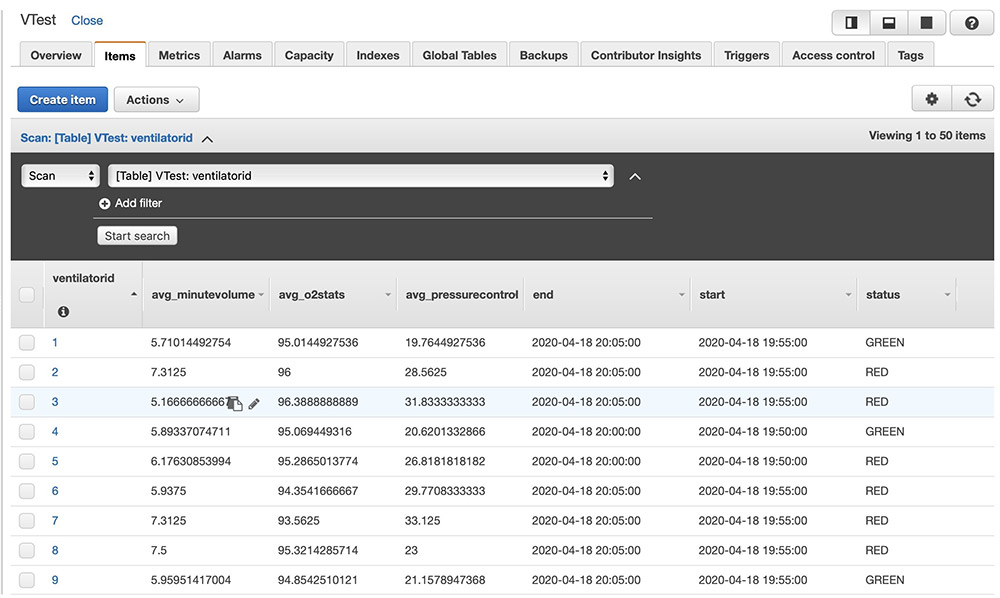
After the above code is run, ventilator metric aggregations get persisted in the Amazon DynamoDB table as follows. You can build custom user interface applications with the data in Amazon DynamoDB to create dashboards.

Conclusion
Streaming applications have become a core component of data lake architectures. With AWS Glue streaming, you can create serverless ETL jobs that run continuously, consuming data from streaming services like Kinesis Data Streams and Amazon MSK. You can load the results of streaming processing into an Amazon S3-based data lake, JDBC data stores, or arbitrary sinks using the Structured Streaming API.
For more information about streaming AWS Glue ETL jobs, see the following:
We encourage you to build a serverless streaming application using AWS Glue streaming ETL and share your experience with us. If you have any questions or suggestions, share them in the comments.
About the Author
 Radhika Ravirala is a specialist solutions architect at Amazon Web Services,
 where she helps customers craft distributed analytics applications on the AWS platform. Prior to her cloud journey, she worked as a software engineer and designer for technology companies in Silicon Valley.

 Radhika Ravirala is the Principal Product Manager at AWS.
 Matthew Liem is the Senior Solution Architecture Manager at AWS.