Post Syndicated from Sachin Thakkar original https://aws.amazon.com/blogs/big-data/backtest-trading-strategies-with-amazon-kinesis-data-streams-long-term-retention-and-amazon-sagemaker/
Real-time insight is critical when it comes to building trading strategies. Any delay in data insight can cost lot of money to the traders. Often, you need to look at historical market trends to predict future trading pattern and make the right bid. More the historical data you analyze, better trading prediction you get. Back tracking streaming data can be tricky as it requires sophisticated storage and analysis mechanisms.
Amazon Kinesis Data Streams allows our customer to store streaming data for up to one year. Amazon Kinesis Data Streams Long Term Retention (LTR) of streaming data enables to use the same platform for both real-time and older data retained in Amazon Kinesis Data Streams. For example, one can train machine learning algorithms for financial trading, marketing personalization, and recommendation models without moving the data into a different data store or writing a new application. Customers can also satisfy certain data retention regulations, including under HIPAA and FedRAMP, using long term retention. This thus simplifies the data ingestion architecture for our trading use case we will discuss in this post.
In the post Building algorithmic trading strategies with Amazon SageMaker, we demonstrated how to backtest trading strategies with Amazon SageMaker with historical stock price data stored in Amazon Simple Storage Service (Amazon S3). In this post, we expand this solution for streaming data and describe how to use Amazon Kinesis.
In addition, we want to use Amazon SageMaker automatic tuning to find the optimal configuration for a moving average crossover strategy. In this strategy, two moving averages for a slow and a fast time period are calculated, and a trade is executed when a crossover happens. If the fast moving average crosses above the slow moving average, the strategy places a long trade, otherwise the strategy goes short. We find the optimal period length for these moving averages by running multiple backtests with different lengths over a historical dataset.
Finally, we run the optimal configuration for this moving average crossover strategy over a different test dataset and analyze the performance results. If the performance measured in profit and loss (P&L) is positive for the test period, we can consider this trading strategy for a forward test.
To show you how easy and quick it is to get started on AWS, we provide a one-click deployment for an extensible trading backtesting solution that uses Kinesis long-term retention for streaming data.
Solution overview
We use Kinesis Data Streams to store real-time streaming as well as historical market data. We use Jupyter notebooks as our central interface for exploring and backtesting new trading strategies. SageMaker allows you to set up Jupyter notebooks and integrate them with AWS CodeCommit to store different versions of strategies and share them with other team members.
We use Amazon S3 to store model artifacts and backtesting results.
For our trading strategies, we create Docker containers that contain the required libraries for backtesting and the strategy itself. These containers follow the SageMaker Docker container structure in order to run them inside of SageMaker. For more information about the structure of SageMaker containers, see Using the SageMaker Training and Inference Toolkits.
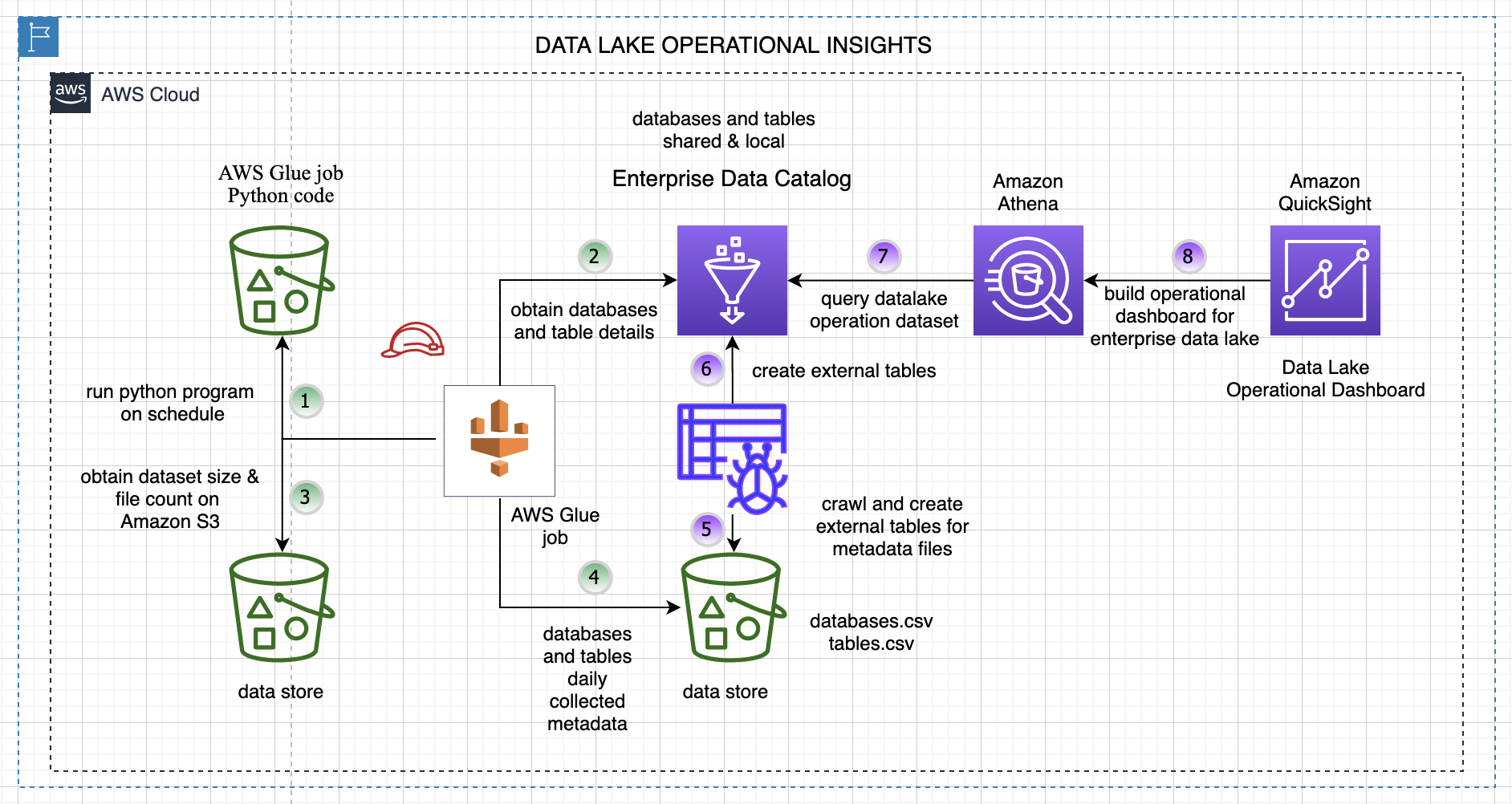
The following diagram illustrates this architecture.

We run the data preparation step from a SageMaker notebook. This copies the historical market data to the S3 bucket.
We use AWS Data Migration Service (AWS DMS) to load the market data to the data stream. The
SageMaker notebook connects with Kinesis Data Streams and runs the trading strategy algorithm via a SageMaker training job. The algorithm uses part of the data for training to find the optimal strategy configuration.
Finally, we run the trading strategy using the previously determined configuration on a test dataset.
Prerequisites
Before getting started, we set up our resources. In this post, we use the us-east-2 Region as an example.
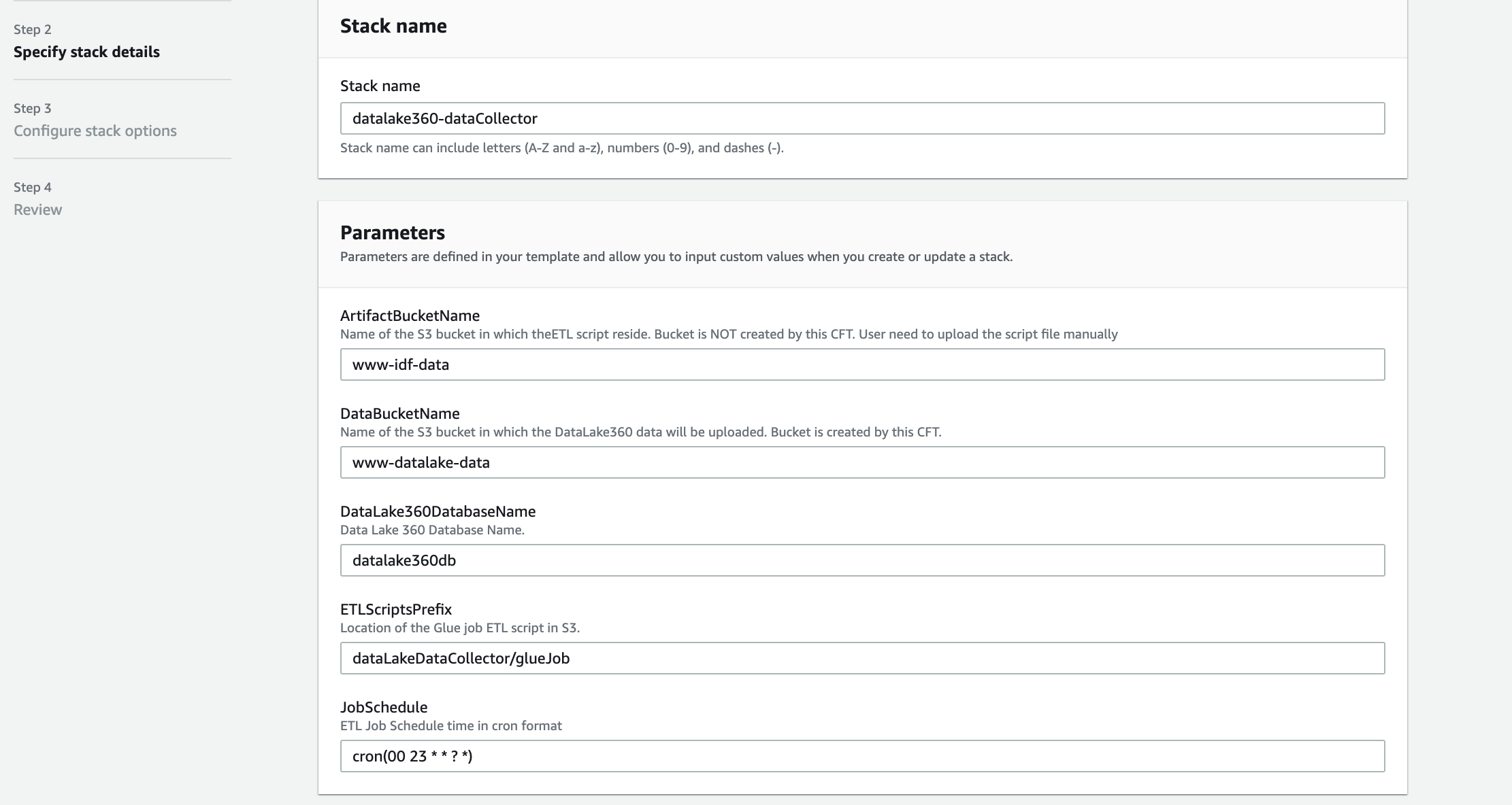
- Deploy the AWS resources using the provided AWS CloudFormation template.

- For Stack name, enter a name for your stack.
- Provide an existing S3 bucket name to store the historical market data.
The data is loaded in Kinesis Data Streams from this S3 bucket. Your bucket needs to be in same Region where your stack is set up.

- Accept all the defaults and choose Next.
- Acknowledge that AWS CloudFormation might create AWS Identity and Access Management (IAM) resources with custom names.
- Choose Create stack.

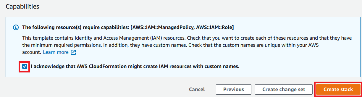
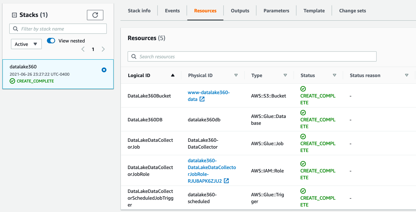
This creates all the required resources.
Data load to Kinesis Data Streams
To perform the data load, complete the following steps:
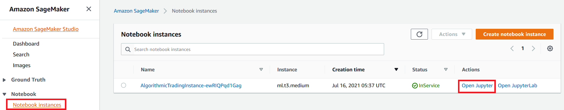
- On the SageMaker console, under Notebook in the navigation pane, choose Notebook instances.
- Locate the notebook instance
AlgorithmicTradingInstance-*. - Choose Open Jupyter for this instance.

- Go to the
algorithmic-trading->4_Kinesisfolder and choose Strategy_Kinesis_EMA_HPO.pynb.
You now run the data preparation step in the notebook.
- Load the dataset.


Specify the existing bucket where test data is stored. Make sure that the test bucket is in the same Region where you set up the stack.
- Run all the steps in the notebook until Step 2 Data Preparation.
- On the AWS DMS console, choose Database migration tasks.
- Select the AWS DMS task
dmsreplicationtask-*. - On the Actions menu, choose Restart/Resume.
This starts the data load from the S3 bucket to the data stream.

Wait until the replication task shows the status Load complete.

- Continue the steps in the Jupyter notebook.

Read data from Kinesis long-term retention
We read daily open, high, low, close price, and volume data from the stream’s long-term retention with the AWS SDK for Python (Boto3).
Although we don’t use enhanced fan-out (EFO) in this post, it may be advisable to do so an existing application is already reading from the stream. That way this backtesting app doesn’t interfere with the existing application.

You can visualize your data, as shown in the following screenshot.

Define your trading strategy
In this step, we define our moving average crossover trading strategy.

Build a Docker image
We build our backtesting job as a Docker image and push it to Amazon ECR.

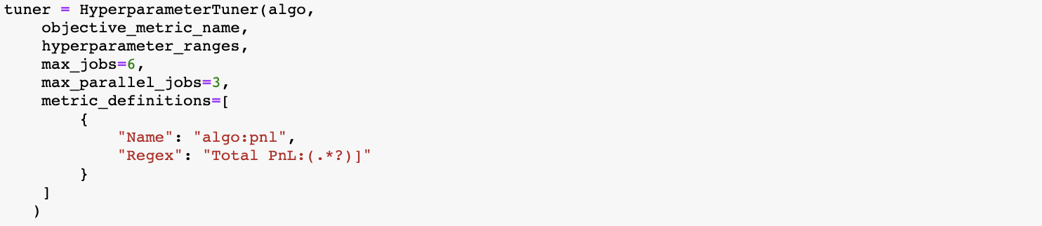
Hyperparameter optimization with SageMaker on training data
For the moving average crossover trading strategy, we want to find the optimal fast period and slow period of this strategy, and we provide a range of days to search for.

We use profit and loss (P&L) of the strategy as the metric to find optimized hyperparameters.
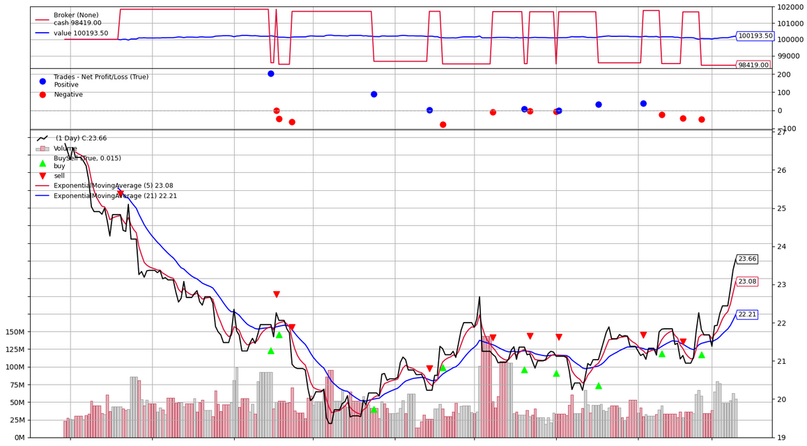
You can see the tuning job recommended a value of 7 and 21 days for the fast and slow period for this trading strategy given the training dataset.

Run the strategy with optimal hyperparameters on test data
We now run this strategy with optimal hyperparameters on the test data.


When the job is complete, the performance results are stored in Amazon S3, and you can review the performance metrics in a chart and analyze the buy and sell orders for your strategy.
Conclusion
In this post, we described how to use the Kinesis Data Streams long-term retention feature to store the historical stock price data and how to use streaming data for backtesting of a trading strategy with SageMaker.
Long-term retention of streaming data enables you to use the same platform for both real-time and older data retained in Kinesis Data Streams. This allows you to use this data stream for financial use cases like backtesting or for machine learning without moving the data into a different data store or writing a new application. You can also satisfy certain data retention regulations, including under HIPAA and FedRAMP, using long-term retention. For more information, see Amazon Kinesis Data Streams enables data stream retention up to one year.
Risk disclaimer
This post is for educational purposes only and past trading performance does not guarantee future performance.
About the Authors
 Sachin Thakkar is a Senior Solutions Architect at Amazon Web Services, working with a leading Global System Integrator (GSI). He brings over 22 years of experience as an IT Architect and as Technology Consultant for large institutions. His focus area is on Data & Analytics. Sachin provides architectural guidance and supports the GSI partner in building strategic industry solutions on AWS
 Amogh Gaikwad is a Solutions Developer in the Prototyping Team. He specializes in machine learning and analytics and has extensive experience developing ML models in real-world environments and integrating AI/ML and other AWS services into large-scale production applications. Before joining Amazon, he worked as a software developer, developing enterprise applications focusing on Enterprise Resource Planning (ERP) and Supply Chain Management (SCM). Amogh has received his master’s in Computer Science specializing in Big Data Analytics and Machine Learning.
 Dhiraj Thakur is a Solutions Architect with Amazon Web Services. He works with AWS customers and partners to provide guidance on enterprise cloud adoption, migration and strategy. He is passionate about technology and enjoys building and experimenting in Analytics and AI/ML space.
 Oliver Steffmann is an Enterprise Solutions Architect at AWS based in New York. He brings over 18 years of experience as IT Architect, Software Development Manager, and as Management Consultant for international financial institutions. During his time as a consultant, he leveraged his extensive knowledge of Big Data, Machine Learning and cloud technologies to help his customers get their digital transformation off the ground. Before that he was the head of municipal trading technology at a tier-one investment bank in New York and started his career in his own startup in Germany.