Post Syndicated from Diego Garcia Garcia original https://aws.amazon.com/blogs/big-data/stream-real-time-data-into-apache-iceberg-tables-in-amazon-s3-using-amazon-data-firehose/
As businesses generate more data from a variety of sources, they need systems to effectively manage that data and use it for business outcomes—such as providing better customer experiences or reducing costs. We see these trends across many industries—online media and gaming companies providing recommendations and customized advertising, factories monitoring equipment for maintenance and failures, theme parks providing wait times for popular attractions, and many others.
To build such applications, engineering teams are increasingly adopting two trends. First, they’re replacing batch data processing pipelines with real-time streaming, so applications can derive insight and take action within seconds instead of waiting for daily or hourly batch exchange, transform, and load (ETL) jobs. Second, because traditional data warehousing approaches are unable to keep up with the volume, velocity, and variety of data, engineering teams are building data lakes and adopting open data formats such as Parquet and Apache Iceberg to store their data. Iceberg brings the reliability and simplicity of SQL tables to Amazon Simple Storage Service (Amazon S3) data lakes. By using Iceberg for storage, engineers can build applications using different analytics and machine learning frameworks such as Apache Spark, Apache Flink, Presto, Hive, or Impala, or AWS services such as Amazon SageMaker, Amazon Athena, AWS Glue, Amazon EMR, Amazon Managed Service for Apache Flink, or Amazon Redshift.
Iceberg is popular because first, it’s widely supported by different open-source frameworks and vendors. Second, it allows customers to read and write data concurrently using different frameworks. For example, you can write some records using a batch ETL Spark job and other data from a Flink application at the same time and into the same table. Third, it allows scenarios such as time travel and rollback, so you can run SQL queries on a point-in-time snapshot of your data, or rollback data to a previously known good version. Fourth, it supports schema evolution, so when your applications evolve, you can add new columns to your tables without having to rewrite data or change existing applications. To learn more, see Apache Iceberg.
In this post, we discuss how you can send real-time data streams into Iceberg tables on Amazon S3 by using Amazon Data Firehose. Amazon Data Firehose simplifies the process of streaming data by allowing users to configure a delivery stream, select a data source, and set Iceberg tables as the destination. Once set up, the Firehose stream is ready to deliver data. Firehose is integrated with over 20 AWS services, so you can deliver real-time data from Amazon Kinesis Data Streams, Amazon Managed Streaming for Apache Kafka, Amazon CloudWatch Logs, AWS Internet of Things (AWS IoT), AWS WAF, Amazon Network Firewall Logs, or from your custom applications (by invoking the Firehose API) into Iceberg tables. It’s cost effective because Firehose is serverless, you only pay for the data sent and written to your Iceberg tables. You don’t have to provision anything or pay anything when your streams are idle during nights, weekends, or other non-use hours.
Firehose also simplifies setting up and running advanced scenarios. For example, if you want to route data to different Iceberg tables to have data isolation or better query performance, you can set up a stream to automatically route records into different tables based on what’s in your incoming data and distribute records from a single stream into dozens of Iceberg tables. Firehose automatically scales—so you don’t have to plan for how much data goes into which table—and has built-in mechanisms to handle delivery failures and guarantee exactly once delivery. Firehose supports updating and deleting records in a table based on the incoming data stream, so you can support scenarios such as GDPR and right-to-forget regulations. Because Firehose is fully compatible with Iceberg, you can write data using it and simultaneously use other applications to read and write to the same tables. Firehose integrates with the AWS Glue Data Catalog, so you can use features in AWS Glue such as managed compaction for Iceberg tables.
In the following sections, you’ll learn how to set up Firehose to deliver real-time streams into Iceberg tables to address four different scenarios:
- Deliver data from a stream into a single Iceberg table and insert all incoming records.
- Deliver data from a stream into a single Iceberg table and perform record inserts, updates, and deletes.
- Route records to different tables based on the content of the incoming data by specifying a JSON Query expression.
- Route records to different tables based on the content of the incoming data by using a Lambda function.
You will also learn how to query the data you have delivered to Iceberg tables using a standard SQL query in Amazon Athena. All of the AWS services used in these examples are serverless, so you don’t have to provision and manage any infrastructure.
Solution overview
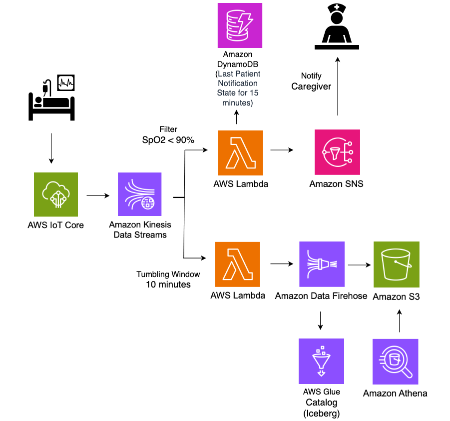
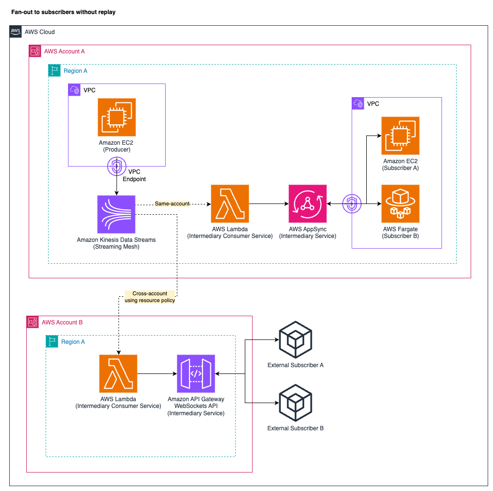
The following diagram illustrates the architecture.

In our examples, we use Kinesis Data Generator, a sample application to generate and publish data streams to Firehose. You can also set up Firehose to use other data sources for your real-time streams. We set up Firehose to deliver the stream into Iceberg tables in the Data Catalog.
Walkthrough
This post includes an AWS CloudFormation template for a quick setup. You can review and customize it to suit your needs. The template performs the following operations:
- Creates a Data Catalog database for the destination Iceberg tables
- Creates four tables in the AWS Glue database that are configured to use the Apache Iceberg format
- Specifies the S3 bucket locations for the destination tables
- Creates a Lambda function (optional)
- Sets up an AWS Identity and Access Management (IAM) role for Firehose
- Creates resources for Kinesis Data Generator
Prerequisites
For this walkthrough, you should have the following prerequisites:
- An AWS account. If you don’t have an account, you can create one.
Deploy the solution
The first step is to deploy the required resources into your AWS environment by using a CloudFormation template.
- Sign in to the AWS Management Console for CloudFormation.
- Choose Launch Stack.

- Choose Next.
- Leave the stack name as Firehose-Iceberg-Stack, and in the parameters, enter the username and password that you want to use for accessing Kinesis Data Generator.

- Go to the bottom of the page and select I acknowledge that AWS CloudFormation might create IAM resources and choose Next.

- Review the deployment and choose Submit.

The stack can take 5–10 minutes to complete, after which you can view the deployed stack on the CloudFormation console. The following figure shows the deployed Firehose-Iceberg-stack details.

Before you set up Firehose to deliver streams, you must create the destination tables in the Data Catalog. For the examples discussed here, we use the CloudFormation template to automatically create the tables used in the examples. For your custom applications, you can create your tables using CloudFormation, or by using DDL commands in Athena or Glue. The following is the DDL command for creating a table used in our example:
CREATE TABLE firehose_iceberg_db.firehose_events_1 (
type struct<device: string, event: string, action: string>,
customer_id string,
event_timestamp timestamp,
region string)
LOCATION 's3://firehose-demo-iceberg-<account_id>-<region>/iceberg/events_1'
TBLPROPERTIES (
'table_type'='iceberg',
'write_compression'='zstd'
);
Also note that the four tables that we use in the examples have the same schema, but you can have tables with different schemas in your application.
Use case 1: Deliver data from a stream into a single Iceberg table and insert all incoming records
Now that you have set up the source for your data stream and the destination tables, you’re ready to set up Firehose to deliver streams into the Iceberg tables.
Create a Firehose stream:
- Go to the Data Firehose console and choose Create Firehose stream.

- Select Direct PUT as the Source and Apache Iceberg Tables as the Destination.
This example uses Direct PUT as the source, but the same steps can be applied for other Firehose sources such as Kinesis Data Streams, and Amazon MSK.

- For the Firehose stream name, enter
firehose-iceberg-events-1.

- In Destination settings, enable Inline parsing for routing information. Because all records from the stream are inserted into a single destination table, you specify a destination database and table. By default, Firehose inserts all incoming records into the specified destination table.
- Database expression: “
firehose_iceberg_db”
- Table expression: “
firehose_events_1”
Include double quotation marks to use the literal value for the database and table name. If you do not use double quotations marks, Firehose assumes that this is a JSON Query expression and will attempt to parse the expression when processing your stream and fail.

- Go to Buffer hints and reduce the Buffer size to 1 MiB and the Buffer interval to 60 You can fine tune these settings for your application.

- For Backup settings:
- Select the S3 bucket created by the CloudFormation template. It has the following structure:
s3://firehose-demo-iceberg-<account_id>-<region>
- For error output prefix enter:
error/events-1/

- In Advanced settings, enable CloudWatch error logging, and in Existing IAM roles, select the role that starts with Firehose-Iceberg-Stack-FirehoseIamRole-*, created by the CloudFormation template.
- Choose Create Firehose stream.

Generate streaming data:
Use Kinesis Data Generator to publish data records into your Firehose stream.
- Go to the CloudFormation stack, select the Nested stack for the generator, and choose Outputs.

- Choose the KinesisDataGenerator URL and enter the credentials that you defined when deploying the CloudFormation stack.

- Select the AWS Region where you deployed the CloudFormation stack and select your Firehose stream.

- For template, replace the values on the screen with the following:
{
"type": {
"device": "{{random.arrayElement(["mobile", "desktop", "tablet"])}}",
"event": "{{random.arrayElement(["firehose_events_1", "firehose_events_2"])}}",
"action": "update"
},
"customer_id": "{{random.number({ "min": 1, "max": 1500})}}",
"event_timestamp": "{{date.now("YYYY-MM-DDTHH:mm:ss.SSS")}}",
"region": "{{random.arrayElement(["pdx", "nyc"])}}"
}
- Before sending data, choose Test template to see an example payload.
- Choose Send data.

Querying with Athena:
You can query the data you’ve written to your Iceberg tables using different processing engines such as Apache Spark, Apache Flink, or Trino. In this example, we will show you how you can use Athena to query data that you’ve written to Iceberg tables.
- Go to the Athena console.
- Configure a Location of query result. You can use the same S3 bucket for this but add a suffix at the end.
s3://firehose-demo-iceberg-<account_id>-<region>/athena/

- In the query editor, in Tables and views, select the options button next to firehose_events_1 and select Preview Table.

You should be able to see data in the Apache Iceberg tables by using Athena.

With that, you ‘ve delivered data streams into an Apache Iceberg table using Firehose and run a SQL query against your data.
Now let’s explore the other scenarios. We will follow the same procedure as before for creating the Firehose stream and querying Iceberg tables with Amazon Athena.
Use case 2: Deliver data from a stream into a single Iceberg table and perform record inserts, updates, and deletes
One of the advantages of using Apache Iceberg is that it allows you to perform row-level operations such as updates and deletes on tables in a data lake. Firehose can be set up to automatically apply record update and delete operations in your Iceberg tables.
Things to know:
- When you apply an update or delete operation through Firehose, the data in Amazon S3 isn’t actually deleted. Instead, a marker record is written according to the Apache Iceberg format specification to indicate that the record is updated or deleted, so subsequent read and write operations get the latest record. If you want to purge (remove the underlying data from Amazon S3) the deleted records, you can use tools developed for purging records in Apache Iceberg.
- If you attempt to update a record using Firehose and the underlying record doesn’t already exist in the destination table, Firehose will insert the record as a new row.
Create a Firehose stream:
- Go to the Amazon Data Firehose console.
- Choose Create Firehose stream.
- For Source, select Direct PUT. For Destination select Apache Iceberg Tables.
- For the Firehose stream name, enter
firehose-iceberg-events-2.
- In the e, enable inline parsing for routing information and provide the required values as static values for Database expression and Table expression. Because you want to be able to update records, you also need to specify the Operation expression.
- Database expression: “
firehose_iceberg_db”
- Table expression: “
firehose_events_2”
- Operation expression: “
update”
Include double quotation marks to use the literal value for the database and table name. If you do not use double quotations marks, Firehose assumes that this is a JSON Query expression and will attempt to parse the expression when processing your stream and fail.

- Because you want to perform update and delete operations, you need to provide the columns in the destination table that will be used as unique keys to identify the record in the destination to be updated or deleted.
- For DestinationDatabaseName: “
firehose_iceberg_db“
- For DestinationTableName: “
firehose_events_2”
- In UniqueKeys, replace the existing value with: “
customer_id”

- Change the Buffer hints to
1 MiB and 60
- In Backup settings, select the same bucket from the stack, but enter the following in the error output prefix:
- In Advanced settings, enable CloudWatch Error logging and select the existing role of the stack and create the new Firehose stream.
Use Kinesis Data Generator to publish records into your Firehose stream. You might need to refresh the page or change regions so that it refreshes and shows the newly created delivery stream.
Don’t make any changes to the template and start sending data to the firehose-iceberg-events-2 stream.
Run the following query in Athena to see data in the firehose_events_2 table. Note that you can send updated records for the same unique key (same customer_id value) into your Firehose stream, and Firehose automatically applies record updates in the destination table. Thus, when you query data in Athena, you will see only one record for each unique value of customer_id, even if you have sent multiple updates into your stream.
SELECT customer_id, count(*)
FROM "firehose_iceberg_db"."firehose_events_2"
GROUP BY customer_id LIMIT 10;
Use case 3: Route records to different tables based on the content of the incoming data by specifying a JSON Query expression
Until now, you provided the routing and operation information as static values to perform operations on a single table. However, you can specify JSON Query expressions to define how Firehose should retrieve the destination database, destination table, and operation from your incoming data stream, and accordingly route the record and perform the corresponding operation. Based on your specification, Firehose automatically routes and delivers each record into the appropriate destination table and applies the corresponding operation.
Create a Firehose stream:
- Go back to the Amazon Data Firehose console.
- Choose Create Firehose Stream.
- For Source, select Direct PUT. For Destination, select Apache Iceberg Tables.
- For the Firehose stream name, enter
firehose-iceberg-events-3.

- In Destination settings, enable Inline parsing for routing information.
- For Database expression, provide the same value as before as a static string: “
firehose_iceberg_db”
- For Table expression, retrieve this value from the nested incoming record using JSON Query.
- For Operation expression, we will also retrieve this value from our nested record using JSON Query.
If you have the following incoming events with different event values, With the preceding JSON Query expressions, Firehose will parse and get “firehose_event_3” or “firehose_event_4” as the table names, and “update” as the intended operation from the incoming records.
{ "type": {   "device": "tablet",
"event": "firehose_events_3",   "action": "update" },
"customer_id": "112", "event_timestamp": "2024-10-02T15:46:52.901",
"region": "pdx"}
{ "type": {   "device": "tablet",
"event": "firehose_events_4",   "action": "update" },
"customer_id": "112", "event_timestamp": "2024-10-02T15:46:52.901",
"region": "pdx"}

- Because this is an update operation, you need to configure unique keys for each table. Also, because you want to deliver records to multiple Iceberg tables, you need to provide configurations for each of the two destination tables that records can be written to.

- Change the Buffer hints to 1 MiB and 60
- In Backup settings, select the same bucket from the stack, but in the error output prefix enter the following:
- In Advanced settings, select the existing IAM role created by the CloudFormation stack and create the new Firehose stream.
- In Kinesis Data Generator, refresh the page and select the newly created Firehose stream:
firehose-iceberg-events-3
If you query the firehose_events_3 and firehose_events_4 tables using Athena, you should find the data routed to right tables by Firehose using the routing information retrieved using JSON Query expressions.
Table below showing events with event “firehose_events_3”

The following figure shows Firehose Events Table 4.

Use Case 4: Route records to different tables based on the content of the incoming data by using a Lambda function
There might be scenarios where routing information isn’t readily available in the input record. You might want to parse and process incoming records or perform a lookup to determine where to deliver the record and whether to perform an update or delete operation. For such scenarios, you can use a Lambda function to generate the routing information and operation specification. Firehose automatically invokes your Lambda function for a batch of records (with a configurable batch size). You can process incoming records in your Lambda function and provide the routing information and operation in the output of the function. To learn more about how to process Firehose records using Lambda, see Transform source data in Amazon Data Firehose. After executing your Lambda function, Firehose looks for routing information and operations in the metadata fields (in the following format) provided by your Lambda function.
    "metadata":{
        "otfMetadata":{
            "destinationTableName":"firehose_iceberg_db",
            "destinationDatabaseName":"firehose_events_*",
            "operation":"insert"
        }
So, in this use case, you will explore how you can create custom routing rules based on other values of your records. Specifically, for this use case, you will route all records with a value for Region of ‘pdx’ to table 3 and all records with a region value of ‘nyc’ to table 4.
The CloudFormation template has already created the custom processing Lambda function for you, which has the following code:
import base64
import json
print('Loading function')

def lambda_handler(event, context):
    firehose_records_output = {'records': []}

    for record in event['records']:
        payload = base64.b64decode(record['data']).decode('utf-8')
        # Process the payload based on region
        payload_json = json.loads(payload)
        region = payload_json.get('region', '')
        firehose_record_output = {}
        if region == 'pdx':
            firehose_record_output['metadata'] = {
                'otfMetadata': {
                    'destinationDatabaseName': 'firehose_iceberg_db',
                    'destinationTableName': 'firehose_events_3',
                    'operation': 'insert'
                }
            }
        elif region == 'nyc':
            firehose_record_output['metadata'] = {
                'otfMetadata': {
                    'destinationDatabaseName': 'firehose_iceberg_db',
                    'destinationTableName': 'firehose_events_4',
                    'operation': 'insert'
                }
            }

        # Create output with proper record ID, output data, result, and metadata
        firehose_record_output['recordId'] = record['recordId']
        firehose_record_output['result'] = 'Ok'
        firehose_record_output['data'] = base64.b64encode(payload.encode('utf-8'))
        firehose_records_output['records'].append(firehose_record_output)

    return firehose_records_output
Configure the Firehose stream:
- Go back to the Data Firehose console.
- Choose Create Firehose stream.
- For Source, select Direct PUT. For Destination, select Apache Iceberg Tables.
- For the Firehose stream name, enter
firehose-iceberg-events-4.

- In Transform records, select Turn on data transformation.
- Browse and select the function created by the CloudFormation stack:
- Firehose-Iceberg-Stack-FirehoseProcessingLambda-*.
- For Version select $LATEST.

- You can leave the Destination Settings as default because the Lambda function will provide the required metadata for routing.
- Change the Buffer hints to
1 MiB and 60 seconds.
- In Backup settings, select the same S3 bucket from the stack, but in the error output prefix, enter the following:
- In Advanced settings, select the existing role of the stack and create the new Firehose stream.
- In Kinesis Data Generator, refresh the page and select the newly created firehose stream:
firehose-iceberg-events-4.
If you run the following query, you will see that the last records that were inserted into the table are only in the Region of ‘nyc’.
SELECT * FROM "firehose_iceberg_db"."firehose_events_4"
order by event_timestamp desc
limit 10;

Considerations and limitations
Before using Data Firehose with Apache Iceberg, it’s important to be aware of considerations and limitations. For more information, see Considerations and limitations.
Clean up
To avoid future charges, delete the resources you created in AWS Glue, Data Catalog, and the S3 bucket used for storage.
Conclusion
It’s straightforward to set up Firehose streams to deliver streaming records into Apache Iceberg tables in Amazon S3. We hope that this post helps you get started with building some amazing applications without having to worry about writing and managing complex application code or having to manage infrastructure.
To learn more about using Amazon Data Firehose with Apache Iceberg, see the Firehose Developer Guide or try the Immersion day workshop.
About the authors
 Diego Garcia Garcia is a Specialist SA Manager for Analytics at AWS. His expertise spans across Amazon’s analytics services, with a particular focus on real-time data processing and advanced analytics architectures. Diego leads a team of specialist solutions architects across EMEA, collaborating closely with customers spanning across multiple industries and geographies to design and implement solutions to their data analytics challenges.
 Francisco Morillo is a Streaming Solutions Architect at AWS. Francisco works with AWS customers, helping them design real-time analytics architectures using AWS services, supporting Amazon Managed Streaming for Apache Kafka (Amazon MSK) and Amazon Managed Service for Apache Flink.
 Phaneendra Vuliyaragoli is a Product Management Lead for Amazon Data Firehose at AWS. In this role, Phaneendra leads the product and go-to-market strategy for Amazon Data Firehose.


 Swapna Bandla is a Senior Solutions Architect in the AWS Analytics Specialist SA Team. Swapna has a passion towards understanding customers data and analytics needs and empowering them to develop cloud-based well-architected solutions. Outside of work, she enjoys spending time with her family.
 Austin Groeneveld is a Streaming Specialist Solutions Architect at Amazon Web Services (AWS), based in the San Francisco Bay Area. In this role, Austin is passionate about helping customers accelerate insights from their data using the AWS platform. He is particularly fascinated by the growing role that data streaming plays in driving innovation in the data analytics space. Outside of his work at AWS, Austin enjoys watching and playing soccer, traveling, and spending quality time with his family.
 Minu Hong is a Senior Product Manager for Amazon Kinesis Data Streams at AWS. He is passionate about understanding customer challenges around streaming data and developing optimized solutions for them. Outside of work, Minu enjoys traveling, playing tennis, skiing, and cooking.
 William Vambenepe is Director of Product Management at AWS, where he leads the Product Management, Solutions Engineering, and UX Design team for data processing services (Amazon EMR, AWS Glue, Athena, Amazon MWAA), SageMaker Unified Studio, and SageMaker Catalog. Prior to AWS, William worked at Google (6 years building and growing the Data and Analytics product portfolio for Google Cloud, and 5 years as Product Management Director for Google Search). He had previously held software engineering leadership roles at Oracle and HP. William holds an Engineering degree from Ecole Centrale Paris, a graduate Diploma in Computer Science from Cambridge University, and a Masters in Engineering Management from Stanford University.
 Santosh Chandrachood has been with AWS for over 8 years and helped build, launch, and scale a variety of AWS services. Currently, Santosh is Director and service leader for Data Processing, managing Amazon EMR, Athena, AWS Glue, and Managed Workflows for Apache Airflow (Amazon MWAA). Santosh also led AWS Data Integration as the General Manager. Before joining AWS, Santosh lead engineering teams in networking, storage, and data infrastructure areas.


 Sai Maddali is a Senior Manager Product Management at AWS who leads the product team for Amazon MSK. He is passionate about understanding customer needs, and using technology to deliver services that empowers customers to build innovative applications. Besides work, he enjoys traveling, cooking, and running.
 Bill Crew is a Senior Product Marketing Manager. He is the lead marketer for Streaming and Messaging Services at AWS. Including Amazon Managed Streaming for Apache Kafka (Amazon MSK), Amazon Managed Service for Apache Flink, Amazon Data Firehose, Amazon Kinesis Data Streams, Amazon Message Broker (Amazon MQ), Amazon Simple Queue Service (Amazon SQS), and Amazon Simple Notification Services (Amazon SNS). Besides work, he enjoys collecting vintage vinyl records.


 On November 9, 2004, Jeff Barr published


 AWS re:Invent – You can still

 Pratik Patel is a Senior Technical Account Manager and streaming analytics specialist. He works with AWS customers and provides ongoing support and technical guidance to help plan and build solutions using best practices and proactively helps in keeping customers’ AWS environments operationally healthy.
 Priyanka Chaudhary is a Senior Solutions Architect and data analytics specialist. She works with AWS customers as their trusted advisor, providing technical guidance and support in building Well-Architected, innovative industry solutions.


 Diego Garcia Garcia is a Specialist SA Manager for Analytics at AWS. His expertise spans across Amazon’s analytics services, with a particular focus on real-time data processing and advanced analytics architectures. Diego leads a team of specialist solutions architects across EMEA, collaborating closely with customers spanning across multiple industries and geographies to design and implement solutions to their data analytics challenges.
 Francisco Morillo is a Streaming Solutions Architect at AWS. Francisco works with AWS customers, helping them design real-time analytics architectures using AWS services, supporting Amazon Managed Streaming for Apache Kafka (Amazon MSK) and Amazon Managed Service for Apache Flink.
 Phaneendra Vuliyaragoli is a Product Management Lead for Amazon Data Firehose at AWS. In this role, Phaneendra leads the product and go-to-market strategy for Amazon Data Firehose.

 Julian Payne is a Principal Product Manager at AWS. He is passionate about building products and features to help customers innovate using real-time data processing applications in the cloud. Outside of work he writes and illustrates graphic novels.


 Felix John is a Solutions Architect and data streaming expert at AWS, based in Germany. He focuses on supporting small and medium businesses on their cloud journey. Outside of his professional life, Felix enjoys playing Floorball and hiking in the mountains.
 Michelle Mei-Li Pfister is a Solutions Architect at AWS. She is supporting customers in retail and consumer packaged goods (CPG) industry on their cloud journey. She is passionate about topics around data and machine learning.


 Francisco Morillo is a Streaming Solutions Architect at AWS. Francisco works with AWS customers helping them design real-time analytics architectures using AWS services, supporting Amazon MSK and AWS’s managed offering for Apache Flink.
 Umesh Chaudhari is a Streaming Solutions Architect at AWS. He works with customers to design and build real-time data processing systems. He has extensive working experience in software engineering, including architecting, designing, and developing data analytics systems. Outside of work, he enjoys traveling, reading, and watching movies.


 Swapna Bandla is a Senior Solutions Architect in the AWS Analytics Specialist SA Team. Swapna has a passion towards understanding customers data and analytics needs and empowering them to develop cloud-based well-architected solutions. Outside of work, she enjoys spending time with her family.
 Mostafa Mansour is a Principal Product Manager – Tech at Amazon Web Services where he works on Amazon Kinesis Data Firehose. He specializes in developing intuitive product experiences that solve complex challenges for customers at scale. When he’s not hard at work on Amazon Kinesis Data Firehose, you’ll likely find Mostafa on the squash court, where he loves to take on challengers and perfect his dropshots.