All posts by Soujanya Konka

Resize Amazon Redshift from DC2 to RA3 with minimal or no downtime

Post Syndicated from Soujanya Konka original https://aws.amazon.com/blogs/big-data/resize-amazon-redshift-from-dc2-to-ra3-with-minimal-or-no-downtime/

Amazon Redshift is a popular cloud data warehouse that allows you to process exabytes of data across your data warehouse, operational database, and data lake using standard SQL. Amazon Redshift offers different node types like DC2 (dense compute) and RA3, which you can use for your different workloads and use cases. For more information about the benefits of migrating from DS2 to RA3, refer to Scale your cloud data warehouse and reduce costs with the new Amazon Redshift RA3 nodes with managed storage and Amazon Redshift Benchmarking: Comparison of RA3 vs. DS2 Instance Types.

Many customers use DC2 nodes for their compute-intensive workloads. It’s natural to scale with your growing workload, namely separating compute from storage so they’re right-sized as per your needs. RA3 nodes with managed storage enable you to optimize your data warehouse by scaling and paying for compute and managed storage independently. Amazon Redshift managed storage uses large, high-performance SSDs in each RA3 node for fast local storage and Amazon S3 for longer-term durable storage. If the data in a node grows beyond the size of the large local SSDs, Amazon Redshift managed storage automatically offloads that data to Amazon S3. RA3 nodes keep track of the frequency of access for each data block and cache the hottest blocks. If the blocks aren’t cached, the large networking bandwidth and precise storing techniques return the data in sub-seconds. Also, if you’re looking for features like cross-cluster data sharing and cross-Availability Zone cluster relocation, these are a few of the reasons for migrating to RA3. Many customers on DC2 have benefitted from migrating to RA3 to serve their growing performance requirements and business use cases.

As a first step of the migration, we always recommend finding the correct load of your system and determining the number of RA3 nodes that will meet your workload and give you the best cost-performance benefit. For this evaluation, you can use the simple Replay tool to conduct a what-if analysis and evaluate how your workload performs in different scenarios. For example, you can use the tool to benchmark your actual workload on a new instance type like RA3, evaluate a new feature, or assess different cluster configurations. To choose the right cluster type, you can compare different node types for your workload and choose the right configuration of RA3 with the Simple Replay utility.

Once you know the cluster type and nodes, the next question is how to migrate your current workload to RA3 with minimum downtime or without disrupting your current workload. In this post, we describe an approach to do this with minimum downtime.

Resizing an Amazon Redshift cluster

There are three ways to resize or migrate an Amazon Redshift cluster from DC2 to RA3 :

  • Elastic resize – If it’s available as an option, use elastic resize to change the node type, number of nodes, or both. Note that when you only change the number of nodes, the queries are temporarily paused and connections are kept open. An elastic resize can take between 10–15 minutes. During a resize operation, the cluster is read-only.
  • Classic resize – Use classic resize to change the node type, number of nodes, or both. Choose this option when you’re resizing to a configuration that isn’t available through elastic resize. A resize operation can take 2 hours or more, or last up to several days depending on your data size. During the resize operation, the source cluster is read-only.
  • Snapshot, restore, and resize – To keep your cluster available during a classic resize, make a copy of the existing cluster, then resize the new cluster. If data is written to the source cluster after a snapshot is taken, the data must be manually copied over after the migration is complete.

Checkpoints for resize

When a cluster is resized using elastic resize with the same node type, the operation doesn’t create a new cluster. As a result, the operation completes quickly. In case of resize, there could be one or more challenges causing the delay in resize:

  • Data volumes – The time required to complete a classic resize or a snapshot and restore operation might vary, depending on factors like the workload on the source cluster, the number and volume of tables being transformed, how evenly data is distributed across the compute nodes and slices, and the node configuration in the source and target clusters.
  • Snapshots – Automated snapshots are automatically deleted when their retention period expires, when you disable automated snapshots, or when you delete a cluster. If you want to keep an automated snapshot, you can copy it to a manual snapshot. You can take a manual snapshot of the cluster before the migration, which is used for resize operations, but it may not include live data from the time the snapshot was captured.
  • Cluster unavailable during resize – It’s critical to know roughly how long the resize will take. To do so, you can try creating a cluster from the snapshot in a test account. However, this only gives a ballpark idea because resize times can vary, especially if you intend to query your cluster during the resize. If the cluster is live almost all the time with minimal or zero non-business hours, a resize can be a challenge because the cluster can’t upsert live data and serve read requests on this data during this window.
  • Cluster endpoint retention – Elastic resize and cluster resize allow you to change the node type, number of nodes, or both, but the endpoint is retained. With snapshot resize, a new cluster endpoint is created, which may require a change in your application to replace the endpoint.
  • Reconciliation – Validate the target cluster data with the source to make sure migration was completed without data loss and ensure data quality. Reconciliation at the table level isn’t sufficient, you need to ensure records have also been copied from the source. You can run a matching record count check followed by data validation using checksum for accuracy of data.

Solution overview

The steps to prepare for migration are as follows:

  1. Take a snapshot of the existing production Amazon Redshift cluster running on DC2.
  2. Create another Amazon Simple Storage Service (Amazon S3) bucket, where AWS Glue writes the curated data in parallel.
  3. Use the snapshot to create an RA3 cluster.
  4. Configure AWS Database Migration Service (AWS DMS) to load data from the migrated bucket to Amazon S3.
  5. After you confirm that the data is synced between the two clusters (DC and RA3) and all other downstream applications, stop the DC cluster and change the endpoint of your dependent downstream application to the newly created RA3 cluster.

Following is the current architecture depicting a live workload.

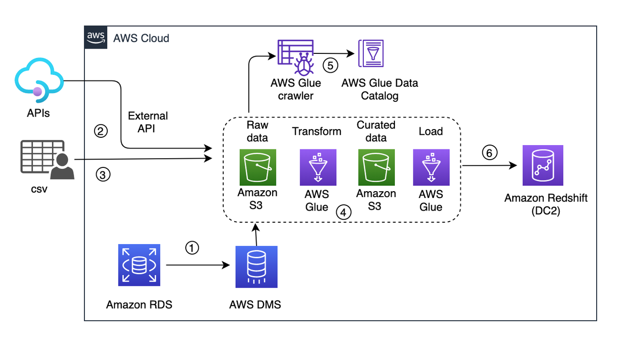
In this solution, data comes from three source systems and are written into a raw S3 bucket:

  • Change data capture (CDC) from an RDS instance via AWS DMS (1 in the preceding diagram)
  • Events captured via an external API (2)
  • CSV files from an external source copied to the raw bucket (3)

These sources don’t have a pattern or an interval of pushing new data.

Every few minutes, the ingested data is picked up by an S3 event trigger to run an AWS Glue workflow (4 in the preceding diagram). It provides an orchestration layer to manage and run jobs and crawlers. This workflow includes a crawler (5) that updates the metadata schema and partitions of the dataset to the AWS Glue Data Catalog. Then the crawler triggers an AWS Glue job that writes the curated data to the S3 curated bucket. From there, another AWS Glue job uploads data into Amazon Redshift (6).

In this scenario, if your workload is critical and you can’t afford a long downtime, then you need to plan your migration accordingly.

Dual write and transient data curation pipeline

As a first step of the migration, you need a parallel data process pipeline as the AWS Glue job, which writes the data into the curated S3 bucket. Create another S3 bucket and name it migrated-curated-bucket and modify the AWS Glue transform job. You can also replicate another transform job to write data to a new reserve S3 bucket in parallel.

In this scenario, live data ingestion occurs every 30 minutes. When an iteration of the extract, transform, and load (ETL) job is complete, this triggers a manual snapshot of the Amazon Redshift cluster. After the snapshot is captured, a new Amazon Redshift cluster is created using that snapshot. Cluster creation time can vary depending on the snapshot volume.

If snapshot creation takes more than 30 minutes, then the ETL job should be stopped, and resume after the snapshot creation is complete. For example, if the ETL job is triggered at 8:00 AM and finishes at 8:10 AM, then snapshot creation starts at 8:10 AM. If it finishes by 8:30 AM (the next ETL job will run at 8:30 AM as per the half-hour interval), then the ETL process continues according to the schedule. Otherwise, the job stops, and resumes after the snapshot completion.

Now we use the snapshot to launch a new RA3 redshift cluster. The process doesn’t pause the existing ETL pipeline, rather it starts writing curated data in parallel to the reserve S3 bucket. The following diagram illustrates this updated workflow.

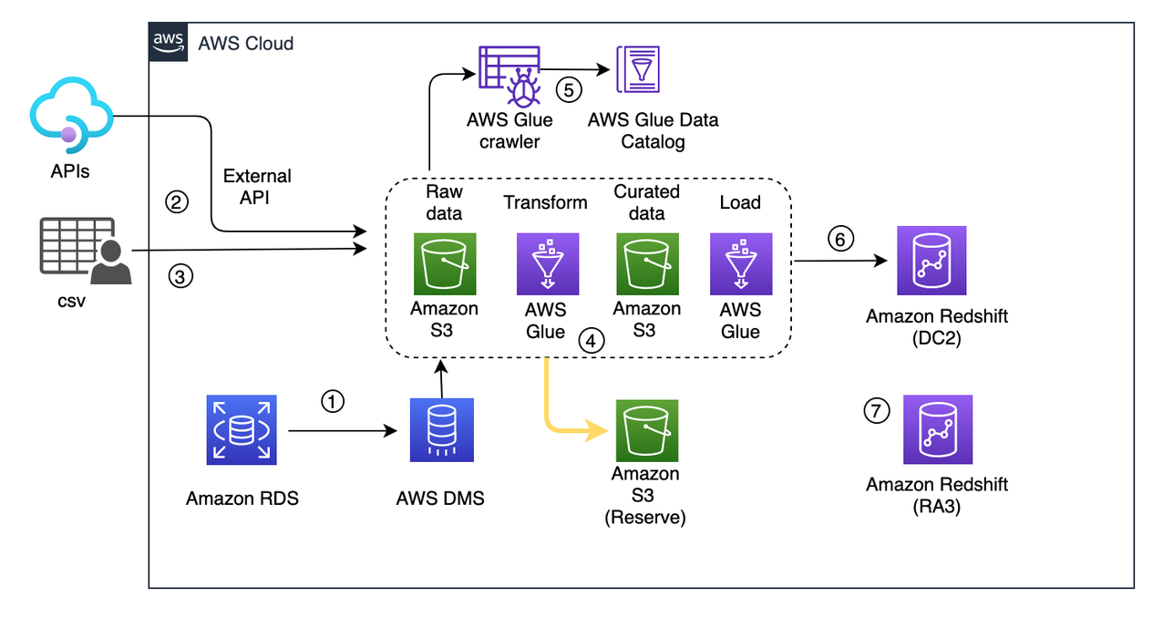
At this point, the existing cluster is still live and continues to process the live workload. Even if creation of the Amazon Redshift cluster takes time (owing to the huge volume of data), you should still be covered. The curated data in the S3 bucket acts as a staging reserve, and this data should be loaded into the RA3 cluster after its cluster is launched.

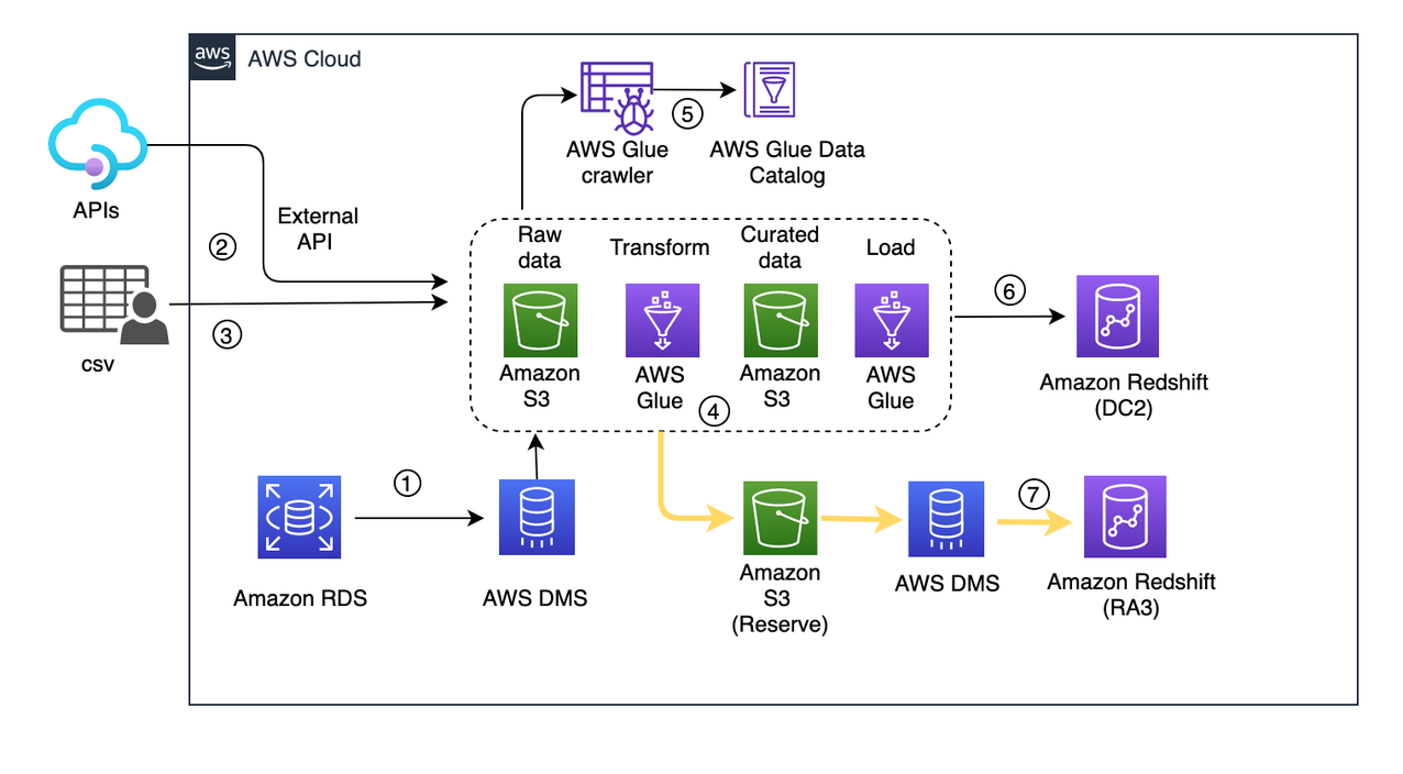
Backfill the new RA3 cluster with missing data

After the RA3 cluster has been launched, you need to playback the captured live data from the reserve S3 bucket to the newly created cluster. Playback is only for the duration of the snapshot capture to the current timestamp. With this process, you’re trying to bring the RA3 cluster in sync with the existing live DC2 cluster.

You need to configure an AWS DMS migration task with the reserve S3 bucket as the source endpoint and the newly created RA3 cluster as the target endpoint.

AWS DMS captures ongoing changes to the target data store. This process is called ongoing replication or change data capture (CDC). AWS DMS uses this process when replicating ongoing changes from a source data store. This process works by collecting changes to the database logs using the database engine’s native API. The following diagram illustrates this workflow.

Reconciliation and cutover

Data reconciliation is the process of verification of data between source and target. In this process, target data is compared with source data to ensure that the data is transferred completely without any alterations. To ensure reliability in the pipeline and the data processed, you should create an end-to-end reconciliation report. This report verifies the percentage of matching tables, columns, and data records. It also identifies missing records, missing values, incorrect values, badly formatted values, and duplicated records.

You can define the reconciliation process to check whether both clusters are running in sync. For that you can create simple Python scripts or shell scripts to query the source and target clusters, fetch the results, and compare.

Cutover is the final step of migration, and involves switching the existing cluster with the newly launched cluster. At this point, the clusters are running in parallel. Next, you validate that the downstream data consumption flows are up to date. Verify the reconciliation metrics from the DC2 and RA3 clusters such that table updates are in sync.

You can keep dual write while you switch from the migration data pipeline. If you discover any issues after cutting over, you can switch back to the old data pipeline, which is the source of truth until cutover. In this case, cutover involves updating the DC2 cluster endpoint to the new RA3 cluster endpoint in the application. Make sure to identify a relatively quiet window during  the day to update the endpoint. To keep the same endpoint for your applications and users, you can rename the new RA3 cluster with the same name as the original DC2 cluster. To rename the cluster, modify the cluster in the Amazon Redshift console or ModifyCluster API operation. For more information, see Renaming clusters or ModifyCluster API operation in the Amazon Redshift API Reference.

Up to this point, AWS DMS is continuing to update RA3. After you cut over to RA3, the DC2 cluster is no longer live and you can stop the AWS DMS replication job to RA3. Pause the last snapshot. Delete the reserve S3 bucket and AWS DMS resources used for RA3 load.

Conclusion

In this post, we presented an approach to migrate an existing Amazon Redshift cluster with minimal to no data loss, which also allows the cluster to serve both read and write operations during the resize window. Elastic resize is a quick way to resize your cluster to maintain the same number of slices in the target cluster. Slice mapping reduces the time required to resize a cluster. If you choose a resize configuration that isn’t available on elastic resize, you can choose classic resize or perform a snapshot, restore, and resize.

To learn more about what’s new with RA3 instances, refer to Amazon Redshift RA3 instances with managed storage. Amazon Redshift delivers better price performance and at the same time helps you keep your costs predictable. Amazon Redshift Serverless automatically provisions and scales the data warehouse capacity to deliver high performance for demanding and unpredictable workloads, and you pay only for the resources you use. This provides greater flexibility to choose either or both based on custom requirements. After you’ve made your choice, try the hands-on labs on Amazon Redshift.


About the Authors

Soujanya Konka is a Solutions Architect and Analytics specialist at AWS, focused on helping customers build their ideas on cloud. Expertise in design and implementation of business information systems and Data warehousing solutions. Before joining AWS, Soujanya has had stints with companies such as HSBC, Cognizant.

Dipayan Sarkar is a Specialist Solutions Architect for Analytics at AWS, where he helps customers to modernise their data platform using AWS Analytics services. He works with customer to design and build analytics solutions enabling business to make data-driven decisions.

Visualize MongoDB data from Amazon QuickSight using Amazon Athena Federated Query

Post Syndicated from Soujanya Konka original https://aws.amazon.com/blogs/big-data/visualize-mongodb-data-from-amazon-quicksight-using-amazon-athena-federated-query/

In this post, you will learn how to use Amazon Athena Federated Query to connect a MongoDB database to Amazon QuickSight in order to build dashboards and visualizations.

Amazon Athena is a serverless interactive query service, based on Presto, that provides full ANSI SQL support to query a variety of standard data formats, including CSV, JSON, ORC, Avro, and Parquet, that are stored on Amazon Simple Storage Service (Amazon S3). For data that isn’t stored on Amazon S3, you can use Athena Federated Query to query the data in place or build pipelines that extract data from multiple data sources and store it in Amazon S3. With Athena Federated Query, you can run SQL queries across data that is stored in relational, non-relational, object, and custom data sources.

MongoDB is a popular NoSQL database option for websites and API endpoints. You can choose to deploy MongoDB as a self-hosted or fully-managed database. Databases are a popular choice for UI applications for managing user profiles, product catalogs, profile views, clickstream events, events from a connected device, and so on. QuickSight is a serverless business analytics service with built-in machine learning (ML) capabilities that can automatically look for patterns and outliers, and has the flexibility to embed dashboards in applications for a data-driven experience. You can also use QuickSight Q to allow users to ask questions using natural language and find answers to business questions immediately.

Overview of Athena Federated Query

Athena Federated Query uses data source connectors that run on AWS Lambda to run federated queries to other data sources. Prebuilt data source connectors are available for native stores, like Amazon Timestream, Amazon CloudWatch Logs, Amazon DynamoDB, and external sources like Vertica and SAP Hana. You can also write a connector by using the Athena Query Federation SDK. You can customize Athena’s prebuilt connectors for your own use, or modify a copy of the source code to create your own AWS Serverless Application Repository package.

Solution overview

The following architecture diagram shows the components of the Athena Federated Query MongoDB connector. It contains the following components:

  • A virtual private cloud (VPC) configured with public and private subnets across three Availability Zones.
  • A MongoDB cluster with customizable Amazon Elastic Block Store (Amazon EBS) storage deployed in private subnets and NAT gateways in a public subnet for outbound internet connectivity for MongoDB instances.
  • Bastion hosts in an auto scaling group with Elastic IP addresses to allow inbound SSH access.
  • An AWS Identity and Access Management (IAM) MongoDBnode role with Amazon Elastic Compute Cloud (Amazon EC2) and Amazon S3 permissions.
  • Security groups to enable communication within the VPC.
  • Lambda functions deployed in a private subnet accessing S3 buckets. Athena invokes the Lambda function, which in turn fetches the data from MongoDB and maps the response back to Athena.
  • AWS Secrets Manager through a VPC endpoint.

Prerequisites

To implement the solution, you need the following:

  • An AWS account to access AWS services.
  • An IAM user with permission to CreateRole, ListRoles, GetPolicy, and AttachRolePolicy.
  • An IAM user with an access key and secret key to configure an integrated development environment (IDE).
  • A MongoDB database. You can deploy a hosted MongoDB on Amazon EC2 or MongoDB Atlas in a VPC.
  • If you don’t have a QuickSight subscription configured, sign up for one. You can access the QuickSight free trial as part of the AWS Free Tier option.
  • A new secret in Secrets Manager to store your MongoDB user name and password.
  • Data loaded into your MongoDB database. For this example, we used an airline dataset. Load the sample data either from the MongoDB command line or the MongoDB Atlas user interface, if using MongoDB Atlas.

Configure a Lambda connector

The first step in the deployment is to set up the connector environment. Athena uses data source connectors that run on Lambda to run federated queries. To connect with MongoDB, use the Amazon Athena DocumentDB Connector, which also works with any endpoint that is compatible with MongoDB.

To configure a Lambda connector, complete the following steps:

  1. On the Athena console, choose Data sources in the navigation pane.
  2. To view a published list of data sources for Athena, select Amazon DocumentDB.
  3. Choose Next.
  4. In the Data source details section, give your data source a unique name; for example, ds_mongo.
    This will be the connection name that appears under Data sources for Athena.
  5. Choose Create Lambda function.
    This launches the Create function page in Lambda. The connector is deployed by using AWS Serverless Application Repository.
  6. For SecretNameOrPrefix, enter mongo.
  7. For SpillBucket, enter spl-mongo-athena-test.
  8. For AthenaCatalogName, enter us-west-mongo-cat.
  9. For DocDBConnectionString (the MongoDB connection), enter the following:
    mongodb://${docdb_instance_1_creds}@replace_with_mongodb_private_ip:27017/?authSource=admin&readPreference=secondaryPreferred&retryWrites=false; 

  10. For SecurityGroupIds, choose the security group that you want to associate with the function. Make sure that the security group of the MongoDB instance allows traffic from the Lambda function.
  11. For SpillPrefix, enter athena-spill.
  12. For Subnetids, enter the subnet IDs of subnets with MongoDB instances.
    In this case, LambdaMemory and LambdaTimeout have been set to the maximum values, but these can vary depending on the query run and memory requirements. SpillBucket is an S3 bucket in your account to store data that exceeds the Lambda function response size limits.
  13. Keep the rest as defaults.
  14. Select the acknowledgement check box choose Deploy.
    The connection function is launched based on the given parameters.
  15. Create a VPC endpoint to allow the Lambda function to access Amazon S3 through an endpoint.
    This is for the spill bucket. The spill bucket is a staging area for copying the results of the queries that are performed on MongoDB via Athena federation. This is so that the Lambda function in the VPC can access Amazon S3.
  16. Go back to the Athena console.
  17. Under Connection details, for Lambda function, choose the newly created Lambda function.
  18. Choose Next.

  19. To verify the connection, on the Athena console, choose Data sources, then choose ds_mongo.
    Associated databases from the connection should be listed.

    You should now be able to query the datasets from the Athena query editor by using SQL.
  20. In the query editor, for Data Source, choose ds_mongo.

Athena federates the query using the connector, which invokes the Lambda function. Then the query is performed by the function on MongoDB, and the query results are translated back to Athena. The following is a sample query that was performed on the airlines dataset.

Create a dataset on QuickSight to read the data from MongoDB

Before you launch QuickSight for the first time in an AWS account, you must set up an account. For instructions, see Signing in to Amazon QuickSight.

After the initial setup, you can create a dataset with Athena as the source. The QuickSight service role needs permission to invoke the Lambda function that connects MongoDB. The aws-quicksight-service-role-v0 service role is automatically created with the QuickSight account.

To create a dataset in QuickSight, complete the following steps:

  1. On the IAM console, in the navigation pane, choose Roles.
  2. Search for the role aws-quicksight-service-role-v0 and add the permission Lambda _fullaccess.
    In an organization, there could be different data stores based on data load and consumption patterns. Examples include catalog or manual data that is associated with products in a MongoDB or key-value index store, transactions or sales data in a SQL database, and images or video clips that are associated with the product in an object store.
    In this case, an airlines table from MongoDB is joined with a flat file that contains information on the airports.
  3. Use the QuickSight cross-data store feature to join data from different sources on common fields.
  4. We then update the data types for our geographic fields like fields like city, country, latitude, and longitude so we can build maps later.
  5. You can also create calculated fields while preparing your dataset, which allows you to reuse them in other QuickSight analyses.

With a few clicks, you should be able to create a dashboard with the published dataset. For instance, you can plot your data on a map, show trends in a line chart, and add autonarratives from the list of Suggested Insights to create the analysis shown in the following screenshot.

Clean up

Make sure to clean up your resources to avoid resource spend and associated costs. You need to delete the EC2 instances with MongoDB. In the case of MongoDB Atlas, you can delete the databases and tables. Delete the Athena data source ds_mongo and unsubscribe your QuickSight account from the Manage QuickSight admin page.

Conclusion

With QuickSight and Athena Federated Query, organizations can access additional data sources beyond those already supported by QuickSight. If you have data in sources other than Amazon S3, you can use Athena Federated Query to analyze the data in place or build pipelines that extract and store data in Amazon S3. Athena now also supports cross-account federated queries to enable teams of analysts, data scientists, and data engineers to query data stored in other AWS accounts. Try connecting to proprietary data formats and sources, or build new user-defined functions, with the Athena Query Federation SDK.


About the Author

Soujanya Konka is a Solutions Architect and Analytics specialist at AWS, focused on helping customers build their ideas on cloud. Expertise in design and implementation of business information systems and Data warehousing solutions. Before joining AWS, Soujanya has had stints with companies such as HSBC, Cognizant.

Nilesh Parekh is a Partner Solution Architect with ISV India segment. Nilesh help assist partner to review and remediate their workload running on AWS based on the AWS Well-Architected and Foundational Technical Review best practices. He also helps assist partners on Application Modernizations and delivering POCs.

Migrate to an Amazon Redshift Lake House Architecture from Snowflake

Post Syndicated from Soujanya Konka original https://aws.amazon.com/blogs/big-data/migrate-to-an-amazon-redshift-lake-house-architecture-from-snowflake/

The need to derive meaningful and timely insights increases proportionally with the amount of data being collected. Data warehouses play a key role in storing, transforming, and making data easily accessible to enable a wide range of use cases, such as data mining, business intelligence (BI) and reporting, and diagnostics, as well as predictive, prescriptive, and cognitive analysis.

Several new features of Amazon Redshift address a wide range of data requirements and improve performance of extract, load, and transform (ELT) jobs and queries. For example, concurrency scaling, the new RA3 instance types, elastic resize, materialized views, and federated query, which allows you to query data stored in your Amazon Aurora or Amazon Relational Database Service (Amazon RDS) Postgres operational databases directly from Amazon Redshift, and the SUPER data type, which can store semi-structured data or documents as values. The new distributed and hardware accelerated cache with AQUA (Advanced Query Accelerator) for Amazon Redshift delivers up to10 times more performance than other cloud warehouses. The machine learning (ML) based self-tuning capability to set sort and distribution keys for tables significantly improves query performance that was previously handled manually. For the latest feature releases for AWS services, see What’s New with AWS?

To take advantage of these capabilities and future innovation, you need to migrate from your current data warehouse, like Snowflake, to Amazon Redshift, which involves two primary steps:

  • Migrate raw, transformed, and prepared data from Snowflake to Amazon Simple Storage Service (Amazon S3)
  • Reconfigure data pipelines to move data from sources to Amazon Redshift and Amazon S3, which provide a unified, natively integrated storage layer of our Lake House Architecture

In this post, we show you how to migrate data from Snowflake to Amazon Redshift. We cover the second step, reconfiguring pipelines, in a later post.

Solution overview

Our solution is designed in two stages, as illustrated in the following architecture diagram.

The first part of our Lake House Architecture is to ingest data into the data lake. We use AWS Glue Studio with AWS Glue custom connectors to connect to the source Snowflake database and extract the tables we want and store them in Amazon S3. To accelerate extracting business insights, we load the frequently accessed data into an Amazon Redshift cluster. The infrequently accessed data is cataloged in the AWS Glue Data Catalog as external tables that can be easily accessed from our cluster.

For this post, we consider three tables: Customer, Lineitem, and Orders, from the open-source TCPH_SF10 dataset. An AWS Glue ETL job, created by AWS Glue Studio, moves the Customers and Orders tables from Snowflake into the Amazon Redshift cluster, and the Lineitem table is copied to Amazon S3 as an external table. A view is created in Amazon Redshift to combine internal and external datasets.

Prerequisites

Before we begin, complete the steps required to set up and deploy the solution:

  1. Create an AWS Secrets Manager secret with the credentials to connect to Snowflake: username, password, and warehouse details. For instructions, see Tutorial: Creating and retrieving a secret.
  2. Download the latest Snowflake JDBC JAR file and upload it to an S3 bucket. You will find this bucket referenced as SnowflakeConnectionbucket in the cloudformation step.
  3. Identify the tables in your Snowflake database that you want to migrate.

Create a Snowflake connector using AWS Glue Studio

To complete a successful connection, you should be familiar with the Snowflake ecosystem and the associated parameters for Snowflake database tables. These can be passed as job parameters during run time. The following screenshot from a Snowflake test account shows the parameter values used in the sample job.

The following screenshot shows the account credentials and database from Secrets Manager.

To create your AWS Glue custom connector for Snowflake, complete the following steps:

  1. On the AWS Glue Studio console, under Connectors, choose Create custom connector.
  2. For Connector S3 URL, browse to the S3 location where you uploaded the Snowflake JDBC connector JAR file.
  3. For Name, enter a logical name.
  4. For Connector type, choose JDBC.
  5. For Class name, enter net.snowflake.client.jdbc.SnowflakeDriver.
  6. Enter the JDBC URL base in the following format: jdbc:snowflake://<snowflakeaccountinfo>/?user=${Username}&password=${Password}&warehouse=${warehouse}.
  7. For URL parameter delimiter, enter &.
  8. Optionally, enter a description to identify your connector.
  9. Choose Create connector.

Set up a Snowflake JDBC connection

To create a JDBC connection to Snowflake, complete the following steps:

  1. On the AWS Glue Studio console, choose Connectors.
  2. Choose the connector you created.
  3. Choose Create connection.

  4. For Name and Description, enter a logical name and description for your reference.
  5. For Connection credential type, choose default.
  6. For AWS Secret, choose the secret created as a part of the prerequisites.
  7. Optionally, you can specify the credentials in plaintext format.
  8. Under Additional options, add the following key-value pairs:
    1. Key db with the Snowflake database name
    2. Key schema with the Snowflake database schema
    3. Key warehouse with the Snowflake warehouse name
  9. Choose Create connection.

Configure other resources and permissions using AWS CloudFormation

In this step, we create additional resources with AWS CloudFormation, which includes an Amazon Redshift cluster, AWS Identity and Access Management (IAM) roles with policies, S3 bucket, and AWS Glue jobs to copy tables from Snowflake to Amazon S3 and from Amazon S3 to Amazon Redshift.

  1. Sign in to the AWS Management Console as an IAM power user, preferably an admin user.
  2. Choose your Region as us-east-1.
  3. Choose Launch Stack:
  4. Choose Next.
  5. For Stack name, enter a name for the stack, for example, snowflake-to-aws-blog.
  6. For Secretname, enter the secret name created in the prerequisites.
  7. For SnowflakeConnectionName, enter the Snowflake JDBC connection you created.
  8. For Snowflake Connection bucket, enter name of the S3 bucket where the snowflake connector is uploaded
  9. For SnowflakeTableNames, enter the list of tables to migrate from Snowflake. For example, Lineitem,customers,order.
  10. For RedshiftTableNames, enter the list of the tables to load into your warehouse (Amazon Redshift). For example, customers,order.
  11. You can specify your choice of Amazon Redshift node type, number of nodes, and Amazon Redshift username and password, or use the default values.
  12. For the MasterUserPassword, enter a password for your master user keeping in mind the following constraints : It must be 8 to 64 characters in length. It must contain at least one uppercase letter, one lowercase letter, and one number.
  13. Choose Create stack.

Run AWS Glue jobs for the data load

The stack takes about 7 minutes to complete. After the stack is deployed successfully, perform the following actions:

  1. On the AWS Glue Studio console, under Databases, choose Connections.
  2. Select the connection redshiftconnection from the list and choose Test Connection.
  3. Choose the IAM role ExecuteGlueSnowflakeJobRole from the drop-down meu and choose Test connection.

If you receive an error, verify or edit the username and password and try again.

  1. After the connection is tested successfully, on the AWS Glue Studio console, select the job Snowflake-s3-load-job.
  2. On the Action menu, choose Run job.

When the job is complete, all the tables mentioned in the SnowflakeTableNames parameter are loaded into your S3 bucket. The time it takes to complete this job varies depending on the number and size of the tables.

Now we load the identified tables in Amazon Redshift.

  1. Run the job s3-redshift-load-job.
  2. After the job is complete, navigate to the Amazon Redshift console.
  3. Use the query editor to connect to your cluster to verify that the tables specified in RedshiftTableNames are loaded successfully.

You can now view and query datasets from Amazon Redshift. The Lineitem dataset is on Amazon S3 and queried by Amazon Redshift Spectrum. The following screenshot shows how to create an Amazon Redshift external schema that allows you to query Amazon S3 data from Amazon Redshift.

Tables loaded to Amazon Redshift associated storage appear as in the following screenshot.

The AWS Glue job, using the standard worker type to move Snowflake data into Amazon S3, completed in approximately 21 minutes, loading overall 2.089 GB (about 76.5 million records). The following screenshot from the Snowflake console shows the tables and their sizes, which we copied to Amazon S3.

You have the ability to customize the AWS Glue worker type, worker nodes, and max concurrency to adjust distribution and workload.

AWS Glue allows parallel data reads from the data store by partitioning the data on a column. You must specify the partition column, the lower partition bound, the upper partition bound, and the number of partitions. This feature enables you use data parallelism and multiple Spark executors allocated the Spark application.

This completes our migration from Snowflake to Amazon Redshift that enables a Lake House Architecture and the ability to analyze data in more ways. We would like to take a step further and talk about features of Amazon Redshift that can help extend this architecture for data democratization and modernize your data warehouse.

Modernize your data warehouse

Amazon Redshift powers the Lake House Architecture, which enables queries from your data lake, data warehouse, and other stores. Amazon Redshift can access the data lake using Redshift Spectrum. Amazon Redshift automatically engages nodes from a separate fleet of Redshift Spectrum nodes. These nodes run queries directly against Amazon S3, run scans and aggregations, and return the data to the compute nodes for further processing.

AWS Lake Formation provides a governance solution for data stored in an Amazon S3-based data lake and offers a central permission model with fine-grained access controls at the column and row level. Lake Formation uses the AWS Glue Data Catalog as a central metadata repository and makes it simple to ingest and catalog data using blueprints and crawlers.

The following screenshot shows the tables from Snowflake represented in the AWS Glue Data Catalog and managed by Lake Formation.

With the Amazon Redshift data lake export feature, you can also save data back in Amazon S3 in open formats like Apache Parquet, to use with other analytics services like Amazon Athena and Amazon EMR.

Distributed storage

Amazon Redshift RA3 gives the flexibility to scale compute and storage independently. Amazon Redshift data is stored on Amazon Redshift managed storage backed by Amazon S3. Distribution of datasets between cluster storage and Amazon S3 allows you to benefit from bringing the appropriate compute to the data depending on your use case. You can query data from Amazon S3 without accessing Amazon Redshift.

Let’s look at an example with the star schema. We can save a fact table that we expect to grow rapidly in Amazon S3 with the schema saved in the Data Catalog, and dimension tables in cluster storage. You can use views with union data from both Amazon S3 and the attached Amazon Redshift managed storage.

Another model for data distribution can be based on the state of hot or cold data, with hot data in Amazon Redshift managed storage and cold data in Amazon S3. In this example, we have the datasets lineitem, customer, and orders. The customer and orders portfolio are infrequently updated datasets in comparison to lineitem. We can create an external table to read lineitem data from Amazon S3 and the schema from the Data Catalog database, and load customer and orders to Amazon Redshift tables. The following screenshot shows a join query between the datasets.

It would be interesting to know the overall run statistics for this query, which can be queried from system tables. The following code gets the stats from the preceding query using svl_s3query_summary:

select elapsed, s3_scanned_rows, s3_scanned_bytes,
s3query_returned_rows, s3query_returned_bytes, files, avg_request_parallelism
from svl_s3query_summary
where query = 1918
order by query,segment;

The following screenshot shows query output.

For more information about this query, see Using the SVL_QUERY_SUMMARY view.

Automated table optimization

Distribution and sort keys are table properties that define how data is physically stored. These are managed by Amazon Redshift. Automatic table optimization continuously observes how queries interact with tables and uses ML to select the best sort and distribution keys to optimize performance for the cluster’s workload. To enhance performance, Amazon Redshift chooses the key and tables are altered automatically.

In the preceding scenario, the lineitem table had distkey (L_ORDERKEY), the customer table had distribution ALL, and orders had distkey (O_ORDERKEY).

Storage optimization

Choosing a data format depends on the data size (JSON, CSV, or Parquet). Redshift Spectrum currently supports Avro, CSV, Grok, Amazon Ion, JSON, ORC, Parquet, RCFile, RegexSerDe, Sequence, Text, and TSV data formats. When you choose your format, consider the overall data scanned and I/O efficiency, such as with a small dataset in CSV or JSON format versus the same dataset in columnar Parquet format. In this case, for smaller scans, Parquet consumes more compute capacity compared to CSV, and may eventually take around the same time as CSV. In most cases, Parquet is the optimal choice, but you need to consider other inputs like volume, cost, and latency.

SUPER data type

The SUPER data type offers native support for semi-structured data. It supports nested data formats such as JSON and Ion files. This allows you to ingest, store, and query nested data natively in Amazon Redshift. You can store JSON formatted data in SUPER columns.

You can query the SUPER data type through an easy-to-use SQL extension that is powered by the PartiQL. PartiQL is a SQL language that makes it easy to efficiently query data regardless of the format, whether the data is structured or semi-structured.

Pause and resume

Pause and resume lets you easily start and stop a cluster to save costs for intermittent workloads. This way, you can cost-effectively manage a cluster with infrequently accessed data.

You can apply pause and resume via the console, API, and user-defined schedules.

AQUA

AQUA for Amazon Redshift is a large high-speed cache architecture on top of Amazon S3 that can scale out to process data in parallel across many nodes. It flips the current paradigm of bringing the data to the compute—AQUA brings the compute to the storage layer so the data doesn’t have to move back and forth between the two, which enables Amazon Redshift to run queries much faster.

Data sharing

The data sharing feature seamlessly allows multiple Amazon Redshift clusters to query data located in RA3 clusters and their managed storage. This is ideal for workloads that are isolated from each other but data needs to be shared for cross-group collaboration without actually copying data.

Concurrency scaling

Amazon Redshift automatically adds transient clusters in seconds to serve sudden spikes in concurrent requests with consistently fast performance. For every 1 day of usage, 1 hour of concurrency scaling is available at no charge.

Conclusion

In this post, we discussed an approach to migrate a Snowflake data warehouse to a Lake House Architecture with a central data lake accessible through Amazon Redshift.

We covered how to use AWS Glue to move data from sources like Snowflake into your data lake, catalog it, and make it ready to analyze in a few simple steps. We also saw how to use Lake Formation to enable governance and fine-grained security in the data lake. Lastly, we discussed several new features of Amazon Redshift that make it easy to use, perform better, and scale to meet business demands.


About the Authors

Soujanya Konka is a Solutions Architect and Analytics specialist at AWS, focused on helping customers build their ideas on cloud. Expertise in design and implementation of business information systems and Data warehousing solutions. Before joining AWS, Soujanya has had stints with companies such as HSBC, Cognizant.

Shraddha Patel is a Solutions Architect and Big data and Analytics Specialist at AWS. She works with customers and partners to build scalable, highly available and secure solutions in the AWS cloud.