When we built AWS Glue interactive sessions, our goal was to make AWS Glue as interactive as running local Python from a notebook. We mostly succeeded. With a straightforward Python package and a Jupyter notebook, you could execute remotely against the AWS Glue ephemeral Spark backend. The Livy-based approach was ahead of its time, but it had limitations from its REST-based protocol. Running local PySpark unlocked powerful integrated development environment (IDE) features such as debugging and linting, so your environment could understand the code and help you develop Spark applications more quickly. Customers would often split their development work. They used local Spark (or Docker containers) to develop in an IDE on a small amount of data, then switched to AWS Glue interactive sessions to validate scaling and tuning against the full dataset.
With modern PySpark releases came a new protocol: Apache Spark Connect. Spark Connect bridges the gap between these two worlds: you develop in local Python, but execute on AWS Glue against actual data. Today, AWS Glue interactive sessions support Spark Connect natively. You can connect from any environment that supports the PySpark remote() API, including VS Code, PyCharm, Amazon SageMaker Unified Studio notebooks, and standalone Python applications. You don’t need to install specialized kernels or manage cluster infrastructure.
What Spark Connect changes
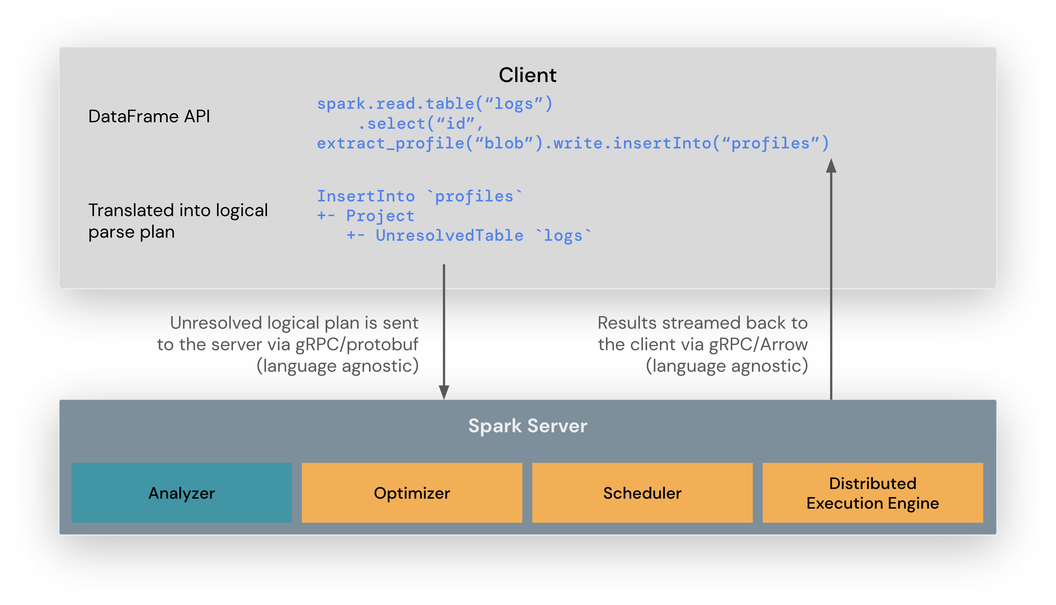
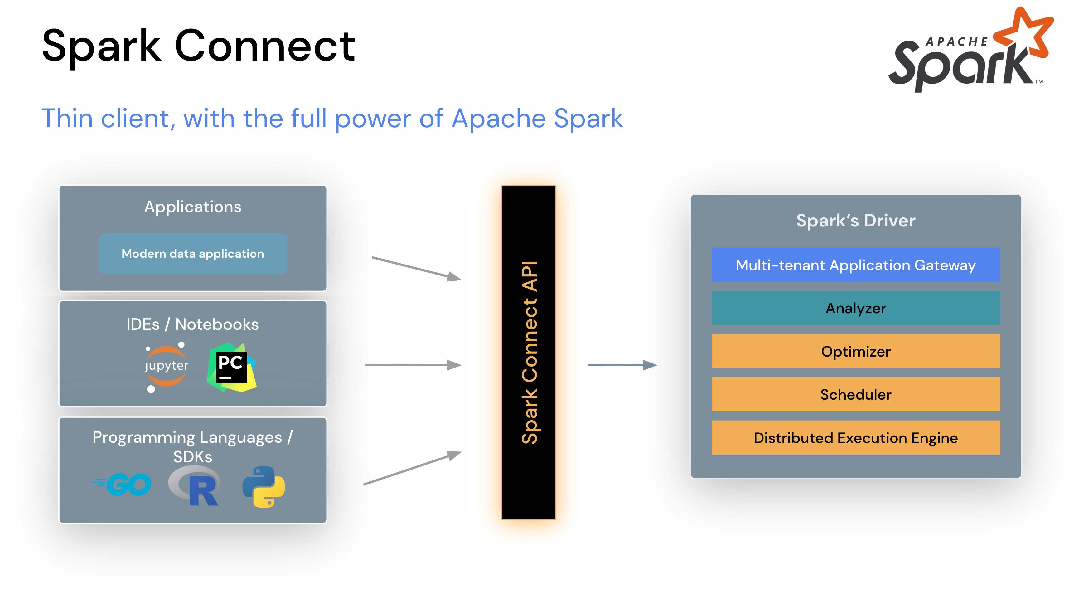
Spark Connect, introduced in Spark 3.4, decouples the Spark client from the server through a lightweight gRPC protocol. Instead of running your driver program on the cluster, your IDE communicates with a remote Spark server through a thin client layer. This architecture unlocks the key workflow improvement: you develop locally and execute remotely.
Spark Connect architecture — thin client with the full power of Apache Spark
With Spark Connect support in AWS Glue interactive sessions, you get:
IDE freedom – Use VS Code, PyCharm, JupyterLab, or any Python environment. No kernel installation required.
Programmatic access – Build Spark into your Python applications and automation scripts with a standard SparkSession.builder.remote() call.
Serverless execution – AWS Glue provisions and manages the Spark cluster. You pay only for the data processing units (DPUs) consumed while your session is active.
Spark Connect monitoring – The Spark Live UI now includes a dedicated Connect tab showing active Spark Connect sessions and operations alongside the existing Jobs, Stages, and Executors views.
Getting started with SageMaker Unified Studio
Amazon SageMaker Unified Studio provides the most direct path to Spark Connect on AWS Glue. The notebook environment handles session creation, endpoint retrieval, and token refresh automatically, so no connection boilerplate is required.
Prerequisite: You need an Amazon SageMaker Unified Studio project to use this workflow. If you don’t have one, create a project in your SageMaker Unified Studio domain first.
To connect to an AWS Glue Spark Connect session:
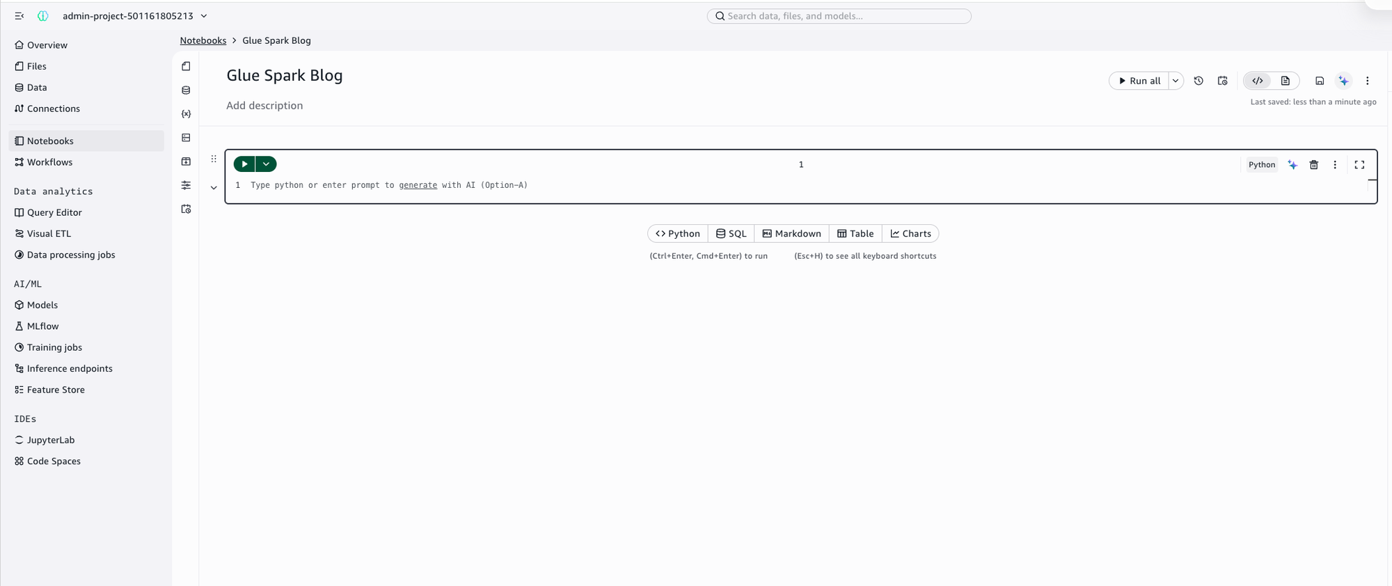
Sign in to SageMaker Unified Studio, choose your project, and create or open a Notebook.
A notebook open in SageMaker Unified Studio
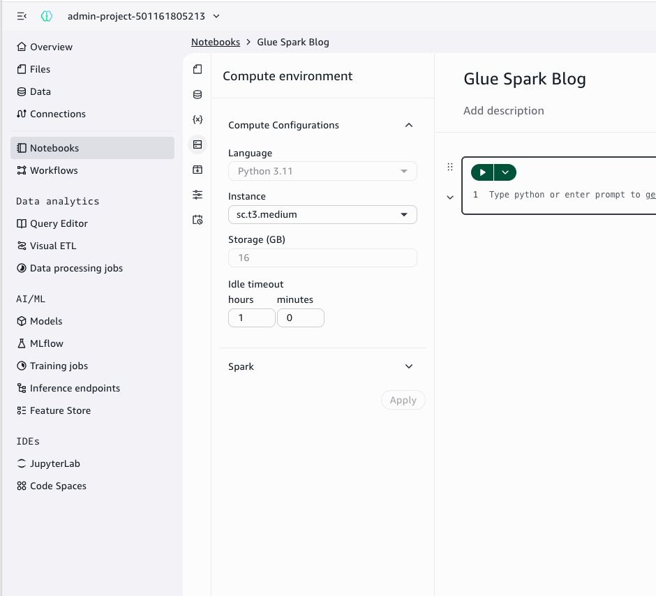
Choose the compute icon in the left toolbar to open the Compute environment panel. Expand the Spark section.
The Compute environment panel with the Spark dropdown list
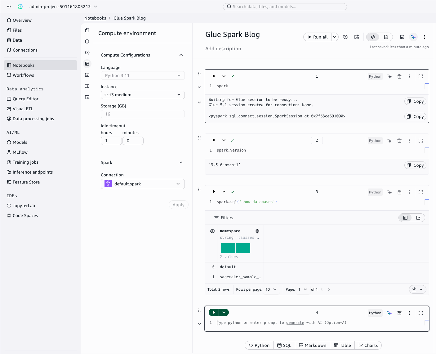
Select a Glue Spark connection. Depending on your SageMaker domain configuration, you will see either default.spark or named connections such as project.spark.compatibility. Select the appropriate Glue (Spark) connection and choose Apply.
Connected to Glue Spark Connect — running spark.version returns ‘3.5.6-amzn-1’
After you make your selection, you’re connected. The spark session object is available natively. No imports or configuration are needed. Start running PySpark immediately:
spark.sql("SHOW DATABASES").show()
The session manages itself in the background, including automatic token refresh.
Using the sagemaker_studio SDK
The sagemaker-studio Python package extends the Spark Connect experience beyond SageMaker Unified Studio notebooks into local IDEs, continuous integration and continuous delivery (CI/CD) pipelines, and any Python environment. The sparkutils module handles session initialization and connection configuration in a single call. You get the same streamlined experience as in the notebook, anywhere you run Python:
from sagemaker_studio import sparkutils

# Initialize a Glue Spark Connect session using your project connection
spark = sparkutils.init(connection_name="default.spark")

# Run queries immediately
spark.sql("SHOW DATABASES").show()
You can also use sparkutils.get_spark_options() to retrieve pre-configured Java Database Connectivity (JDBC) options for reading and writing to data sources through your project connections. Supported sources include Amazon Redshift, Amazon Aurora, and Amazon DocumentDB (with MongoDB compatibility):
# Get connection options for a Redshift connection in your project
options = sparkutils.get_spark_options("my_redshift_connection")

# Read from Redshift via Spark Connect
df = spark.read.format("jdbc").options(**options).option("dbtable", "analytics.orders").load()
df.show()
Within SageMaker Unified Studio, the sagemaker-studio SDK is native to the environment. The spark session and sparkutils are available without installation. For local IDE use, install it with pip install sagemaker-studio and configure credentials through an AWS named profile or boto3 session.
How it works
Spark Connect sessions in AWS Glue use a three-step workflow:
Create a session – Call the CreateSession API with SessionType set to SPARK_CONNECT. The session provisions in approximately 30 seconds.
Retrieve the endpoint – Call GetSessionEndpoint to receive a sc:// gRPC endpoint URL and a time-limited authentication token.
Connect with PySpark – Pass the endpoint and token to SparkSession.builder.remote() and start running Spark operations.
Spark Connect protocol flow — DataFrame API translated to logical plan, sent via gRPC/protobuf, results streamed back via gRPC/Arrow
Connecting with the low-level API
Some environments don’t have the sagemaker-studio SDK, such as custom containers, AWS Lambda functions, or non-Python toolchains. In these environments, or if you’re not using SageMaker Unified Studio, you can use the AWS SDK (Boto3) to manage sessions directly. The following example demonstrates the full workflow:
import time, boto3, urllib.parse
from pyspark.sql import SparkSession

glue = boto3.client("glue", region_name="us-east-1")

# 1. Create a Spark Connect session
session_id = "my-spark-connect-session"
glue.create_session(
    Id=session_id,
    Role="arn:aws:iam::123456789012:role/GlueServiceRole",
    Command={"Name": "glueetl"},
    GlueVersion="5.1",
    SessionType="SPARK_CONNECT",
    DefaultArguments={"--enable-spark-live-ui": "true"},
)

# 2. Wait for the session to reach READY
while True:
    status = glue.get_session(Id=session_id)["Session"]["Status"]
    if status == "READY":
        break
    time.sleep(5)

# 3. Get the Spark Connect endpoint
sc = glue.get_session_endpoint(SessionId=session_id)["SparkConnect"]
endpoint_url = sc["Url"]
auth_token = sc["AuthToken"]

# 4. Connect with PySpark
encoded_token = urllib.parse.quote(auth_token, safe="")
connection_string = f"{endpoint_url}:443/;use_ssl=true;x-aws-proxy-auth={encoded_token}"
spark = SparkSession.builder.remote(connection_string).getOrCreate()
spark.sql("SELECT 1 + 1 AS result").show()
Monitoring with Spark Live UI
When you enable the Spark Live UI at session creation, you gain access to a real-time dashboard showing:
Jobs and Stages – Track active, completed, and failed jobs with stage-level metrics.
Executors – Monitor memory usage, shuffle data, and executor health.
SQL – Inspect query plans and execution details.
Connect tab – View active Spark Connect sessions and operations (specific to Spark Connect).
Access the dashboard through the GetDashboardUrl API or directly from the AWS Glue console.
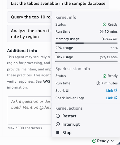
In SageMaker Unified Studio, no API call is needed. Choose Ready in the notebook status bar to open the kernel info popover. From there, open the Spark UI link for the live dashboard or Spark Driver Logs for real-time log output.
Image showing “Ready” in the status bar to access Spark UI and Driver Logs directly from the notebook
Token refresh
Authentication tokens expire after 30 minutes. In SageMaker Unified Studio, this is handled automatically. For programmatic use, you can use a background thread to keep the connection alive. The following helper reconnects transparently before the token expires:
import threading, time, boto3, urllib.parse
from pyspark.sql import SparkSession

class GlueSparkConnect:
    """Maintains a SparkSession with automatic token refresh."""

    def __init__(self, session_id, region="us-east-1", refresh_margin=300):
        self.session_id = session_id
        self.glue = boto3.client("glue", region_name=region)
        self.refresh_margin = refresh_margin  # seconds before expiry to refresh
        self._lock = threading.Lock()
        self.spark = self._connect()
        self._start_refresh_loop()

    def _connect(self):
        sc = self.glue.get_session_endpoint(SessionId=self.session_id)["SparkConnect"]
        encoded_token = urllib.parse.quote(sc["AuthToken"], safe="")
        remote_url = f"{sc['Url']}:443/;use_ssl=true;x-aws-proxy-auth={encoded_token}"
        self._token_expiry = sc["AuthTokenExpirationTime"].timestamp()
        return SparkSession.builder.remote(remote_url).getOrCreate()

    def _start_refresh_loop(self):
        def _loop():
            while True:
                sleep_for = max(self._token_expiry - time.time() - self.refresh_margin, 30)
                time.sleep(sleep_for)
                with self._lock:
                    self.spark = self._connect()
        t = threading.Thread(target=_loop, daemon=True)
        t.start()

# Usage
session = GlueSparkConnect("my-spark-connect-session")
session.spark.sql("SELECT 1 + 1 AS result").show()
The background thread sleeps until 5 minutes before token expiry, then transparently reconnects. Because the daemon thread exits when your script ends, there is no cleanup required.
Getting started
To start using Spark Connect with AWS Glue interactive sessions:
Grant your AWS Identity and Access Management (IAM) identity permissions for glue:CreateSession, glue:GetSession, and glue:GetSessionEndpoint.
Create a session with --session-type SPARK_CONNECT and connect from your preferred environment.
VPC note: If you connect to AWS Glue interactive sessions through a virtual private cloud (VPC) endpoint, add the new Spark Connect endpoint (com.amazonaws.{region}.glue.sessions) to your VPC configuration. Existing AWS Glue VPC endpoints don’t cover Spark Connect traffic.
For detailed instructions, see Connecting to a Spark Connect session in the AWS Glue Developer Guide.
AI coding assistants are transforming software development, but data engineering presents unique challenges: governed data access, shared compute environments, and compliance controls that are designed to remain in place. How do you bring the power of agentic AI development into a governed data environment? With the AWS Toolkit for Visual Studio Code, you can connect Kiro, VS Code, or Cursor directly to Amazon SageMaker Unified Studio.
When you connect your editor to a SageMaker Unified Studio Space (a cloud-based compute environment inside your project), you get AI-assisted development with your preferred tools while your data governance, project permissions, and compute are managed by SageMaker Unified Studio. Additionally, SageMaker Unified Studio automatically generates steering files (like AGENTS.md) that provide your AI assistant with context about your project environment, so it understands your data and project configuration from the first prompt.
This post demonstrates the integration using Kiro. The same Remote Access connection works with VS Code and Cursor. The post starts by showing what you can do with this integration: using natural language to explore and analyze data in a governed environment. We then walk through the setup so you can try it yourself.
What’s new
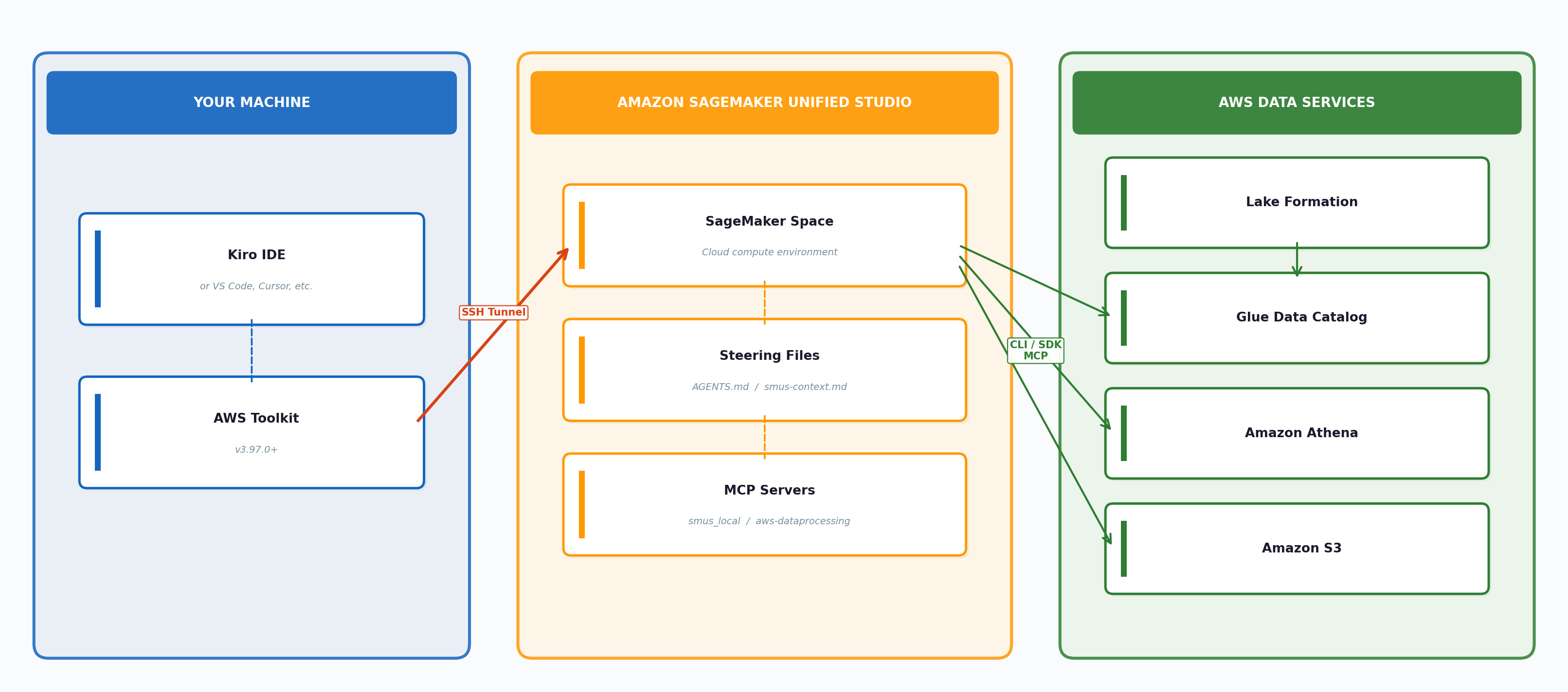
With the AWS Toolkit, you can connect Kiro, VS Code, and Cursor to your SageMaker Space over a secure SSH tunnel. No additional extensions or SSH key management required. After the connection is established, your IDE has full access to your Space’s file system, compute, and data services.
Two capabilities make this especially powerful for data work:
Automatic AI steering – When connecting Kiro to SageMaker Unified Studio, Kiro generates AGENTS.md and smus-context.md files that provide your AI assistant with context about your environment, including project configuration, environment details, and utilities for discovering your data catalog and project structure. Kiro detects these files automatically; other editors can use them as context for their own AI features.
MCP server support – have Kiro discover and configure itself for the Model Context Protocol servers on your remote SageMaker space ( like smus_local and aws-dataprocessing) to give your agent direct access to your AWS Glue Data Catalog, Amazon Athena queries, and SageMaker Unified Studio project metadata.
The following diagram shows how the components connect:
Architecture diagram: How the components connect
See it in action: AI-assisted development with governed data
Before walking through the setup, we explain what you can do with this integration. This walkthrough uses Kiro as the editor. With Kiro connected to a SageMaker Unified Studio Space, MCP servers configured, and steering documents in place, we can use natural language to explore data and build analytics. The AI assistant has all the context it needs to do this well.
Note: Agentic AI output is nondeterministic. The exact code, tool choices, and responses Kiro produces will vary between sessions, even with the same prompt. The following walkthrough shows one representative session. Your experience will differ in the specifics, but the patterns and capabilities demonstrated here are consistent.
Step 1: Explore the data
Start with a simple prompt:
show my databases and the tables I have access to
Even with native MCP tools available, Kiro often prefers the AWS Command Line Interface (AWS CLI) and bash to retrieve information. This is expected and typically does not affect the outcome. If you prefer MCP tools for every operation, you can add that preference to a steering document.
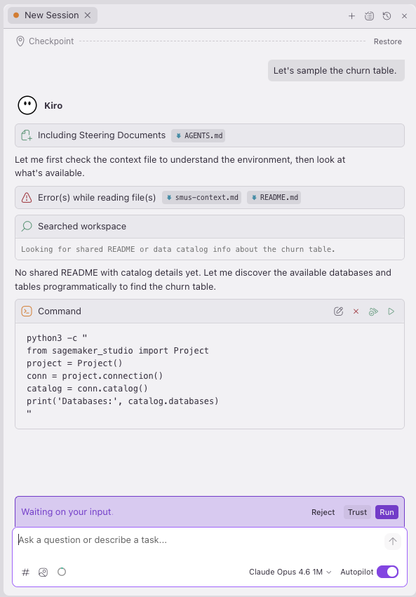
Kiro used the sagemaker_studio SDK to discover the catalog:
python3 -c "
from sagemaker_studio import Project
project = Project()
conn = project.connection()
catalog = conn.catalog()
print('Databases:')
for db in catalog.databases:
    print(f'  - {db.name}')
"
Databases:
  - default
  - sagemaker_sample_db
Then it drilled into the table schema:
python3 -c "
from sagemaker_studio import Project
project = Project()
conn = project.connection()
catalog = conn.catalog()
db = catalog.database('sagemaker_sample_db')
print('Tables in sagemaker_sample_db:')
for t in db.tables:
    print(f'  - {t.name}')
    print(f'    Columns: {[(c.name, c.type) for c in t.columns]}')
"
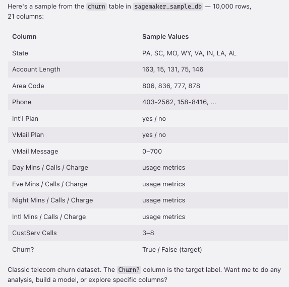
Kiro discovered the sagemaker_sample_db.churn dataset, a sample dataset that ships with SageMaker Unified Studio containing 10,000 rows and 21 columns of customer churn data (state, account length, call minutes, service calls, churn flag, and more). Notice that we did not write any of this code. We asked a question in natural language, and Kiro chose the right SDK calls, explored the catalog, and surfaced the results.
Another, more natural way to get the same answer is to ask directly. Prompting “Let us sample the churn table.” yields the same catalog paths and schema output, along with additional metrics like row count and a data sample, all from a single conversational prompt:
Figure 1 — The sagemaker_sample_db.churn dataset in the catalog
Figure 2 — Churn dataset schema with 21 columns
from sagemaker_studio import sqlutils
result = sqlutils.sql(
    'SELECT COUNT(*) AS total_rows FROM sagemaker_sample_db.churn',
    connection_name='default.sql'
)
print('=== Total Row Count ===')
print(result)
=== Total Row Count ===
   total_rows
0       10000
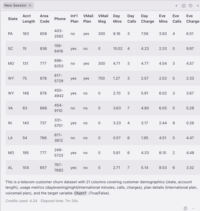
With the schema and row count in hand, Kiro sampled the data to round out its understanding of the dataset:
Figure 3 — Comprehensive data sample after Kiro catalog exploration
Step 2: Run analytics with full context
With the data explored, ask Kiro to run a data quality evaluation:
Can we run basic statistical evaluations for data quality?
Because Kiro had already explored the catalog and sampled the data, it made smart choices about how to run the analysis. Instead of using PySpark for this 10,000-row table, Kiro used Athena using sqlutils to run the evaluation directly. It produced a thorough data quality report:
10,000 rows, 21 columns, zero nulls across all columns. Clean on that front.
5,000 duplicate rows (50 percent). Significant, worth investigating before modeling.
Outliers minimal. Most columns have less than 1 percent outlier rate by IQR.
Clear signal in key features. Churners and non-churners show differences in day_mins (7.52 vs. 3.52), eve_mins (5.95 vs. 4.11), and vmail_message (175 vs. 278).
State distribution roughly uniform (~2% each), intl_plan and vmail_plan near 50/50.
The key insight here is what Kiro did not do. It did not default to PySpark because the environment supports Spark. Having explored the data first, understanding the table size, column types, and that churn is a proper Boolean (not a string), Kiro independently chose the right engine for the workload and produced correct analytics on the first pass.
Best practice: Explore first, code second
Start every AI-assisted development session with data exploration. Ask your AI assistant to discover your catalog, sample your tables, and understand the schema before asking it to build anything. This single step helps reduce a common source of errors in AI-assisted data work: the LLM making assumptions about data it has not seen.
Exploring your data gives the large language model (LLM) the context it needs to properly help with your project. It saves hallucinations and rework, results in faster development time, and reduces token costs.
Ready to try it yourself? The following sections walk through the full setup: prerequisites, connecting your editor to your SageMaker Space, configuring MCP servers, and working with notebooks.
Prerequisites
Before you begin, make sure you have the following:
A SageMaker Unified Studio domain and project with at least one project that has a compute environment provisioned (Tooling or ToolingLight). These should come standard with every SageMaker project except those provisioned with the SQL & Gen AI blueprints. If you need to set up SageMaker Unified Studio, see Getting started with Amazon SageMaker Unified Studio.
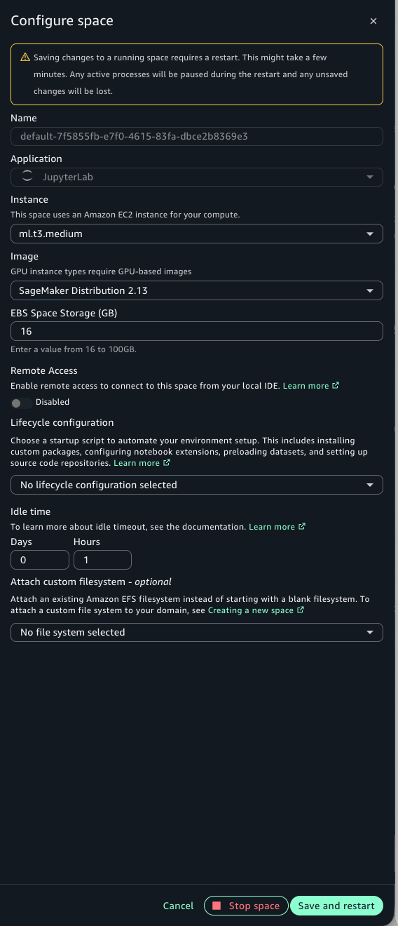
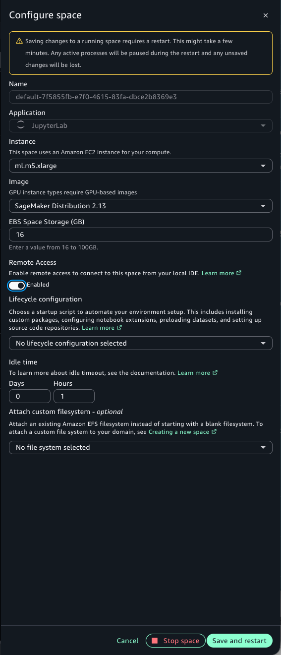
A Space with Remote Access enabled. Either a JupyterLab or Code Editor Space works. The instance must have at least 8 GiB of memory (for example, ml.t3.large or larger). The default ml.t3.medium (4 GiB) can’t enable Remote Access. You must upgrade the instance type first, then toggle Remote Access to Enabled in the Configure Space dialog.
A VS Code-compatible editor. Kiro, VS Code, Cursor, or another VS Code-based IDE installed on your local machine. This walkthrough uses Kiro, but the Remote Access connection has been tested with VS Code and Cursor as well.
AWS Toolkit v4.1.0 or later. Kiro ships with the AWS Toolkit pre-installed. For VS Code and Cursor, install the AWS Toolkit extension and verify your version is 4.1.0 or later (Cmd+Shift+X and search for “AWS Toolkit”).
AWS credentials. You must be authenticated in the SageMaker Unified Studio panel of the AWS Toolkit with the same identity (AWS IAM Identity Center or AWS Identity and Access Management (IAM)) that you use to access SageMaker Unified Studio in the browser.
Network connectivity. Your Space must have internet access (PublicInternetOnly mode, or virtual private cloud (VPC) with a NAT gateway or HTTP proxy that allows VS Code and Open VSX endpoints).
The following screenshots show the SageMaker Unified Studio portal and the Configure Space dialog. Navigate to your project, select your Space, and verify the configuration. Remote Access is disabled when the instance has less than 8 GiB of memory. Select an instance with at least 8 GiB, such as ml.t3.large, then enable Remote Access. This is a one-time configuration per Space.
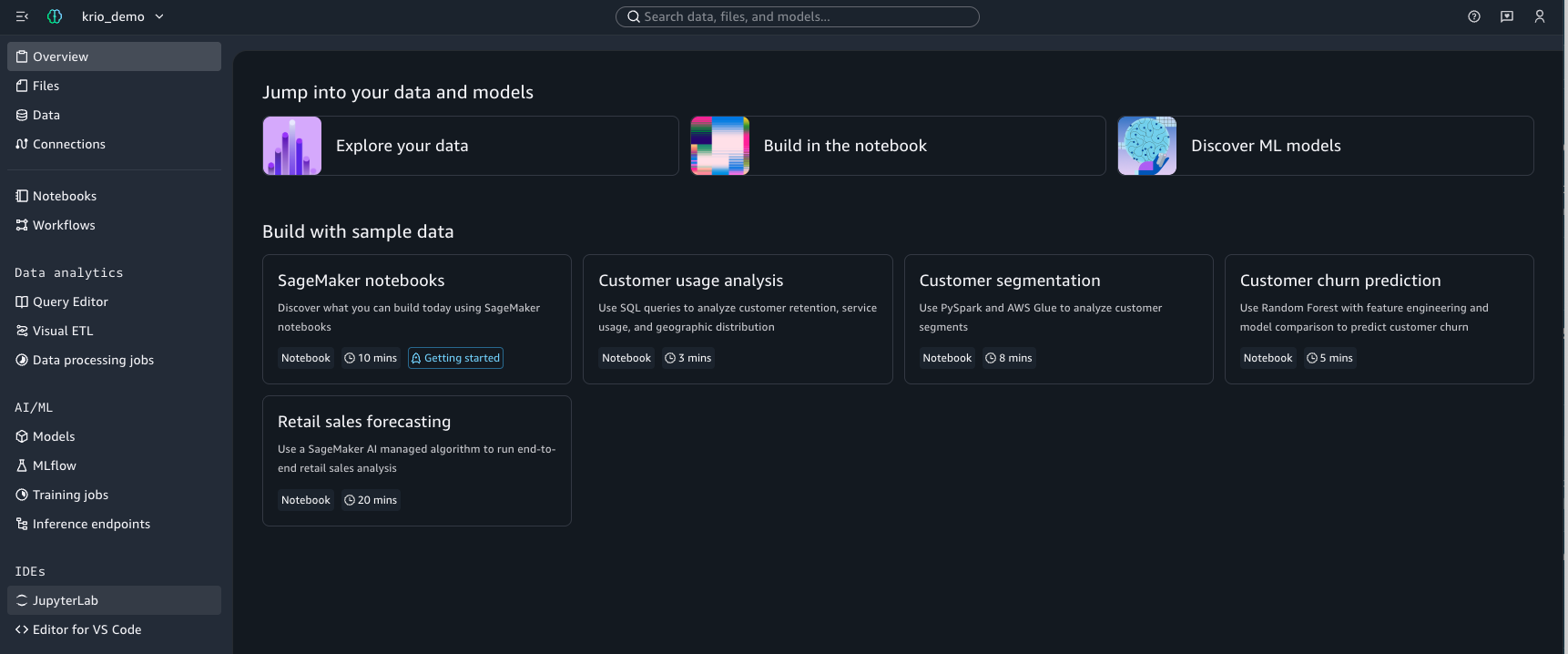
Figure 4 — SMUS project Spaces overview in the portal
Figure 5 — Configure Space dialog showing instance type selection
Figure 6 — Enabling Remote Access on a Space with 8 GiB or more
Connecting your editor to your SageMaker Space
There are two ways to connect: directly from the SageMaker Unified Studio portal, or from your local IDE using the AWS Toolkit.
Method 1: Connect from the SageMaker Unified Studio portal
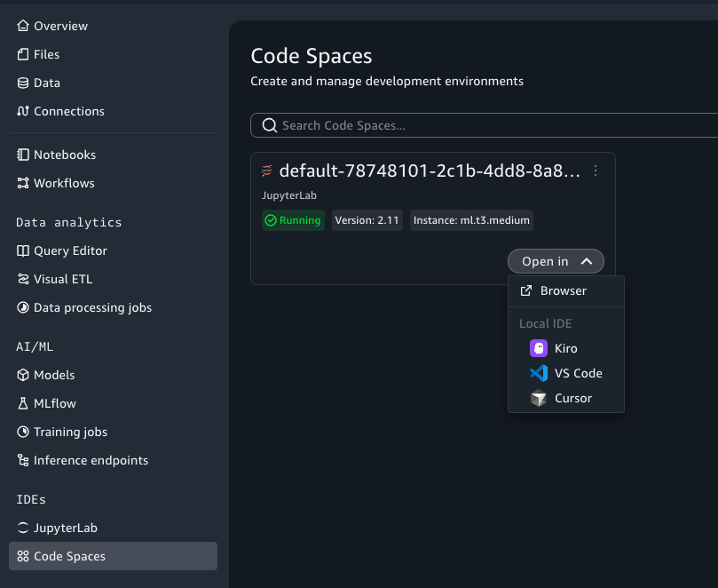
To launch your IDE directly from the portal, navigate to your project’s Code Spaces page, find your Space, and choose Open in to select your editor (Kiro, VS Code, or Cursor):
Figure 7 — Open in Local IDE from the Code Spaces list
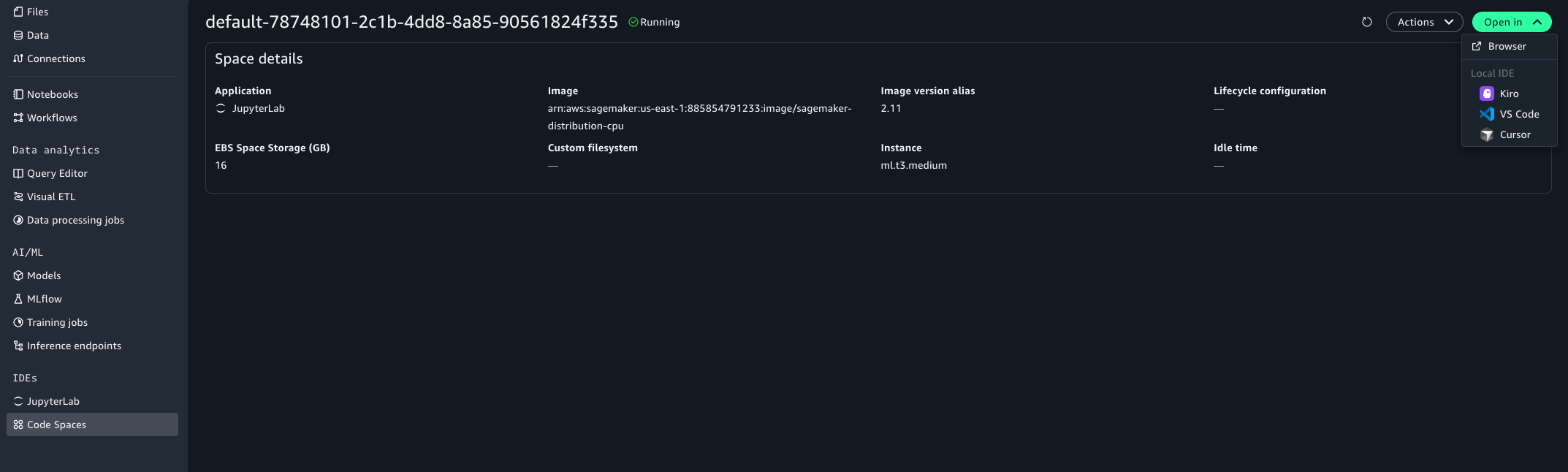
You can also launch from within a Space’s details page:
Figure 8 — Open in Local IDE from the Space details page
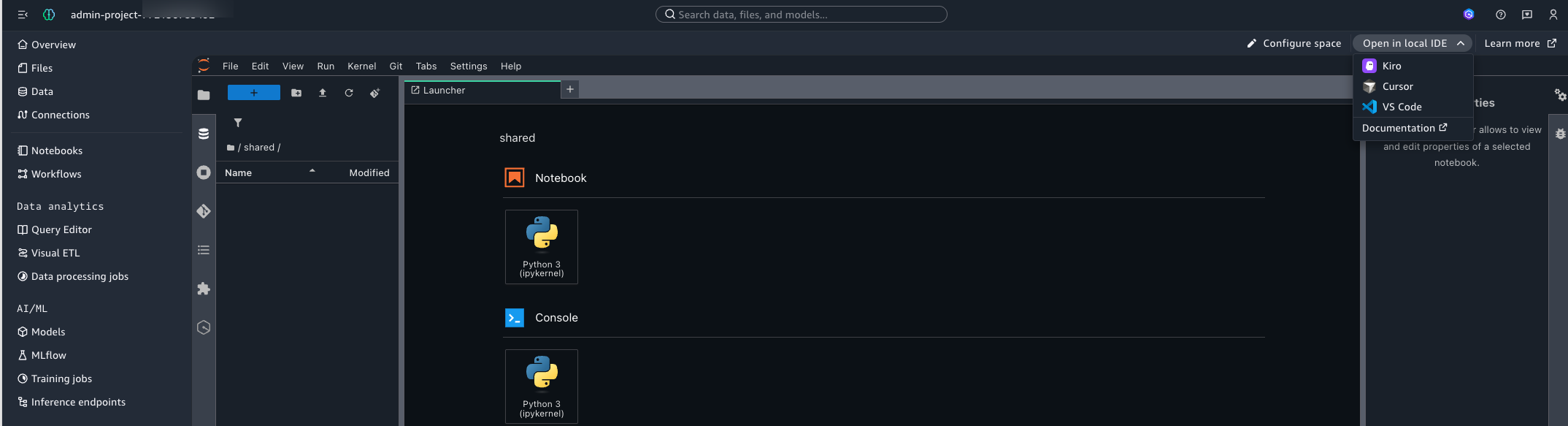
Or from within the JupyterLab or Code Editor browser environment:
Figure 9 — Open in Local IDE from JupyterLab
Your browser will prompt you to allow opening the IDE. Confirm, and the editor launches with an SSH connection to your Space already established via the AWS Toolkit. No additional configuration is typically required.
Method 2: Connect from your IDE via the AWS Toolkit
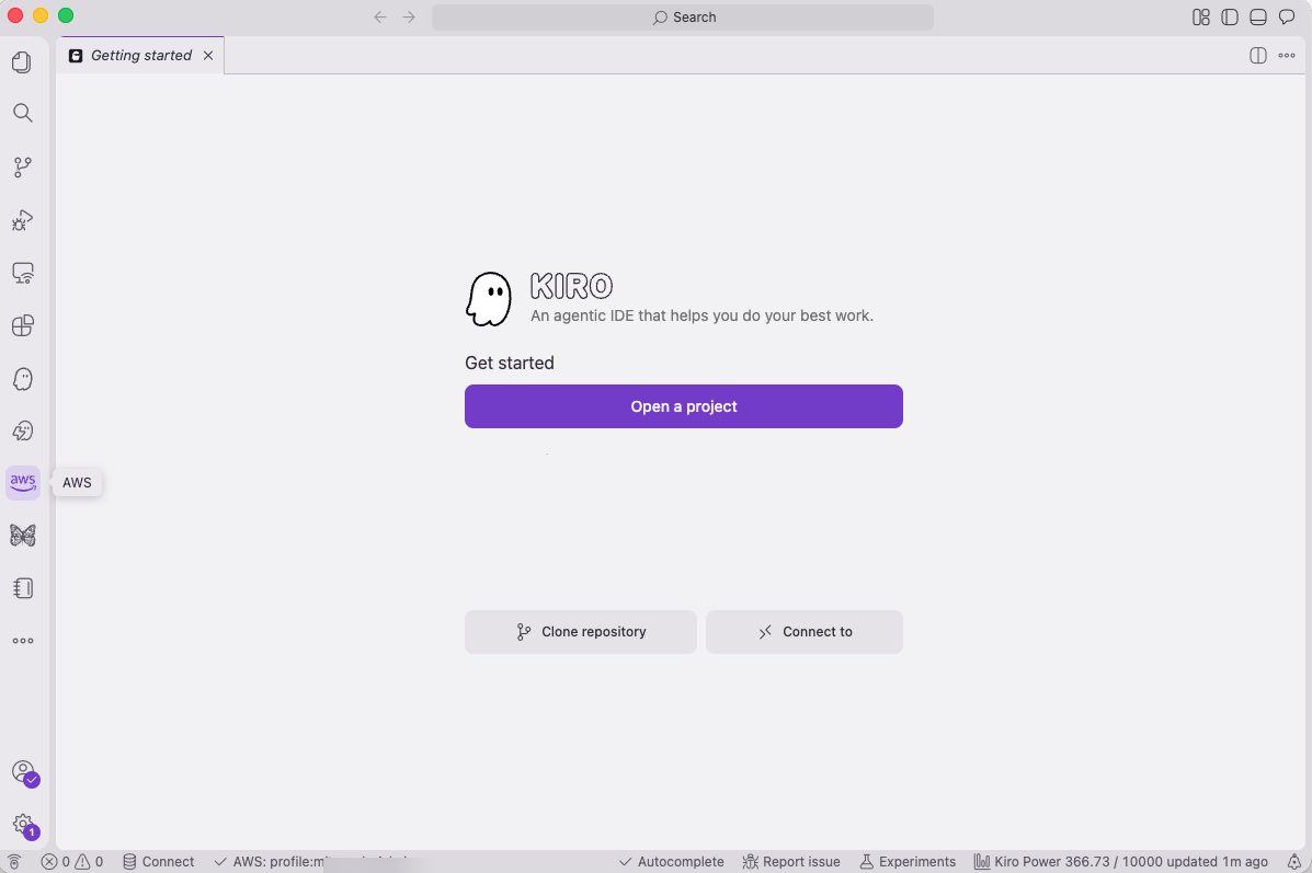
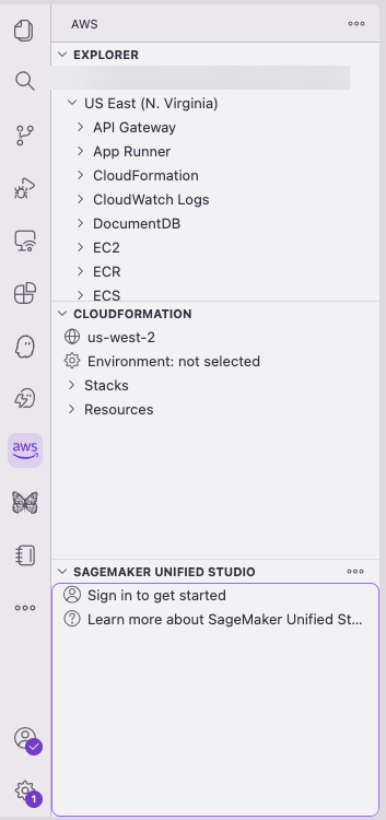
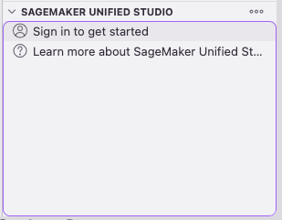
Open your editor on your local machine. Then, in the AWS Toolkit panel, choose Sign in. Authenticate with your IAM Identity Center or IAM credentials, the same identity you use to access SageMaker Unified Studio in the browser. The following screenshots show Kiro, but the steps are the same in VS Code and Cursor. Figure 10 — AWS Toolkit button in Kiro
Figure 11 — AWS Toolkit panel expanded
Figure 12 — AWS Toolkit Sign in dialog
Choose your AWS profile. You must have a profile configured in the AWS CLI with the correct account and AWS Region set.
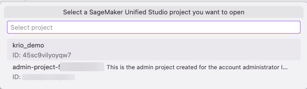
In the Toolkit panel, browse your SageMaker Unified Studio domains and projects. Select the project that you want to work in.
Figure 13 — Browsing SMUS domains and projects in Kiro
Important: The credentials that you use in the AWS Toolkit must match the identity that you use in the SageMaker Unified Studio portal. The Toolkit validates that your identity has access to the Space.
AI steering: How SageMaker Unified Studio pre-seeds AI context
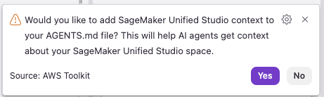
The real value of the feature comes from what you don’t need to do. When connected to Kiro SageMaker Unified Studio automatically generates steering files that guide your AI assistant with project context, so you can focus on building analytics rather than configuring connections. When you open a SageMaker Unified Studio project, SageMaker Unified Studio presents a prompt to create steering files: an AGENTS.md file that references a newly created smus-context.md. These files provide context about your project environment, such as project configuration, environment details, and utilities for discovering your data catalog and project structure. Kiro detects and applies these files automatically; in other editors, you can reference them as context for your AI features.
Figure 14 — SMUS popup offering to create steering files
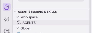
Figure 15 — Generated AGENTS.md and smus-context.md steering files
Without these steering files, your AI assistant would need several back-and-forth prompts to discover what data you have and how to access it. With them, the assistant understands your project from the first prompt: how to discover your databases, how your environment is configured, and what tools are available. The steering files also help properly configure MCP servers, which you set up in the next section.
Exploring your project
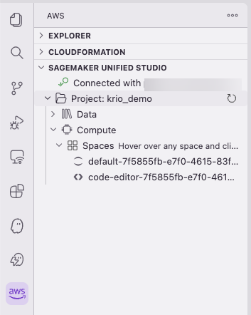
After you’re connected, the project structure expands into Data and Compute sections in the sidebar, as it would in the SageMaker Unified Studio portal.
Figure 16 — Project Data and Compute sections in the Kiro sidebar
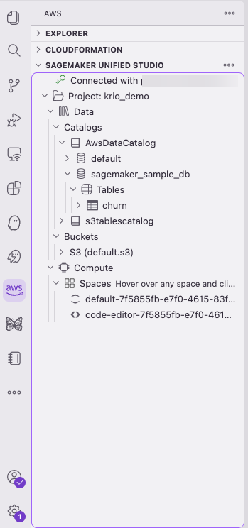
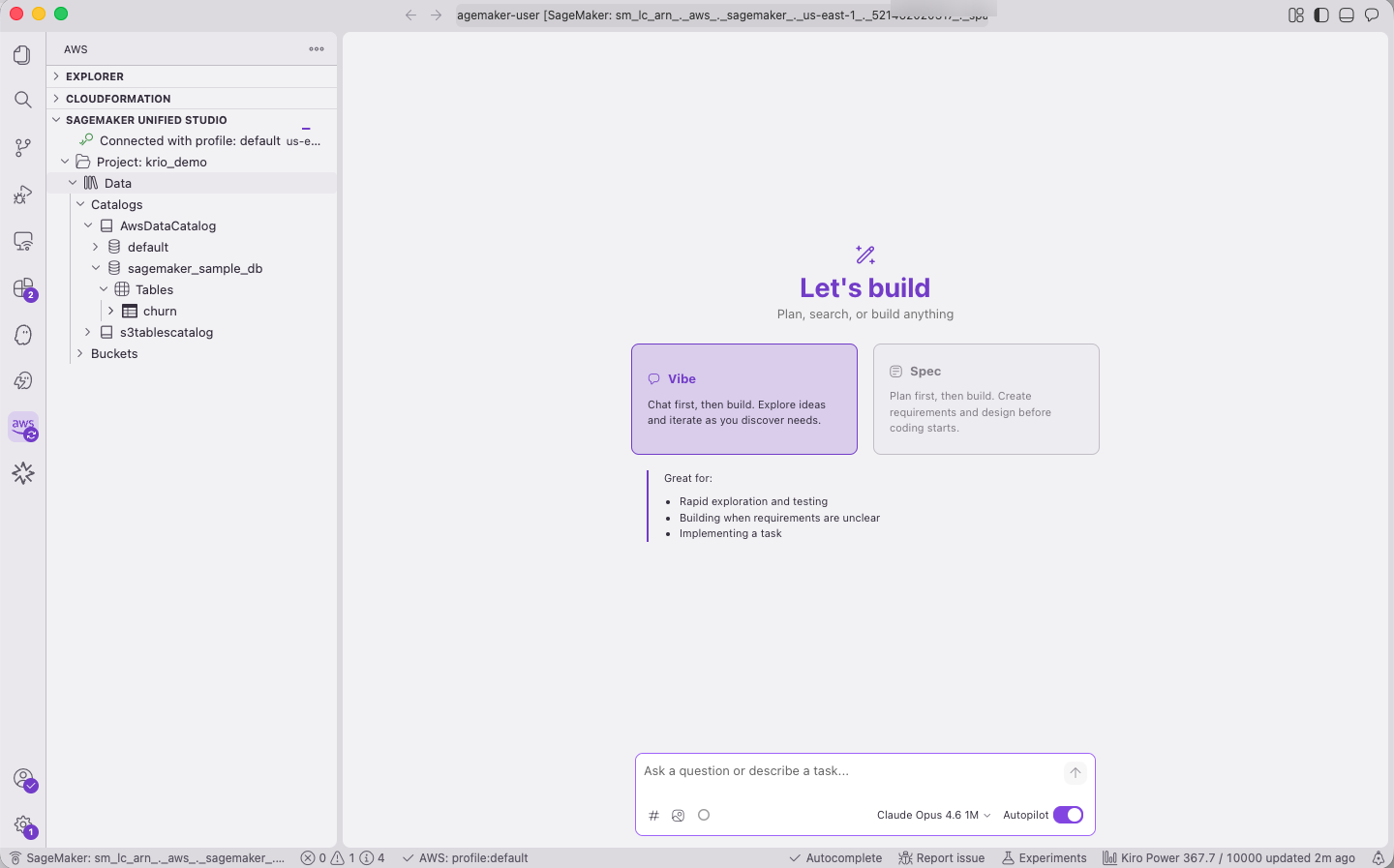
You can explore your data catalog and S3 buckets directly from the sidebar:
Figure 17 — Exploring the data catalog and S3 buckets from the sidebar
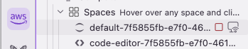
You can also remote into a compatible Space for direct development. Hover over a Space and select the remote icon on the right:
Figure 18 — Remote connection icon on a compatible Space
After a moment, the Space opens in a new Kiro window:
Figure 19 — Space opened in a new Kiro window
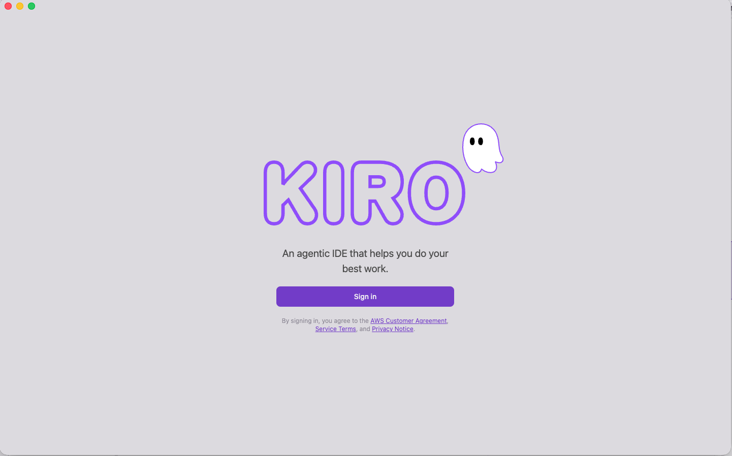
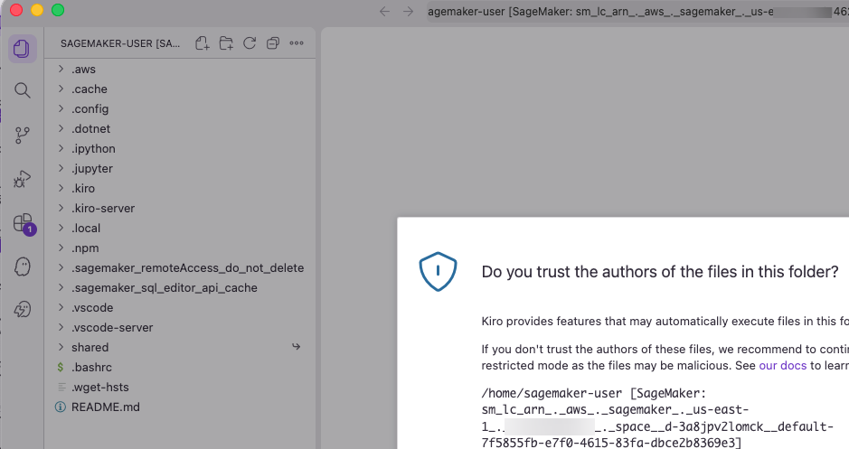
You must sign in again, and then trust the authors of the files in the Space:
Figure 20 — Trust authors dialog for the Space files
You’re now connected to your Space. The Toolkit works on the Space the way it does locally, except the resources are scoped to the project’s permissions.
Figure 21 — Connected to the SMUS Space with the Toolkit active
Setting up MCP servers
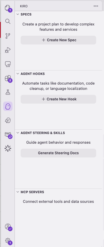
Before you can use AI-assisted development effectively, you must give Kiro access to your data services through Model Context Protocol (MCP) servers. MCP servers extend the Kiro agent with tools: the ability to query catalogs, run SQL, manage credentials, and more.
Out of the box, Kiro has no MCP servers configured:
Figure 22 — Kiro MCP servers panel with no servers configured
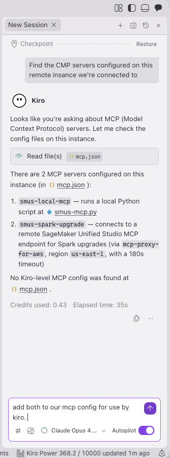
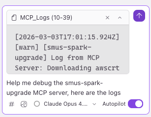
Prompt Kiro to find and configure the MCP servers that ship pre-installed on your SageMaker Space. Using the steering file context, Kiro located the servers and generated the configuration. If a server fails to connect, select the failed entry and Kiro will suggest fixes. You might need additional prompts to get the smus_spark_upgrade server (a pre-installed MCP server for managing Spark session upgrades) working correctly.
Figure 23 — Kiro discovering and configuring SMUS MCP servers
Figure 24 — MCP servers after iterating on configuration fixes
For more deterministic results, you can also configure the MCP servers manually. Here is a sample configuration:
Note: Your MCP configuration might vary depending on your SageMaker Unified Studio environment. Use the preceding configuration as a starting point and let your editor adjust if a server fails to connect.
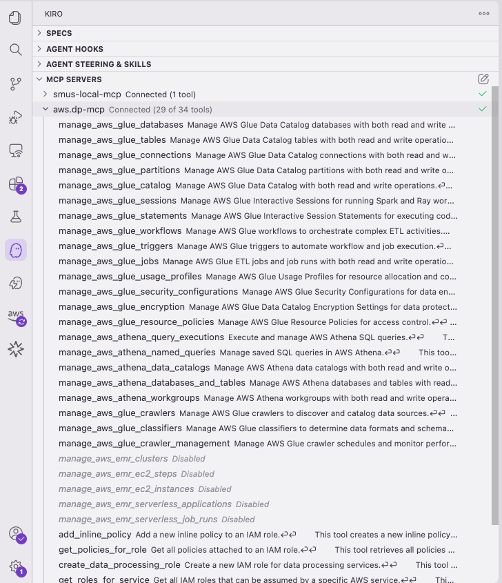
Next, add the AWS Data Processing MCP server to get catalog information and Athena query capabilities. This isn’t strictly required (Kiro can use Python or AWS CLI for the same tasks), but it gives the agent native tools for catalog and query operations.
Figure 25 — AWS Data Processing MCP server tools with Amazon EMR tools disabled
You can list the tools that each MCP server provides. Because the AWS Data Processing MCP server includes tools for many services, we recommend disabling tools that you don’t need for a given project to save model context. For this walkthrough, disable the Amazon EMR tools to focus on AWS Glue and Amazon Athena.
Exploring data with notebooks
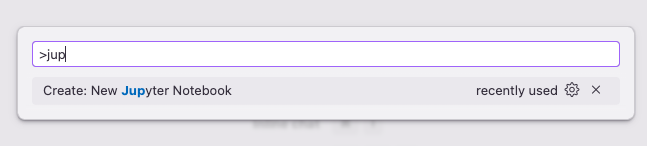
Kiro supports Jupyter notebooks in your SageMaker Space with the same language and connection selectors that you would find in SageMaker JupyterLab or Code Editor. Open the command palette (Cmd+Shift+P) and create a new Jupyter notebook:
Figure 26 — Command palette to create a new Jupyter notebook
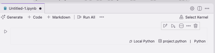
Figure 27 — New Jupyter notebook opened in Kiro with language and connection selectors in a notebook cell
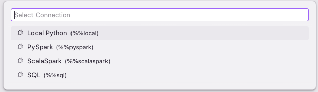
As in SageMaker JupyterLab, you get language and connection selectors in the bottom right of each cell. Choose the connection selector to see your available connections:
Figure 28 — SageMaker connection selector
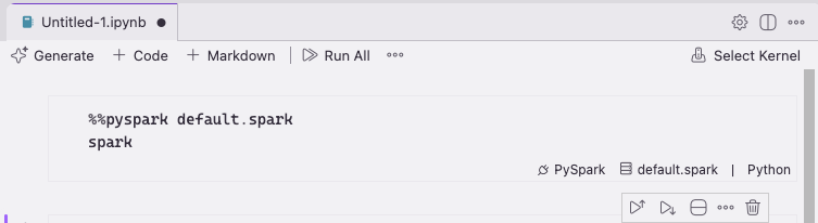
Select PySpark to fill in the magic commands for your cell. Write your code (in this case, enter spark and press Shift+Enter) to verify the session starts:
Figure 29 — PySpark magic command and spark verification code
Figure 30 — Running the PySpark cell
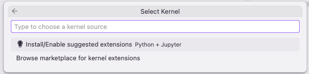
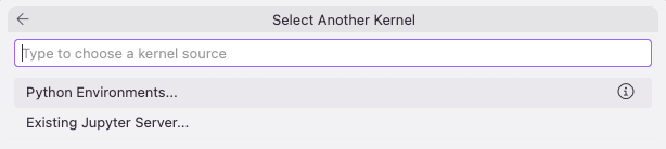
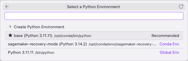
If this is your first time using Jupyter with Kiro, you’re prompted to install the Jupyter extension. After it’s installed, select the kernel from Python Environments → Base:
Figure 31 — Jupyter kernel selection prompt
Figure 32 — Selecting the Python kernel from the Base environment
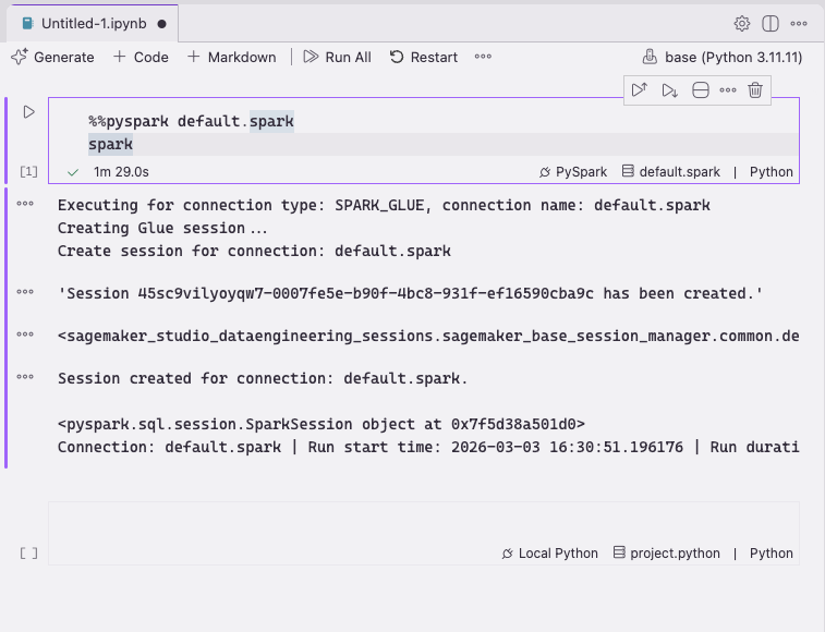
Re-run your cell. After a few moments, AWS Glue provisions a PySpark session:
Figure 33 — AWS Glue provisioning a PySpark session in a Jupyter notebook in Kiro
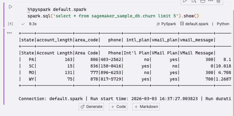
You see results the way you would in JupyterLab in the SageMaker Unified Studio portal:
Figure 34 — PySpark code running in a Jupyter notebook in Kiro
The notebook generate button
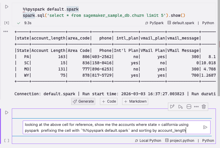
You will notice a Generate button underneath notebook cells. Let’s test it with a simple prompt:
looking at the above cell for reference, show me the accounts where state = california
using pyspark prefixing the cell with `%%pyspark default.spark` and sorting by
account_length
Figure 35 — Using the Generate button with a natural language prompt
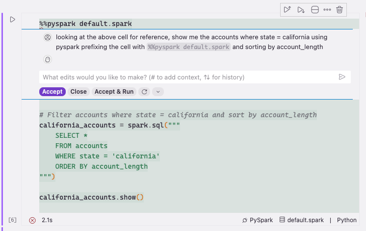
Figure 36 — Generated PySpark code from the prompt
This prompt builder, like other notebook generation features, doesn’t have good context on the surrounding cells. You must be explicit about what you want because it won’t read other code or cells as input.
While the Kiro notebook generate button works for straightforward edits, for serious code generation, we recommend that you use Kiro agent mode. This mode has full project and SageMaker context, as demonstrated in the “See it in action” walkthrough earlier in this post.
What’s happening under the hood
When you connect your editor to a SageMaker Unified Studio Space, the AWS Toolkit extension establishes a secure SSH tunnel between your local IDE and your cloud-based Space.
Key details:
SSH tunnel. The connection is managed entirely by the AWS Toolkit (v4.1.0+) or VS Code’s built-in SSH extension. No separate Remote SSH extension is needed; the capability is built in.
File system access. Your editor sees the Space’s persistent storage at /home/sagemaker-user/, including shared project files and notebooks or scripts you create.
SageMaker Unified Studio steering context. The integration generates AGENTS.md and smus-context.md files that provide your AI assistant with context about your project environment and utilities for understanding your data. This is what makes the assistant effective from the first prompt.
MCP server integration. MCP servers like smus_local (for project metadata and environment utilities) and aws-dataprocessing (for AWS Glue Data Catalog and Amazon Athena) extend your editor’s AI with direct access to your data services. Your own MCP servers will be equally valuable here.
Credential flow. The Toolkit uses your existing AWS identity (IAM Identity Center or IAM) to authenticate to the Space. No separate SSH keys to manage. The aws_context_provider tool from the smus_local MCP server handles credential discovery for agent operations.
Best practices
To work effectively with your IDE and SageMaker Unified Studio:
Explore your data before building. Start every session by asking your AI assistant to discover your catalog, sample your data, and understand the schema. This single step helps reduce the most common source of errors in AI-assisted data work: the LLM making assumptions about data it has not seen. See the “See it in action” walkthrough earlier in this post for a concrete example of the difference this makes.
Use the SageMaker Unified Studio steering files. When prompted to create AGENTS.md and smus-context.md, accept. These files are the foundation that makes everything else work: environment context, MCP server configuration, and project understanding. Without them, your AI assistant starts from zero on every prompt. Kiro detects these automatically; in other editors, add them as context.
Disable unused MCP tools. The AWS Data Processing MCP server includes tools for AWS Glue, Amazon EMR, Amazon Athena, and more. Disable the services that you’re not using for a given project to save model context and reduce noise.
Be specific in your prompts. The more detail you give your AI (column names, query patterns you prefer, output formats), the closer the first pass will be. “Run data quality evaluation using Athena SQL” gets you better code than “check my data.”
Always test interactively first. Whether in notebooks or the terminal, validate code before deploying it. AI agents can iterate quickly, but catching issues in an interactive session is faster than debugging a failed AWS Glue job. Athena PySpark and the SageMaker sqlutils and sparkutils packages are great for this.
Stop your Space when idle. Your Space runs on compute (the same instance types as Code Editor and JupyterLab). If idle, the Space will terminate after 60 minutes and close your remote connection. Close the remote window and reconnect to continue.
Things to know
Notebook agent mode. For notebook-heavy analytics workflows where you want agentic AI to generate and run cells directly, SageMaker Notebooks with Data Agent in SageMaker Unified Studio is the recommended option today. Current notebook support in local editors covers editing, running, and generating code in individual cells.
MCP setup takes iteration. Configuring MCP servers may require iteration, especially for servers with complex authentication. Many AI-enabled editors can self-correct when a server fails. For more deterministic results, use the preceding MCP configuration JSON as a starting point rather than relying solely on auto-discovery.
CLI preference. AI agents often prefer the AWS CLI and bash even when MCP tools are available. This doesn’t affect outcomes, but you can steer your assistant toward MCP tools using a steering document if you prefer consistency.
Security and governance boundaries
A core benefit of this integration is that your existing security and governance controls remain enforced. Your editor connects to your SageMaker Space through a secure SSH tunnel managed by the AWS Toolkit. It does not bypass your organization’s access controls. Data access is governed by the same AWS Lake Formation permissions and IAM Identity Center authentication that apply when you work in the SageMaker Unified Studio portal directly. Your project-level permissions, database grants, and column-level security policies apply consistently whether a query originates from an AI agent, a notebook cell, or the SageMaker console. Data access is governed by the boundaries you define in your SageMaker Unified Studio domain and project configuration.
Clean up
To avoid ongoing charges from billable resources (SageMaker Space compute charges per hour, AWS Glue sessions charge per DPU-hour, Amazon Athena queries charge per TB scanned):
Stop your Space – In the SageMaker Unified Studio portal, navigate to your project’s Spaces and stop the Space you used for this walkthrough.
Disconnect: Close the remote connection in your editor (File → Close Remote Connection).
Verify AWS Glue sessions are terminated – If you ran PySpark queries during this walkthrough, verify that the sessions are stopped. In the SageMaker Unified Studio portal, navigate to Data processing and confirm no active AWS Glue sessions remain. Sessions auto-terminate when the Space stops, but verify to avoid unexpected charges.
Delete demo resources (optional) – File deletion is permanent and cannot be undone. Back up any work that you want to retain before proceeding. If you created scripts or files during this walkthrough that you no longer need, delete them from /home/sagemaker-user/. For example, delete any test notebooks, Python scripts, or generated data files. The sample sagemaker_sample_db.churn dataset is read-only and doesn’t need cleanup.
Conclusion
This post showed what happens when agentic AI meets governed data, and walked through how to set it up yourself.
Three key insights emerged from this hands-on experience:
SageMaker Unified Studio steering files transform the developer experience. Your AI assistant is project-aware from the first prompt, understanding your environment and available data without manual setup.
MCP servers bridge “AI that writes code” with “AI that queries your data”. The smus_local and aws-dataprocessing servers are essential for effective agentic data work.
The “explore first” pattern pays immediate dividends. When your AI assistant understands your data before writing code, it makes smarter engine choices and produces correct analytics on the first pass.
This integration brings together two capabilities that are stronger together: your IDE handles the AI-assisted coding and iteration, while SageMaker Unified Studio handles data governance, access control, and compute management. You get the productivity of an agentic AI coding assistant without compromising on the controls your organization requires.
AWS Glue is a serverless data integration service that makes it simple to discover, prepare, move, and integrate data from multiple sources for analytics, machine learning (ML), and application development. Today, AWS Glue processes customer jobs using either Apache Spark’s distributed processing engine for large workloads or Python’s single-node processing engine for smaller workloads. Customers like Python for its ease of use and rich collection of built-in data-processing libraries but might find it difficult for customers to scale Python beyond a single compute node. This limitation makes it difficult for customers to process large datasets. Customers want a solution that allows them to continue using familiar Python tools and AWS Glue jobs on data sets of all sizes, even those that can’t fit on a single instance.
We are happy to announce the release of a new AWS Glue job type: Ray. Ray is an open-source unified compute framework that makes it simple to scale AI and Python workloads. Ray started as an open-source project at RISELab in UC Berkeley. If your application is written in Python, you can scale it with Ray in a distributed cluster in a multi-node environment. Ray is Python native and you can combine it with the AWS SDK for pandas to prepare, integrate and transform your data for running your data analytics and ML workloads in combination.
This post provides an introduction to AWS Glue for Ray and shows you how to start using Ray to distribute your Python workloads.
What is AWS Glue for Ray?
Customers like the serverless experience and fast start time offered by AWS Glue. With the introduction of Ray, we have ensured that you get the same experience. We have also ensured that you can use the AWS Glue job and AWS Glue interactive session primitives to access the Ray engine. AWS Glue jobs are fire-and-forget systems where customer submit their Ray code to the AWS Glue jobs API and AWS Glue automatically provisions the required compute resources and runs the job. AWS Glue interactive session APIs allow interactive exploration of the data for the purpose of job development. Regardless of the option used, you are only billed for the duration of the compute used. With AWS Glue for Ray, we are also introducing a new Graviton2 based worker (Z.2x) which offers 8 virtual CPUs and 64 GB of RAM.
AWS Glue for Ray consists of two major components:
Ray Dataset – The distributed data framework based on Apache Arrow
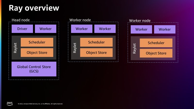
When running a Ray job, AWS Glue provisions the Ray cluster for you and runs these distributed Python jobs on a serverless auto-scaling infrastructure. The cluster in AWS Glue for Ray will consists of exactly one head node and one or more worker nodes.
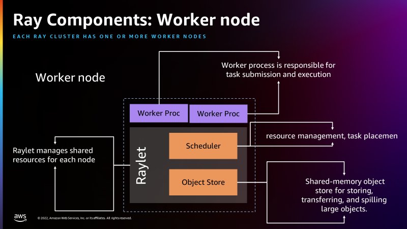
The head node is identical to the other worker nodes with the exception that it runs singleton processes for cluster management and the Ray driver process. The driver is a special worker process in the head node that runs the top-level application in Python that starts the Ray job. The worker node has processes that are responsible for submitting and running tasks.
The following figure provides a simple introduction to the Ray architecture. The architecture illustrates how Ray is able to schedule jobs through processes called Raylets. The Raylet manages the shared resources on each node and is shared between the concurrently running jobs. For more information on how Ray works, see Ray.io.
The following figure shows the components of the worker node and the shared-memory object store:
There is a Global Control Store in the head node that can treat each separate machine as nodes, similar to how Apache Spark treats workers as nodes. The following figure shows the components of the head node and the Global Control Store managing the cluster-level metadata.
AWS Glue for Ray comes included with Ray Core, Ray Dataset, Modin (distributed pandas) and the AWS SDK for pandas (on Modin) for seamless distributed integration into other AWS services. Ray Core is the foundation of Ray and the basic framework for distributing Python functions and classes. Ray Dataset is a distributed data framework based on Apache Arrow and is most closely analogous to a dataframe in Apache Spark. Modin is a library designed to distribute pandas applications across a Ray cluster without any modification and is compatible with data in Ray Datasets. The included AWS SDK for pandas (formerly AWS Data Wrangler) is an abstraction layer on top of Modin to allow for the creation of pandas dataframes from (and writing to) many AWS sources such as Amazon Simple Storage Service (Amazon S3), Amazon Redshift, Amazon DynamoDB, Amazon OpenSearch Service, and others.
You can also install your own ARM compatible Python libraries via pip, either through Ray’s environmental configuration in @ray.remote or via --additional-python-modules.
To learn more about Ray, please visit the GitHub repo.
Why use AWS Glue for Ray?
Many of us start our data journey on AWS with Python, looking to prepare data for ML and data science, and move data at scale with AWS APIs and Boto3. Ray allows you to bring those familiar skills, paradigms, frameworks and libraries to AWS Glue and make them scale to handle massive datasets with minimal code changes. You can use the same data processing tools you currently have (such as Python libraries for data cleansing, computation, and ML) on datasets of all sizes. AWS Glue for Ray enables the distributed run of your Python scripts over multi-node clusters.
AWS Glue for Ray is designed for the following:
Task parallel applications (for example, when you want to apply multiple transforms in parallel)
Speeding up your Python workload as well as using Python native libraries.
Running the same workload across hundreds of data sources.
ML ingestion and parallel batch inference on data
Solution overview
For this post, you will use the Parquet Amazon Customer Reviews Dataset stored in the public S3 bucket. The objective is to perform transformations using the Ray dataset and then write it back to Amazon S3 in the Parquet file format.
Configure Amazon S3
The first step is to create an Amazon S3 bucket to store the transformed Parquet dataset as the end result.
For Bucket name, enter a name for your Amazon S3 bucket.
Choose Create.
Set up a Jupyter notebook with an AWS Glue interactive session
For our development environment, we use a Jupyter notebook to run the code.
You’re required to install the AWS Glue interactive sessions locally or run interactive sessions with an AWS Glue Studio notebook. Using AWS Glue Interactive sessions will help you follow and run the series of demonstration steps.
This section walks you through several notebook paragraphs on how to use AWS Glue for Ray. In this exercise, we look at the customer reviews from the Amazon Customer Review Parquet dataset, perform some Ray transformations, and write the results to Amazon S3 in a Parquet format.
On Jupyter console, under New, choose Glue Python.
Signify you want to use Ray as the engine by using the %glue_ray magic.
Import the Ray library along with additional Python libraries:
%glue_ray

import ray
import pandas
import pyarrow
from ray import data
import time
from ray.data import ActorPoolStrategy
Initialize a Ray Cluster with AWS Glue.
ray.init('auto')
Next, we read a single partition from the dataset, which is Parquet file format:
start = time.time()
ds = ray.data.read_parquet("s3://amazon-reviews-pds/parquet/product_category=Wireless/")
end = time.time()
print(f"Reading the data to dataframe: {end - start} seconds")
Parquet files store the number of rows per file in the metadata, so we can get the total number of records in ds without performing a full data read:
ds.count()
Next , we can check the schema of this dataset. We don’t have to read the actual data to get the schema; we can read it from the metadata:
ds.schema()
We can check the total size in bytes for the full Ray dataset:
#calculate the size in bytes of the full dataset,  Note that for Parquet files, this size-in-bytes will be pulled from the Parquet
#  metadata (not triggering a data read).
ds.size_bytes()
We can see a sample record from the Ray dataset:
#Show sample records from the underlying Parquet dataset
start = time.time()
ds.show(1)
end = time.time()
print(f"Time taken to show the data from dataframe : {end - start} seconds")
Applying dataset transformations with Ray
There are primarily two types of transformations that can be applied to Ray datasets:
One-to-One transformations – Each input block will contributes to only one output block, such as add_column(), map_batches() and drop_column() , and so on.
All-to-All transformations – Input blocks can contribute to multiple output blocks such as sort() and groupby(), and so on.
In the next series of steps we will apply some of these transformations on our resultant Ray datasets from the previous section.
We can add a new column and check the schema to verify the newly added column, followed by retrieving a sample record. This transformation is only available for the datasets that can be converted to pandas format.
# Add the given new column to the dataset and show the sample record after adding a new column

start = time.time()
ds = ds.add_column( "helpful_votes_ratio", lambda df: df["helpful_votes"] / df["total_votes"])
end = time.time()
print(f"Time taken to Add a new columns : {end - start} seconds")
ds.show(1)
Let’s drop a few columns we don’t need using a drop_columns transformation and then check the schema to verify if those columns are dropped from the Ray dataset:
# Dropping few columns from the underlying Dataset
start = time.time()
ds = ds.drop_columns(["review_body", "vine", "product_parent", "verified_purchase", "review_headline"])
end = time.time()
print(f"Time taken to drop a few columns : {end - start} seconds")
ds.schema()
Ray datasets have built-in transformations such as sorting the dataset by the specified key column or key function.
Next, we apply the sort transformation using one of the columns present in the dataset (total_votes):
#Sort the dataset by total votes
start = time.time()
ds =ds.sort("total_votes")
end = time.time()
print(f"Time taken for sort operation  : {end - start} seconds")
ds.show(3)
Next, we will create a Python UDF function that allows you to write customized business logic in transformations. In our UDF we have written a logic to find out the products that are rated low (i.e. total votes less than 100).We create a UDF as a function on pandas DataFrame batches. For the supported input batch formats, see the UDF Input Batch Format. We also demonstrate using map_batches() which applies the given function to the batches of records of this dataset. Map_batches() uses the default compute strategy (tasks), which helps distribute the data processing to multiple Ray workers, which are used to run tasks. For more information on a map_batches() transformation, please see the following documentation.
# UDF as a function on pandas DataFrame - To Find products with total_votes < 100
def low_rated_products(df: pandas.DataFrame) -> pandas.DataFrame:
    return df[(df["total_votes"] < 100)]

#Calculate the number of products which are rated low in terms of low votes i.e. less than 100
# This technique is called Batch inference processing with Ray tasks (the default compute strategy).
ds = ds.map_batches(low_rated_products)

#See sample records for the products which are rated low in terms of low votes i.e. less than 100
ds.show(1)
#Count total number of products which are rated low
ds.count()
If you have complex transformations that require more resources for data processing, we recommend utilizing Ray actors using additional configurations with applicable transformations. We have demonstrated with map_batches() below:
# Batch inference processing with Ray actors. Autoscale the actors between 2 and 4.

class LowRatedProducts:
    def __init__(self):
        self._model = low_rated_products

    def __call__(self, batch: pandas.DataFrame) -> pandas.DataFrame:
        return self._model(batch)

start = time.time()
predicted = ds.map_batches(
    LowRatedProducts, compute=ActorPoolStrategy(2, 4), batch_size=4)
end = time.time()
Next, before writing the final resultant Ray dataset we will apply map_batches() transformations to filter out the customer reviews data where the total votes for a given product is greater than 0 and the reviews belongs to the “US” marketplace only. Using map_batches() for the filter operation is better in terms of performance in comparison to filter() transformation.
# Filter our records with total_votes == 0
ds = ds.map_batches(lambda df: df[df["total_votes"] > 0])

# Filter and select records with marketplace equals US only
ds = ds.map_batches(lambda df: df[df["marketplace"] == 'US'])

ds.count()
Finally, we write the resultant data to the S3 bucket you created in a Parquet file format. You can use different dataset APIs available, such as write_csv() or write_json() for different file formats. Additionally, you can convert the resultant dataset to another DataFrame type such as Mars, Modin or pandas.
To avoid incurring future charges, delete the Amazon S3 bucket and Jupyter notebook.
On the Amazon S3 console, choose Buckets.
Choose the bucket you created.
Choose Empty and enter your bucket name.
Choose Confirm.
Choose Delete and enter your bucket name.
Choose Delete bucket.
On the AWS Glue console, choose Interactive Sessions
Choose the interactive session you created.
Choose Delete to remove the interactive session.
Conclusion
In this post, we demonstrated how you can use AWS Glue for Ray to run your Python code in a distributed environment. You can now run your data and ML applications in a multi-node environment.
Refer to the Ray documentation for additional information and use cases.
About the authors
Zach Mitchell is a Sr. Big Data Architect. He works within the product team to enhance understanding between product engineers and their customers while guiding customers through their journey to develop data lakes and other data solutions on AWS analytics services.
Ishan Gaur works as Sr. Big Data Cloud Engineer ( ETL ) specialized in AWS Glue. He’s passionate about helping customers build out scalable distributed ETL workloads and implement scalable data processing and analytics pipelines on AWS. When not at work, Ishan likes to cook, travel with his family, or listen to music.
Derek Liu is a Solutions Architect on the Enterprise team based out of Vancouver, BC. He is part of the AWS Analytics field community and enjoys helping customers solve big data challenges through AWS analytic services.
Kinshuk Pahare is a Principal Product Manager on AWS Glue.
Interactive Sessions for Jupyter is a new notebook interface in the AWS Glue serverless Spark environment. Starting in seconds and automatically stopping compute when idle, interactive sessions provide an on-demand, highly-scalable, serverless Spark backend to Jupyter notebooks and Jupyter-based IDEs such as Jupyter Lab, Microsoft Visual Studio Code, JetBrains PyCharm, and more. Interactive sessions replace AWS Glue development endpoints for interactive job development with AWS Glue and offers the following benefits:
No clusters to provision or manage
No idle clusters to pay for
No up-front configuration required
No resource contention for the same development environment
Easy installation and usage
The exact same serverless Spark runtime and platform as AWS Glue extract, transform, and load (ETL) jobs
Getting started with interactive sessions for Jupyter
Installing interactive sessions is simple and only takes a few terminal commands. After you install it, you can run interactive sessions anytime within seconds of deciding to run. In the following sections, we walk you through installation on macOS and getting started in Jupyter.
Install AWS Glue interactive sessions on macOS and Linux
To install AWS Glue interactive sessions, complete the following steps:
Open a terminal and run the following to install and upgrade Jupyter, Boto3, and AWS Glue interactive sessions from PyPi. If desired, you can install Jupyter Lab instead of Jupyter.
To validate your install, run the following command:
jupyter kernelspec list
In the output, you should see both the AWS Glue PySpark and the AWS Glue Spark kernels listed alongside the default Python3 kernel. It should look something like the following:
Available kernels:
  Python3		~/.venv/share/jupyter/kernels/python3
  glue_pyspark    /usr/local/share/jupyter/kernels/glue_pyspark
  glue_spark      /usr/local/share/jupyter/kernels/glue_spark
Choose and prepare IAM principals
Interactive sessions use two AWS Identity and Access Management (IAM) principals (user or role) to function. The first is used to call the interactive sessions APIs and is likely the same user or role that you use with the AWS CLI. The second is GlueServiceRole, the role that AWS Glue assumes to run your session. This is the same role as AWS Glue jobs; if you’re developing a job with your notebook, you should use the same role for both interactive sessions and the job you create.
Prepare the client user or role
In the case of local development, the first role is already configured if you can run the AWS CLI. If you can’t run the AWS CLI, follow these steps for setting up. If you often use the AWS CLI or Boto3 to interact with AWS Glue and have full AWS Glue permissions, you can likely skip this step.
To validate this first user or role is set up, open a new terminal window and run the following code:
aws sts get-caller-identity
You should see a response like the following. If not, you may not have permissions to call AWS Security Token Service (AWS STS), or you don’t have the AWS CLI set up properly. If you simply get access denied calling AWS STS, you may continue if you know your user or role and its needed permissions.
Ensure your IAM user or role can call the AWS Glue interactive sessions APIs by attaching the AWSGlueConsoleFullAccess managed IAM policy to your role.
If your caller identity returned a user, run the following:
aws iam attach-user-policy --role-name <myIAMUser> --policy-arn arn:aws:iam::aws:policy/AWSGlueConsoleFullAccess
If your caller identity returned a role, run the following:
aws iam attach-role-policy --role-name, --policy-arn arn:aws:iam::aws:policy/AWSGlueConsoleFullAccess
Prepare the AWS Glue service role for interactive sessions
You can specify the second principal, GlueServiceRole, either in the notebook itself by using the %iam_role magic or stored alongside the AWS CLI config. If you have a role that you typically use with AWS Glue jobs, this will be that role. If you don’t have a role you use for AWS Glue jobs, refer to Setting up IAM permissions for AWS Glue to set one up.
To set this role as the default role for interactive sessions, edit the AWS CLI credentials file and add glue_role_arn to the profile you intend to use.
With a text editor, open ~/.aws/credentials. On Windows, use C:\Users\username\.aws\credentials.
Look for the profile you use for AWS Glue; if you don’t use a profile, you’re looking for [Default].
Add a line in the profile for the role you intend to use like, glue_role_arn=<AWSGlueServiceRole>.
I recommend adding a default Region to your profile if one is not specified already. You can do so by adding the line region=us-east-1, replacing us-east-1 with your desired Region. If you don’t add a Region to your profile, you’re required to specify the Region at the top of each notebook with the %region magic.When finished, your config should look something like the following:
To start Jupyter and your notebook, complete the following steps:
Run the following command in your terminal to open the Jupyter notebook in your browser:
jupyter notebook
Your browser should open and you’re presented with a page that looks like the following screenshot.
On the New menu, choose Glue PySpark.
A new tab opens with a blank Jupyter notebook using the AWS Glue PySpark kernel.
Configure your notebook with magics
AWS Glue interactive sessions are configured with Jupyter magics. Magics are small commands prefixed with % at the start of Jupyter cells that provide shortcuts to control the environment. In AWS Glue interactive sessions, magics are used for all configuration needs, including:
%region – Region
%profile – AWS CLI profile
%iam_role – IAM role for the AWS Glue service role
%worker_type – Worker type
%number_of_workers – Number of workers
%idle_timeout – How long to allow a session to idle before stopping it
%additional_python_modules – Python libraries to install from pip
Magics are placed at the beginning of your first cell, before your code, to configure AWS Glue. To discover all the magics of interactive sessions, run %help in a cell and a full list is printed. With the exception of %%sql, running a cell of only magics doesn’t start a session, but sets the configuration for the session that starts next when you run your first cell of code. For this post, we use three magics to configure AWS Glue with version 2.0 and two G.2X workers. Let’s enter the following magics into our first cell and run it:
%glue_version 2.0
%number_of_workers 2
%worker_type G.2X
%idle_tiemout 60


Welcome to the Glue Interactive Sessions Kernel
For more information on available magic commands, please type %help in any new cell.

Please view our Getting Started page to access the most up-to-date information on the Interactive Sessions kernel: https://docs.aws.amazon.com/glue/latest/dg/interactive-sessions.html
Setting Glue version to: 2.0
Previous number of workers: 5
Setting new number of workers to: 2
Previous worker type: G.1X
Setting new worker type to: G.2X
When you run magics, the output lets us know the values we’re changing along with their previous settings. Explicitly setting all your configuration in magics helps ensure consistent runs of your notebook every time and is recommended for production workloads.
Run your first code cell and author your AWS Glue notebook
Next, we run our first code cell. This is when a session is provisioned for use with this notebook. When interactive sessions are properly configured within an account, the session is completely isolated to this notebook. If you open another notebook in a new tab, it gets its own session on its own isolated compute. Run your code cell as follows:
from awsglue.context import GlueContext
from awsglue.job import Job
from awsglue.transforms import *
from awsglue.utils import getResolvedOptions
from pyspark.context import SparkContext

sc = SparkContext.getOrCreate()
glueContext = GlueContext(sc)
spark = glueContext.spark_session
job = Job(glueContext)

Authenticating with profile=default
glue_role_arn defined by user: arn:aws:iam::123456789123:role/AWSGlueServiceRoleForSessions
Attempting to use existing AssumeRole session credentials.
Trying to create a Glue session for the kernel.
Worker Type: G.2X
Number of Workers: 2
Session ID: 12345678-12fa-5315-a234-567890abcdef
Applying the following default arguments:
--glue_kernel_version 0.31
--enable-glue-datacatalog true
Waiting for session 12345678-12fa-5315-a234-567890abcdef to get into ready status...
Session 12345678-12fa-5315-a234-567890abcdef has been created
When you ran the first cell containing code, Jupyter invoked interactive sessions, provisioned an AWS Glue cluster, and sent the code to AWS Glue Spark. The notebook was given a session ID, as shown in the preceding code. We can also see the properties used to provision AWS Glue, including the IAM role that AWS Glue used to create the session, the number of workers and their type, and any other options that were passed as part of the creation.
Interactive sessions automatically initialize a Spark session as spark and SparkContext as sc; having Spark ready to go saves a lot of boilerplate code. However, if you want to convert your notebook to a job, spark and sc must be initialized and declared explicitly.
Work in the notebook
Now that we have a session up, let’s do some work. In this exercise, we look at population estimates from the AWS COVID-19 dataset, clean them up, and write the results a table.
This walkthrough uses data from the COVID-19 data lake.
To make the data from the AWS COVID-19 data lake available in the Data Catalog in your AWS account, create an AWS CloudFormation stack using the following template.
If you’re signed in to your AWS account, deploy the CloudFormation stack by clicking the following Launch stack button:
It fills out most of the stack creation form for you. All you need to do is choose Create stack. For instructions on creating a CloudFormation stack, see Get started.
When I’m working on a new data integration process, the first thing I often do is identify and preview the datasets I’m going to work on. If I don’t recall the exact location or table name, I typically open the AWS Glue console and search or browse for the table then return to my notebook to preview it. With interactive sessions, there is a quicker way to browse the Data Catalog. We can use the %%sql magic to show databases and tables without leaving the notebook. For this example, the population table I want in is the COVID-19 dataset but I don’t recall its exact name, so I use the %%sql magic to look it up:
%%sql
show tables in `covid-19`  # Remember, dashes in names must be escaped with backticks.

+--------+--------------------+-----------+
|database|           tableName|isTemporary|
+--------+--------------------+-----------+
|covid-19|alleninstitute_co...|      false|
|covid-19|alleninstitute_me...|      false|
|covid-19|aspirevc_crowd_tr...|      false|
|covid-19|aspirevc_crowd_tr...|      false|
|covid-19|cdc_moderna_vacci...|      false|
|covid-19|cdc_pfizer_vaccin...|      false|
|covid-19|       country_codes|      false|
|covid-19|  county_populations|      false|
|covid-19|covid_knowledge_g...|      false|
|covid-19|covid_knowledge_g...|      false|
|covid-19|covid_knowledge_g...|      false|
|covid-19|covid_knowledge_g...|      false|
|covid-19|covid_knowledge_g...|      false|
|covid-19|covid_knowledge_g...|      false|
|covid-19|covid_testing_sta...|      false|
|covid-19|covid_testing_us_...|      false|
|covid-19|covid_testing_us_...|      false|
|covid-19|      covidcast_data|      false|
|covid-19|  covidcast_metadata|      false|
|covid-19|enigma_aggregatio...|      false|
+--------+--------------------+-----------+
only showing top 20 rows
Looking through the returned list, we see a table named county_populations. Let’s select from this table, sorting for the largest counties by population:
Our query returned data but in an unexpected order. It looks like population estimate 2018 sorted lexicographically if the values were strings. Let’s use an AWS Glue DynamicFrame to get the schema of the table and verify the issue:
# Create a DynamicFrame of county_populations and print it's schema
dyf = glueContext.create_dynamic_frame.from_catalog(
    database="covid-19", table_name="county_populations"
)
dyf.printSchema()

root
|-- id: string
|-- id2: string
|-- county: string
|-- state: string
|-- population estimate 2018: string
The schema shows population estimate 2018 to be a string, which is why our column isn’t sorting properly. We can use the apply_mapping transform in our next cell to correct the column type. In the same transform, we also clean up the column names and other column types: clarifying the distinction between id and id2, removing spaces from population estimate 2018 (conforming to Hive’s standards), and casting id2 as an integer for proper sorting. After validating the schema, we show the data with the new schema:
With the data sorting correctly, we can write it to Amazon Simple Storage Service (Amazon S3) as a new table in the AWS Glue Data Catalog. We use the mapped DynamicFrame for this write because we didn’t modify any data past that transform:
# Create "demo" Database if none exists
spark.sql("create database if not exists demo")


# Set glueContext sink for writing new table
S3_BUCKET = "<S3_BUCKET>"
s3output = glueContext.getSink(
    path=f"s3://{S3_BUCKET}/interactive-sessions-blog/populations/",
    connection_type="s3",
    updateBehavior="UPDATE_IN_DATABASE",
    partitionKeys=[],
    compression="snappy",
    enableUpdateCatalog=True,
    transformation_ctx="s3output",
)
s3output.setCatalogInfo(catalogDatabase="demo", catalogTableName="populations")
s3output.setFormat("glueparquet")
s3output.writeFrame(mapped)


# Write out ‘mapped’ to a table in Glue Catalog
s3output = glueContext.getSink(
    path=f"s3://{S3_BUCKET}/interactive-sessions-blog/populations/",
    connection_type="s3",
    updateBehavior="UPDATE_IN_DATABASE",
    partitionKeys=[],
    compression="snappy",
    enableUpdateCatalog=True,
    transformation_ctx="s3output",
)
s3output.setCatalogInfo(catalogDatabase="demo", catalogTableName="populations")
s3output.setFormat("glueparquet")
s3output.writeFrame(mapped)
Finally, we run a query against our new table to show our table created successfully and validate our work:
%%sql
select * from demo.populations
Convert notebooks to AWS Glue jobs with nbconvert
Jupyter notebooks are saved as .ipynb files. AWS Glue doesn’t currently run .ipynb files directly, so they need to be converted to Python scripts before they can be uploaded to Amazon S3 as jobs. Use the jupyter nbconvert command from a terminal to convert the script.
Open a new terminal or PowerShell tab or window.
cd to the working directory where your notebook is. This is likely the same directory where you ran jupyter notebook at the beginning of this post.
Run the following bash command to convert the notebook, providing the correct file name for your notebook:
jupyter nbconvert --to script <Untitled-1>.ipynb
Run cat <Untitled-1>.ipynb to view your new file.
Upload the .py file to Amazon S3 using the following command, replacing the bucket, path, and file name as needed:
Create your AWS Glue job with the following command.
Note that the magics aren’t automatically converted to job parameters when converting notebooks locally. You need to put in your job arguments correctly, or import your notebook to AWS Glue Studio and complete the following steps to keep your magic settings.
After you have authored the notebook, converted it to a Python file, uploaded it to Amazon S3, and finally made it into an AWS Glue job, the only thing left to do is run it. Do so with the following terminal command:
AWS Glue interactive sessions offer a new way to interact with the AWS Glue serverless Spark environment. Set it up in minutes, start sessions in seconds, and only pay for what you use. You can use interactive sessions for AWS Glue job development, ad hoc data integration and exploration, or for large queries and audits. AWS Glue interactive sessions are generally available in all Regions that support AWS Glue.
To learn more and get started using AWS Glue Interactive Sessions visit our developer guide and begin coding in seconds.
About the author
Zach Mitchell is a Sr. Big Data Architect. He works within the product team to enhance understanding between product engineers and their customers while guiding customers through their journey to develop data lakes and other data solutions on AWS analytics services.
The collective thoughts of the interwebz
Manage Consent
To provide the best experiences, we use technologies like cookies to store and/or access device information. Consenting to these technologies will allow us to process data such as browsing behavior or unique IDs on this site. Not consenting or withdrawing consent, may adversely affect certain features and functions.
Functional
Always active
The technical storage or access is strictly necessary for the legitimate purpose of enabling the use of a specific service explicitly requested by the subscriber or user, or for the sole purpose of carrying out the transmission of a communication over an electronic communications network.
Preferences
The technical storage or access is necessary for the legitimate purpose of storing preferences that are not requested by the subscriber or user.
Statistics
The technical storage or access that is used exclusively for statistical purposes.The technical storage or access that is used exclusively for anonymous statistical purposes. Without a subpoena, voluntary compliance on the part of your Internet Service Provider, or additional records from a third party, information stored or retrieved for this purpose alone cannot usually be used to identify you.
Marketing
The technical storage or access is required to create user profiles to send advertising, or to track the user on a website or across several websites for similar marketing purposes.