AWS CyberVadis report now available for due diligence on third-party suppliers

Post Syndicated from Andreas Terwellen original https://aws.amazon.com/blogs/security/aws-cybervadis-report-now-available-for-due-diligence-on-third-party-suppliers/

At Amazon Web Services (AWS), we’re continuously expanding our compliance programs to provide you with more tools and resources to perform effective due diligence on AWS. We’re excited to announce the availability of the AWS CyberVadis report to help you reduce the burden of performing due diligence on your third-party suppliers.

With the increase in adoption of cloud products and services across multiple sectors and industries, AWS is a critical component of customers’ third-party environments. Regulated customers, such as those in the financial services sector, are held to high standards by regulators and auditors when it comes to exercising effective due diligence on third parties.

Many customers use third-party cyber risk management (TPCRM) services such as CyberVadis to better manage risks from their evolving third-party environments and to drive operational efficiencies. To help with such efforts, AWS has completed the CyberVadis assessment of its security posture. CyberVadis security analysts perform the assessment and validate the results annually.

CyberVadis is a comprehensive third-party risk assessment process that combines the speed and scalability of automation with the certainty of analyst validation. The CyberVadis cybersecurity rating methodology assesses the maturity of a company’s information security management system (ISMS) through its policies, implementation measures, and results.

CyberVadis integrates responses from AWS with analytics and risk models to provide an in-depth view of the AWS security posture. The CyberVadis methodology maps to major international compliance standards, including the following:

Customers can download the AWS CyberVadis report at no additional cost. For details on how to access the report, see our AWS CyberVadis report page.

As always, we value your feedback and questions. Reach out to the AWS Compliance team through the Contact Us page. If you have feedback about this post, submit comments in the Comments section below. To learn more about our other compliance and security programs, see AWS Compliance Programs.

Want more AWS Security news? Follow us on Twitter.

Andreas Terwellen

Andreas Terwellen

Andreas is a senior manager in security audit assurance at AWS, based in Frankfurt, Germany. His team is responsible for third-party and customer audits, attestations, certifications, and assessments across Europe. Previously, he was a CISO in a DAX-listed telecommunications company in Germany. He also worked for different consulting companies managing large teams and programs across multiple industries and sectors.

Manuel Mazarredo

Manuel Mazarredo

Manuel is a security audit program manager at AWS based in Amsterdam, the Netherlands. Manuel leads security audits, attestations, and certification programs across Europe, and is responsible for the BeNeLux area. For the past 18 years, he has worked in information systems audits, ethical hacking, project management, quality assurance, and vendor management across a variety of industries.

AWS Trusted Advisor – New Priority Capability

Post Syndicated from Sébastien Stormacq original https://aws.amazon.com/blogs/aws/aws-trusted-advisor-new-priority-capability/

AWS Trusted Advisor is a service that continuously analyzes your AWS accounts and provides recommendations to help you to follow AWS best practices and AWS Well-Architected guidelines. Trusted Advisor implements a series of checks. These checks identify ways to optimize your AWS infrastructure, improve security and performance, reduce costs, and monitor service quotas.

Today, we are making available to all Enterprise Support customers a new capability for AWS Trusted Advisor: Trusted Advisor Priority. It gives you prioritized and context-driven recommendations manually curated by your AWS account team, based on their knowledge of your environment and the machine-generated checks from AWS Services.

Trusted Advisor implements over 200 checks in five categories: cost optimization, performance, security, fault tolerance, and service limits. Here is a view of the current Trusted Advisor dashboard.

AWS Trusted Advisor Categories

The list of checks available on your account depends on your level of support. When you have AWS Basic Support, available to all customers, or AWS Developer Support, you have access to core security and service limits checks. When you have AWS Business Support or AWS Enterprise Support, you have access to all checks.

The new Priority capability gives you a prioritized view of critical risks. It shows prioritized, contextual recommendations and actionable insights based on your business outcomes and what’s important to you. It also surfaces risks proactively identified by your AWS account team to alert and address critical cloud risks stemming from deviations from AWS best practices. It is designed to help you: IT leaders, technical decisions makers, and members of a Cloud Center of Excellence.

The account team takes advantage of their understanding of your production accounts and business-critical workloads. By working with you, they identify what’s important to you, and the outcomes or goals you wish to achieve. For example, they know about your business viewpoint whether it is exiting a data center by the end of the year, launching a new product, expanding to a new geography, or migrating a workload to the cloud.

Trusted Advisor uses multiple sources to define the priorities. On one side, it uses signals from other AWS services, such as AWS Compute Optimizer, Amazon GuardDuty, or VPC Flow Logs. On the other side, it uses context manually curated by your AWS account team (Account Manager, Technical Account Manager, Solutions Architect, Customer Solutions Manager, and others) and the knowledge they have about your production accounts, business-critical applications and critical workloads. You will be guided to opportunities to take advantage of AWS Support engagements like a Cost Optimization workshop when the account team believes there are opportunities to reduce costs, a deep dive with a service team, or an Infrastructure Event Management for an upcoming workload migration.

You will be alerted to risks in your deployments on AWS, using sources such as the AWS Well-Architected framework. We will highlight and bring to attention any open high risk issues (HRIs) from recently conducted Well-Architected reviews. We also run campaigns to proactively identify, alert, and reduce single points of failures, such as single Availability Zone deployments. This verifies that you don’t have a single point of failures for production applications that are used for mission-critical processes, that drive significant revenue, or have regulated availability requirements. Trusted Advisor helps you to detect, raise awareness, and provide prescriptive guidance.

Here is a diagram to visualize my mental model for Trusted Advisor Priority:

Trusted Advisor Mental Model Diagram

Trusted Advisor Priority works with AWS Organizations: it aggregates all recommendations from member accounts in your management account or designed delegated administrator. You may delegate access to Trusted Advisor Priority to a maximum of five other AWS accounts. Trusted Advisor Priority comes with a new AWS Identity and Access Management (IAM) policy to help you manage access to the capability. Finally, you can also configure to receive daily and weekly email digests of all prioritized notifications to the alternate contacts you set up in the management account or each delegated admin account.

Let’s See Trusted Advisor Priority in Action
I open the AWS Management Console and navigate to Trusted Advisor. I notice a new navigation entry on the left menu. It is the default view for Enterprise Support customers.

The Trusted Advisor Priority main screen summarizes the number of Pending response and In progress recommendations. It shares some time-related statistics on the right side of the screen. I can start to look at the Active prioritized recommendations list on the bottom half of the screen.

Recommendations are divided into two panels: Active and Closed. The Active tab includes recommendations that have been surfaced to you and which you are actively working on. The Closed tab includes recommendations that have been resolved. All account team prioritized recommendations are presented with a series of searchable and sortable columns. I see the recommendation name, status, source, category, and age.

AWS Trusted Advisor Priority

The list gives me details about the category, the age, and the status of the recommendations. The Source column distinguishes between auto-detected and manually identified opportunities. The Category column shows the category from Trusted Advisor (cost optimization, performance, security, fault tolerance, and service limits). The Age column shows me how long it’s been since the recommendation was first shared. This helps with tracking the time to resolution for each of these items.

AWS Trusted Advisor Priority

I can select any recommendation to drill down into the details. In this example, I select the second one: Amazon RDS Public Snapshots. This is a recommendation in the Security category.

AWS Trusted Advisor Priority

Recommendations are actionable, and they give you a real course of action to respond to the issue. In this case, it suggests modifying the snapshot configuration and removing the public flag that makes the database snapshot available to all AWS customers.

Trusted Advisor Priority provides a closed-loop feedback mechanism where I have the ability to accept or reject a recommendation if I don’t think the issue is relevant to my account.

The information is aggregated at an Organizations level. When you are using Organizations to group accounts to reflect your business units, the recommendations are aggregated and present an overall risk posture across your business units.

As an infrastructure manager, I can either Accept the recommendation and take action or Reject it because it is not a risk or it is something I will not fix and want to remove the recommendation from my list.

AWS Trusted Advisor Priority - Accept AWS Trusted Advisor Priority - Reject

Pricing and Availability
AWS Trusted Advisor Priority is available in all commercial AWS Regions where Trusted Advisor is available now, except the two AWS Regions in China. It is available at no additional cost for Enterprise Support customers.

Trusted Advisor Priority will not replace your Technical Account Manager or Solution Architect. They are key in providing tailored guidance and working with you through all phases of managing your cloud applications. Trusted Advisor Priority provides anytime access to tailored, context-aware, risk-mitigating recommendations and insights from your account team and optimizes your engagement with AWS. It will not reduce your access to your account team in any way but rather will make it easier for you to collaborate with them on your most important priorities.

You can start to use Trusted Advisor Priority today.

And now, go build!

— seb

New row and column interactivity options for tables and pivot tables in Amazon QuickSight – Part 1

Post Syndicated from Bhupinder Chadha original https://aws.amazon.com/blogs/big-data/part-1-new-row-and-column-interactivity-options-for-tables-and-pivot-tables-in-amazon-quicksight/

Amazon QuickSight is a fully-managed, cloud-native business intelligence (BI) service that makes it easy to create and deliver insights to everyone in your organization. You can make your data come to life with rich interactive charts and create beautiful dashboards to share with thousands of users, either directly within a QuickSight application, or embedded in web apps and portals.

In 2021, as part of table and pivot table customization, we launched the ability for authors to resize row height in tables and pivot tables. Now, we are extending this capability to readers, along with other row and column interactions, such as altering column width and header height for both tables and pivot tables using a drag handler, for consistency between row and column interactions and an improved user experience. Apart from the format pane settings, authors can make quick changes to column, row, and header width for both parent and child nodes by simply dragging the cell, column, or row to the desired setting using the drag handler.

The following are the different interactions that both readers and authors can perform, some of which were already available for tables.

Modify row height

You can modify row height using the drag handler for cells, row headers, or column headers.

The following screenshot illustrates how to alter the row height by dragging from any cell in the table or pivot table.

For row headers, you can only resize row height by dragging the last element (child node), which gets aggregated to define the row height for the parent node.

You can resize the height of the column headers at any level such that you can have different heights at each level for better aesthetics.

Modify column width

You can also use the drag handler to modify column width for row headers, column headers, or cells.

You can alter column width for any field assigned to rows, as shown in the following screenshot.

You can alter column width for column dimension members both from the parent or leaf node in the case of hierarchy, or column field or values headers in the absence of a column hierarchy.

You now have complete flexibility to resize column width from cells. Depending on which cell, the corresponding column width is adjusted.

Considerations

A few things to note about this new feature:

  • Drag handlers are available for both web and embedded use cases
  • Row height is set in common for all rows and not specific to a particular row

Summary

With the introduction of a drag handler, authors and readers can now quickly alter column width, row height, and header height for tables and pivot tables. This provides a consistent behavior and improved user interaction for both the personas and visuals. To learn more about table and pivot table formatting options, refer to Formatting tables and pivot tables in Amazon QuickSight.

Try out the new feature and share your feedback and questions in the comments section.


About the author

Bhupinder Chadha is a senior product manager for Amazon QuickSight focused on visualization and front end experiences. He is passionate about BI, data visualization and low-code/no-code experiences. Prior to QuickSight he was the lead product manager for Inforiver, responsible for building a enterprise BI product from ground up. Bhupinder started his career in presales, followed by a small gig in consulting and then PM for xViz, an add on visualization product.

Leading the Way in Tampa

Post Syndicated from Julian Waits original https://blog.rapid7.com/2022/08/17/leading-the-way-in-tampa/

Leading the Way in Tampa

If you’ve been to the Tampa Bay area in recent years, you’ve probably noticed the significant tech industry expansion taking place in the Channel District. It’s an exciting time to be a part of the scene, and Rapid7 is smack in the middle. Being active in the Tampa Bay Chamber of Commerce is incredibly rewarding. I’ve personally been involved with the Chamber for more than a year, and I’ve witnessed first-hand their commitment to making Tampa Bay a vibrant, inclusive place to do business.

My next adventure with the Chamber involves becoming a part of its Leadership Tampa program — one of the oldest leadership programs in the country — which fulfills a mission to highlight the strengths of the Tampa Bay region and impact the community through various organized projects. Our 52-person group will also be collaborating with local not-for-profits to create strength in numbers.

We will continue building upon the diversity and inclusion efforts driven by previous Leadership Tampa members, as well as focus on the challenges of transportation, affordable housing, and inflation, among others. I’m looking forward to the many conversations and activities we will undertake as part of this initiative.

NEVER MISS A BLOG

Get the latest stories, expertise, and news about security today.

Additional reading:

Security updates for Wednesday

Post Syndicated from original https://lwn.net/Articles/904955/

Security updates have been issued by Debian (epiphany-browser, net-snmp, webkit2gtk, and wpewebkit), Fedora (python-yara and yara), Red Hat (kernel and kpatch-patch), SUSE (ceph, compat-openssl098, java-1_8_0-openjdk, kernel, python-Twisted, rsync, and webkit2gtk3), and Ubuntu (pyjwt and unbound).

Optimizing your AWS Infrastructure for Sustainability, Part IV: Databases

Post Syndicated from Otis Antoniou original https://aws.amazon.com/blogs/architecture/optimizing-your-aws-infrastructure-for-sustainability-part-iv-databases/

In Part I: Compute, Part II: Storage, and Part III: Networking of this series, we introduced strategies to optimize the compute, storage, and networking layers of your AWS architecture for sustainability.

This post, Part IV, focuses on the database layer and proposes recommendations to optimize your databases’ utilization, performance, and queries. These recommendations are based on design principles of AWS Well-Architected Sustainability Pillar.

Optimizing the database layer of your AWS infrastructure

AWS database services

Figure 1. AWS database services

As your application serves more customers, the volume of data stored within your databases will increase. Implementing the recommendations in the following sections will help you use databases resources more efficiently and save costs.

Use managed databases

Usually, customers overestimate the capacity they need to absorb peak traffic, wasting resources and money on unused infrastructure. AWS fully managed database services provide continuous monitoring, which allows you to increase and decrease your database capacity as needed. Additionally, most AWS managed databases use a pay-as-you-go model based on the instance size and storage used.

Managed services shift responsibility to AWS for maintaining high average utilization and sustainability optimization of the deployed hardware. Amazon Relational Database Service (Amazon RDS) reduces your individual contribution compared to maintaining your own databases on Amazon Elastic Compute Cloud (Amazon EC2). In a managed database, AWS continuously monitors your clusters to keep your workloads running with self-healing storage and automated scaling.

AWS offers 15+ purpose-built engines to support diverse data models. For example, if an Internet of Things (IoT) application needs to process large amounts of time series data, Amazon Timestream is designed and optimized for this exact use case.

Rightsize, reduce waste, and choose the right hardware

To see metrics, thresholds, and actions you can take to identify underutilized instances and rightsizing opportunities, Optimizing costs in Amazon RDS provides great guidance. The following table provides additional tools and metrics for you to find unused resources:

Service Metric Source
Amazon RDS DatabaseConnections Amazon CloudWatch
Amazon RDS Idle DB Instances AWS Trusted Advisor
Amazon DynamoDB AccountProvisionedReadCapacityUtilization, AccountProvisionedWriteCapacityUtilization, ConsumedReadCapacityUnits, ConsumedWriteCapacityUnits CloudWatch
Amazon Redshift Underutilized Amazon Redshift Clusters AWS Trusted Advisor
Amazon DocumentDB DatabaseConnections, CPUUtilization, FreeableMemory CloudWatch
Amazon Neptune CPUUtilization, VolumeWriteIOPs, MainRequestQueuePendingRequests CloudWatch
Amazon Keyspaces ProvisionedReadCapacityUnits, ProvisionedWriteCapacityUnits, ConsumedReadCapacityUnits, ConsumedWriteCapacityUnits CloudWatch

These tools will help you identify rightsizing opportunities. However, rightsizing databases can affect your SLAs for query times, so consider this before making changes.

We also suggest:

  • Evaluating if your existing SLAs meet your business needs or if they could be relaxed as an acceptable trade-off to optimize your environment for sustainability.
  • If any of your RDS instances only need to run during business hours, consider shutting them down outside business hours either manually or with Instance Scheduler.
  • Consider using a more power-efficient processor like AWS Graviton-based instances for your databases. Graviton2 delivers 2-3.5 times better CPU performance per watt than any other processor in AWS.

Make sure to choose the right RDS instance type for the type of workload you have. For example, burstable performance instances can deal with spikes that exceed the baseline without the need to overprovision capacity. In terms of storage, Amazon RDS provides three storage types that differ in performance characteristics and price, so you can tailor the storage layer of your database according to your needs.

Use serverless databases

Production databases that experience intermittent, unpredictable, or spiky traffic may be underutilized. To improve efficiency and eliminate excess capacity, scale your infrastructure according to its load.

AWS offers relational and non-relational serverless databases that shut off when not in use, quickly restart, and automatically scale database capacity based on your application’s needs. This reduces your environmental impact because capacity management is automatically optimized. By selecting the best purpose-built database for your workload, you’ll benefit from the scalability and fully-managed experience of serverless database services, as shown in the following table.


Serverless Relational Databases Serverless Non-relational Databases
Amazon Aurora Serverless for an on-demand, autoscaling configuration Amazon DynamoDB (in On-Demand mode) for a fully managed, serverless, key-value NoSQL database
Amazon Redshift Serverless runs and scales data warehouse capacity; you don’t need to set up and manage data warehouse infrastructure Amazon Timestream for a time series database service for IoT and operational applications
Amazon Keyspaces for a scalable, highly available, and managed Apache Cassandra–compatible database service
Amazon Quantum Ledger Database for a fully managed ledger database that provides a transparent, immutable, and cryptographically verifiable transaction log ‎owned by a central trusted authority

Use automated database backups and remove redundant data

Manual Amazon RDS backups, unlike automated backups, take a manual snapshot of your database and do not have a retention period set by default. This means that unless you delete a manual snapshot, it will not be removed automatically. Removing manual snapshots you don’t need will use fewer resources, which will reduce your costs. If you want manual snapshots of RDS, you can set an “expiration” with AWS Backup. To keep long-term snapshots of MariaDB, MySQL, and PostgreSQL data, we recommend exporting snapshot data to Amazon Simple Storage Service (Amazon S3). You can also export specific tables or databases. This way, you can move data to “colder” longer-term archival storage instead of keeping it within your database.

Optimize long running queries

Identify and optimize queries that are resource intensive because they can affect the overall performance of your application. By using the Performance Insights dashboard, specifically the Top Dimensions table, which displays the Top SQL, waits, and hosts, you’ll be able to view and download SQL queries to diagnose and investigate further.

Tuning Amazon RDS for MySQL with Performance Insights and this knowledge center article will help you optimize and tune queries in Amazon RDS for MySQL. The Optimizing and tuning queries in Amazon RDS PostgreSQL based on native and external tools and Improve query performance with parallel queries in Amazon RDS for PostgreSQL and Amazon Aurora PostgreSQL-Compatible Edition blog posts outline how to use native and external tools to optimize and tune Amazon RDS PostgreSQL queries, as well as improve query performance using the parallel query feature.

Improve database performance

You can improve your database performance by monitoring, identifying, and remediating anomalous performance issues. Instead of relying on a database administrator (DBA), AWS offers native tools to continuously monitor and analyze database telemetry, as shown in the following table.

Service CloudWatch Metric Source
Amazon DynamoDB CPUUtilization, FreeStorageSpace CloudWatch
Amazon Redshift CPUUtilization, PercentageDiskSpaceUsed CloudWatch
Amazon Aurora CPUUtilization, FreeLocalStorage Amazon RDS
DynamoDB AccountProvisionedReadCapacityUtilization, AccountProvisionedWriteCapacityUtilization CloudWatch
Amazon ElastiCache CPUUtilization CloudWatch

CloudWatch displays instance-level and account-level usage metrics for Amazon RDS. Create CloudWatch alarms to activate and notify you based on metric value thresholds you specify or when anomalous metric behavior is detected. Enable Enhanced Monitoring real-time metrics for the operating system the DB instance runs on.

Amazon RDS Performance Insights collects performance metrics, such as database load, from each RDS DB instance. This data gives you a granular view of the databases’ activity every second. You can enable Performance Insights without causing downtime, reboot, or failover.

Amazon DevOps Guru for RDS uses the data from Performance Insights, Enhanced Monitoring, and CloudWatch to identify operational issues. It uses machine learning to detect and notify of database-related issues, including resource overutilization or misbehavior of certain SQL queries.

Conclusion

In this blog post, we discussed technology choices, design principles, and recommended actions to optimize and increase efficiency of your databases. As your data grows, it is important to scale your database capacity in line with your user load, remove redundant data, optimize database queries, and optimize database performance. Figure 2 shows an overview of the tools you can use to optimize your databases.

Figure 2. Tools you can use on AWS for optimization purposes

Figure 2. Tools you can use on AWS for optimization

Other blog posts in this series

Active Exploitation of Multiple Vulnerabilities in Zimbra Collaboration Suite

Post Syndicated from Caitlin Condon original https://blog.rapid7.com/2022/08/17/active-exploitation-of-multiple-vulnerabilities-in-zimbra-collaboration-suite/

Active Exploitation of Multiple Vulnerabilities in Zimbra Collaboration Suite

Over the past few weeks, five different vulnerabilities affecting Zimbra Collaboration Suite have come to our attention, one of which is unpatched, and four of which are being actively and widely exploited in the wild by well-organized threat actors. We urge organizations who use Zimbra to patch to the latest version on an urgent basis, and to upgrade future versions as quickly as possible once they are released.

Exploited RCE vulnerabilities

The following vulnerabilities can be used for remote code execution and are being exploited in the wild.

CVE-2022-30333

CVE-2022-30333 is a path traversal vulnerability in unRAR, Rarlab’s command line utility for extracting RAR file archives. CVE-2022-30333 allows an attacker to write a file anywhere on the target file system as the user that executes unrar. Zimbra Collaboration Suite uses a vulnerable implementation of unrar (specifically, the amavisd component, which is used to inspect incoming emails for spam and malware). Zimbra addressed this issue in 9.0.0 patch 25 and 8.5.15 patch 32 by replacing unrar with 7z.

Our research team has a full analysis of CVE-2022-30333 in AttackerKB. A Metasploit module is also available. Note that the server does not necessarily need to be internet-facing to be exploited — it simply needs to receive a malicious email.

CVE-2022-27924

CVE-2022-27924 is a blind Memcached injection vulnerability first analyzed publicly in June 2022. Successful exploitation allows an attacker to change arbitrary keys in the Memcached cache to arbitrary values. In the worst-case scenario, an attacker can steal a user’s credentials when a user attempts to authenticate. Combined with CVE-2022-27925, an authenticated remote code execution vulnerability, and CVE-2022-37393, a currently unpatched privilege escalation issue that was publicly disclosed in October 2021, capturing a user’s password can lead to remote code execution as the root user on an organization’s email server, which frequently contains sensitive data.

Our research team has a full analysis of CVE-2022-27924 in AttackerKB. Note that an attacker does need to know a username on the server in order to exploit CVE-2022-27924. According to Sonar, it is also possible to poison the cache for any user by stacking multiple requests.

CVE-2022-27925

CVE-2022-27925 is a directory traversal vulnerability in Zimbra Collaboration Suite versions 8.8.15 and 9.0 that allows an authenticated user with administrator rights to upload arbitrary files to the system. On August 10, 2022, security firm Volexity published findings from multiple customer compromise investigations that indicated CVE-2022-27925 was being exploited in combination with a zero-day authentication bypass, now assigned CVE-2022-37042, that allowed attackers to leverage CVE-2022-27925 without authentication.

CVE-2022-37042

As noted above, CVE-2022-37042 is a critical authentication bypass that arises from an incomplete fix for CVE-2022-27925. Zimbra patched CVE-2022-37042 in 9.0.0P26 and 8.8.15P33.

Unpatched privilege escalation CVE-2022-37393

In October of 2021, researcher Darren Martyn published an exploit for a zero-day root privilege escalation vulnerability in Zimbra Collaboration Suite. When successfully exploited, the vulnerability allows a user with a shell account as the zimbra user to escalate to root privileges. While this issue requires a local account on the Zimbra host, the previously mentioned vulnerabilities in this blog post offer plenty of opportunity to obtain it.

Our research team tested the privilege escalation in combination with CVE-2022-30333 and CVE-2022-27924 at the end of July 2022 and found that at the time, all versions of Zimbra were affected through at least 9.0.0 P25 and 8.8.15 P32. Rapid7 disclosed the vulnerability to Zimbra on July 21, 2022 and later assigned CVE-2022-37393 (still awaiting NVD analysis) to track it. A full analysis of CVE-2022-37393 is available in AttackerKB. A Metasploit module is also available.

Mitigation guidance

We strongly advise that all organizations who use Zimbra in their environments update to the latest available version (at time of writing, the latest versions available are 9.0.0 P26 and 8.8.15 P33) to remediate known remote code execution vectors. We also advise monitoring Zimbra’s release communications for future security updates, and patching on an urgent basis when new versions become available.

The AttackerKB analyses for CVE-2022-30333, CVE-2022-27924, and CVE-2022-37393 all include vulnerability details (including proofs of concept) and sample IOCs. Volexity’s blog also has information on how to look for webshells dropped on Zimbra instances, such as comparing the list of JSP files on a Zimbra instance with those present by default in Zimbra installations. They have published lists of valid JSP files included in Zimbra installations for the latest version of 8.8.15 and of 9.0.0 (at time of writing).

Finally, we recommend blocking internet traffic to Zimbra servers wherever possible and configuring Zimbra to block external Memcached, even on patched versions of Zimbra.

Rapid7 customers

Our engineering team is in the investigation phase of vulnerability check development and will assess the risk and customer needs for each vulnerability separately. We will update this blog with more information as it becomes available.

NEVER MISS A BLOG

Get the latest stories, expertise, and news about security today.

Additional reading:

Zoom Exploit on MacOS

Post Syndicated from Bruce Schneier original https://www.schneier.com/blog/archives/2022/08/zoom-exploit-on-macos.html

This vulnerability was reported to Zoom last December:

The exploit works by targeting the installer for the Zoom application, which needs to run with special user permissions in order to install or remove the main Zoom application from a computer. Though the installer requires a user to enter their password on first adding the application to the system, Wardle found that an auto-update function then continually ran in the background with superuser privileges.

When Zoom issued an update, the updater function would install the new package after checking that it had been cryptographically signed by Zoom. But a bug in how the checking method was implemented meant that giving the updater any file with the same name as Zoom’s signing certificate would be enough to pass the test—so an attacker could substitute any kind of malware program and have it be run by the updater with elevated privilege.

It seems that it’s not entirely fixed:

Following responsible disclosure protocols, Wardle informed Zoom about the vulnerability in December of last year. To his frustration, he says an initial fix from Zoom contained another bug that meant the vulnerability was still exploitable in a slightly more roundabout way, so he disclosed this second bug to Zoom and waited eight months before publishing the research.

EDITED TO ADD: Disclosure works. The vulnerability seems to be patched now.

Target your customers with ML based on their interest in a product or product attribute.

Post Syndicated from Pavlos Ioannou Katidis original https://aws.amazon.com/blogs/messaging-and-targeting/use-machine-learning-to-target-your-customers-based-on-their-interest-in-a-product-or-product-attribute/

Customer segmentation allows marketers to better tailor their efforts to specific subgroups of their audience. Businesses who employ customer segmentation can create and communicate targeted marketing messages that resonate with specific customer groups. Segmentation increases the likelihood that customers will engage with the brand, and reduces the potential for communications fatigue—that is, the disengagement of customers who feel like they’re receiving too many messages that don’t apply to them. For example, if your business wants to launch an email campaign about business suits, the target audience should only include people who wear suits.

This blog presents a solution that uses Amazon Personalize to generate highly personalized Amazon Pinpoint customer segments. Using Amazon Pinpoint, you can send messages to those customer segments via campaigns and journeys.

Personalizing Pinpoint segments

Marketers first need to understand their customers by collecting customer data such as key characteristics, transactional data, and behavioral data. This data helps to form buyer personas, understand how they spend their money, and what type of information they’re interested in receiving.

You can create two types of customer segments in Amazon Pinpoint: imported and dynamic. With both types of segments, you need to perform customer data analysis and identify behavioral patterns. After you identify the segment characteristics, you can build a dynamic segment that includes the appropriate criteria. You can learn more about dynamic and imported segments in the Amazon Pinpoint User Guide.

Businesses selling their products and services online could benefit from segments based on known customer preferences, such as product category, color, or delivery options. Marketers who want to promote a new product or inform customers about a sale on a product category can use these segments to launch Amazon Pinpoint campaigns and journeys, increasing the probability that customers will complete a purchase.

Building targeted segments requires you to obtain historical customer transactional data, and then invest time and resources to analyze it. This is where the use of machine learning can save time and improve the accuracy.

Amazon Personalize is a fully managed machine learning service, which requires no prior ML knowledge to operate. It offers ready to use models for segment creation as well as product recommendations, called recipes. Using Amazon Personalize USER_SEGMENTATION recipes, you can generate segments based on a product ID or a product attribute.

About this solution

The solution is based on the following reference architectures:

Both of these architectures are deployed as nested stacks along the main application to showcase how contextual segmentation can be implemented by integrating Amazon Personalize with Amazon Pinpoint.

High level architecture

Architecture Diagram

Once training data and training configuration are uploaded to the Personalize data bucket (1) an AWS Step Function state machine is executed (2). This state machine implements a training workflow to provision all required resources within Amazon Personalize. It trains a recommendation model (3a) based on the Item-Attribute-Affinity recipe. Once the solution is created, the workflow creates a batch segment job to get user segments (3b). The job configuration focuses on providing segments of users that are interested in action genre movies

{ "itemAttributes": "ITEMS.genres = \"Action\"" }

When the batch segment job finishes, the result is uploaded to Amazon S3 (3c). The training workflow state machine publishes Amazon Personalize state changes on a custom event bus (4). An Amazon Event Bridge rule listens on events describing that a batch segment job has finished (5). Once this event is put on the event bus, a batch segment postprocessing workflow is executed as AWS Step Function state machine (6). This workflow reads and transforms the segment job output from Amazon Personalize (7) into a CSV file that can be imported as static segment into Amazon Pinpoint (8). The CSV file contains only the Amazon Pinpoint endpoint-ids that refer to the corresponding users from the Amazon Personalize recommendation segment, in the following format:

Id
hcbmnng30rbzf7wiqn48zhzzcu4
tujqyruqu2pdfqgmcgkv4ux7qlu
keul5pov8xggc0nh9sxorldmlxc
lcuxhxpqh/ytkitku2zynrqb2ce

The mechanism to resolve an Amazon Pinpoint endpoint id relies on the user id that is set in Amazon Personalize to be also referenced in each endpoint within Amazon Pinpoint using the user ID attribute.

State machine for getting Amazon Pinpoint endpoints

The workflow ensures that the segment file has a unique filename so that the segments within Amazon Pinpoint can be identified independently. Once the segment CSV file is uploaded to S3 (7), the segment import workflow creates a new imported segment within Amazon Pinpoint (8).

Datasets

The solution uses an artificially generated movies’ dataset called Bingewatch for demonstration purposes. The data is pre-processed to make it usable in the context of Amazon Personalize and Amazon Pinpoint. The pre-processed data consists of the following:

  • Interactions’ metadata created out of the Bingewatch ratings.csv
  • Items’ metadata created out of the Bingewatch movies.csv
  • users’ metadata created out of the Bingewatch ratings.csv, enriched with invented data about e-mail address and age
  • Amazon Pinpoint endpoint data

Interactions’ dataset

The interaction dataset describes movie ratings from Bingewatch users. Each row describes a single rating by a user identified by a user id.

The EVENT_VALUE describes the actual rating from 1.0 to 5.0 and the EVENT_TYPE specifies that the rating resulted because a user watched this movie at the given TIMESTAMP, as shown in the following example:

USER_ID,ITEM_ID,EVENT_VALUE,EVENT_TYPE,TIMESTAMP
1,1,4.0,Watch,964982703 
2,3,4.0,Watch,964981247
3,6,4.0,Watch,964982224
...

Items’ dataset

The item dataset describes each available movie using a TITLE, RELEASE_YEAR, CREATION_TIMESTAMP and a pipe concatenated list of GENRES, as shown in the following example:

ITEM_ID,TITLE,RELEASE_YEAR,CREATION_TIMESTAMP,GENRES
1,Toy Story,1995,788918400,Adventure|Animation|Children|Comedy|Fantasy
2,Jumanji,1995,788918400,Adventure|Children|Fantasy
3,Grumpier Old Men,1995,788918400,Comedy|Romance
...

Users’ dataset

The users dataset contains all known users identified by a USER_ID. This dataset contains artificially generated metadata that describe the users’ GENDER and AGE, as shown in the following example:

USER_ID,GENDER,E_MAIL,AGE
1,Female,[email protected],21
2,Female,[email protected],35
3,Male,[email protected],37
4,Female,[email protected],47
5,Agender,[email protected],50
...

Amazon Pinpoint endpoints

To map Amazon Pinpoint endpoints to users in Amazon Personalize, it is important to have a consisted user identifier. The mechanism to resolve an Amazon Pinpoint endpoint id relies that the user id in Amazon Personalize is also referenced in each endpoint within Amazon Pinpoint using the userId attribute, as shown in the following example:

User.UserId,ChannelType,User.UserAttributes.Gender,Address,User.UserAttributes.Age
1,EMAIL,Female,[email protected],21
2,EMAIL,Female,[email protected],35
3,EMAIL,Male,[email protected],37
4,EMAIL,Female,[email protected],47
5,EMAIL,Agender,[email protected],50
...

Solution implementation

Prerequisites

To deploy this solution, you must have the following:

Note: This solution creates an Amazon Pinpoint project with the name personalize. If you want to deploy this solution on an existing Amazon Pinpoint project, you will need to perform changes in the YAML template.

Deploy the solution

Step 1: Deploy the SAM solution

Clone the GitHub repository to your local machine (how to clone a GitHub repository). Navigate to the GitHub repository location in your local machine using SAM CLI and execute the command below:

sam deploy --stack-name contextual-targeting --guided

Fill the fields below as displayed. Change the AWS Region to the AWS Region of your preference, where Amazon Pinpoint and Amazon Personalize are available. The Parameter Email is used from Amazon Simple Notification Service (SNS) to send you an email notification when the Amazon Personalize job is completed.

Configuring SAM deploy
======================
        Looking for config file [samconfig.toml] :  Not found
        Setting default arguments for 'sam deploy'     =========================================
        Stack Name [sam-app]: contextual-targeting
        AWS Region [us-east-1]: eu-west-1
        Parameter Email []: [email protected]
        Parameter PEVersion [v1.2.0]:
        Parameter SegmentImportPrefix [pinpoint/]:
        #Shows you resources changes to be deployed and require a 'Y' to initiate deploy
        Confirm changes before deploy [y/N]:
        #SAM needs permission to be able to create roles to connect to the resources in your template
        Allow SAM CLI IAM role creation [Y/n]:
        #Preserves the state of previously provisioned resources when an operation fails
        Disable rollback [y/N]:
        Save arguments to configuration file [Y/n]:
        SAM configuration file [samconfig.toml]:
        SAM configuration environment [default]:
        Looking for resources needed for deployment:
        Creating the required resources...
        [...]
        Successfully created/updated stack - contextual-targeting in eu-west-1
======================

Step 2: Import the initial segment to Amazon Pinpoint

We will import some initial and artificially generated endpoints into Amazon Pinpoint.

Execute the command below to your AWS CLI in your local machine.

The command below is compatible with Linux:

SEGMENT_IMPORT_BUCKET=$(aws cloudformation describe-stacks --stack-name contextual-targeting --query 'Stacks[0].Outputs[?OutputKey==`SegmentImportBucket`].OutputValue' --output text)
aws s3 sync ./data/pinpoint s3://$SEGMENT_IMPORT_BUCKET/pinpoint

For Windows PowerShell use the command below:

$SEGMENT_IMPORT_BUCKET = (aws cloudformation describe-stacks --stack-name contextual-targeting --query 'Stacks[0].Outputs[?OutputKey==`SegmentImportBucket`].OutputValue' --output text)
aws s3 sync ./data/pinpoint s3://$SEGMENT_IMPORT_BUCKET/pinpoint

Step 3: Upload training data and configuration for Amazon Personalize

Now we are ready to train our initial recommendation model. This solution provides you with dummy training data as well as a training and inference configuration, which needs to be uploaded into the Amazon Personalize S3 bucket. Training the model can take between 45 and 60 minutes.

Execute the command below to your AWS CLI in your local machine.

The command below is compatible with Linux:

PERSONALIZE_BUCKET=$(aws cloudformation describe-stacks --stack-name contextual-targeting --query 'Stacks[0].Outputs[?OutputKey==`PersonalizeBucketName`].OutputValue' --output text)
aws s3 sync ./data/personalize s3://$PERSONALIZE_BUCKET

For Windows PowerShell use the command below:

$PERSONALIZE_BUCKET = (aws cloudformation describe-stacks --stack-name contextual-targeting --query 'Stacks[0].Outputs[?OutputKey==`PersonalizeBucketName`].OutputValue' --output text)
aws s3 sync ./data/personalize s3://$PERSONALIZE_BUCKET

Step 4: Review the inferred segments from Amazon Personalize

Once the training workflow is completed, you should receive an email on the email address you provided when deploying the stack. The email should look like the one in the screenshot below:

SNS notification for Amazon Personalize job

Navigate to the Amazon Pinpoint Console > Your Project > Segments and you should see two imported segments. One named endpoints.csv that contains all imported endpoints from Step 2. And then a segment named ITEMSgenresAction_<date>-<time>.csv that contains the ids of endpoints that are interested in action movies inferred by Amazon Personalize

Amazon Pinpoint segments created by the solution

You can engage with Amazon Pinpoint customer segments via Campaigns and Journeys. For more information on how to create and execute Amazon Pinpoint Campaigns and Journeys visit the workshop Building Customer Experiences with Amazon Pinpoint.

Next steps

Contextual targeting is not bound to a single channel, like in this solution email. You can extend the batch-segmentation-postprocessing workflow to fit your engagement and targeting requirements.

For example, you could implement several branches based on the referenced endpoint channel types and create Amazon Pinpoint customer segments that can be engaged via Push Notifications, SMS, Voice Outbound and In-App.

Clean-up

To delete the solution, run the following command in the AWS CLI.

The command below is compatible with Linux:

SEGMENT_IMPORT_BUCKET=$(aws cloudformation describe-stacks --stack-name contextual-targeting --query 'Stacks[0].Outputs[?OutputKey==`SegmentImportBucket`].OutputValue' --output text)
PERSONALIZE_BUCKET=$(aws cloudformation describe-stacks --stack-name contextual-targeting --query 'Stacks[0].Outputs[?OutputKey==`PersonalizeBucketName`].OutputValue' --output text)
aws s3 rm s3://$SEGMENT_IMPORT_BUCKET/ --recursive
aws s3 rm s3://$PERSONALIZE_BUCKET/ --recursive
sam delete

For Windows PowerShell use the command below:

$SEGMENT_IMPORT_BUCKET=$(aws cloudformation describe-stacks --stack-name contextual-targeting --query 'Stacks[0].Outputs[?OutputKey==`SegmentImportBucket`].OutputValue' --output text)
$PERSONALIZE_BUCKET=$(aws cloudformation describe-stacks --stack-name contextual-targeting --query 'Stacks[0].Outputs[?OutputKey==`PersonalizeBucketName`].OutputValue' --output text)
aws s3 rm s3://$SEGMENT_IMPORT_BUCKET/ --recursive
aws s3 rm s3://$PERSONALIZE_BUCKET/ --recursive
sam delete

Amazon Personalize resources like Dataset groups, datasets, etc. are not created via AWS Cloudformation, thus you have to delete them manually. Please follow the instructions in the official AWS documentation on how to clean up the created resources.

About the Authors

Pavlos Ioannou Katidis

Pavlos Ioannou Katidis

Pavlos Ioannou Katidis is an Amazon Pinpoint and Amazon Simple Email Service Specialist Solutions Architect at AWS. He loves to dive deep into his customer’s technical issues and help them design communication solutions. In his spare time, he enjoys playing tennis, watching crime TV series, playing FPS PC games, and coding personal projects.

Christian Bonzelet

Christian Bonzelet

Christian Bonzelet is an AWS Solutions Architect at DFL Digital Sports. He loves those challenges to provide high scalable systems for millions of users. And to collaborate with lots of people to design systems in front of a whiteboard. He uses AWS since 2013 where he built a voting system for a big live TV show in Germany. Since then, he became a big fan on cloud, AWS and domain driven design.

[$] From late-bound arguments to deferred computation, part 1

Post Syndicated from original https://lwn.net/Articles/904777/

Back in November, we looked at a Python proposal
to have function arguments with defaults that get
evaluated when the function is called, rather than when it is defined.
The article suggested that the discussion surrounding the proposal was
likely to continue on for a ways—which it did—but it had died down by the
end of last year. That all changed in mid-June, when the already voluminous
discussion of the feature picked up again; once again, some people thought that
applying the idea only to function arguments was too restrictive. Instead,
a more general mechanism to defer evaluation was touted as something that
could work for late-bound arguments while being useful for other use cases as
well.

Introducing AWS Glue interactive sessions for Jupyter

Post Syndicated from Zach Mitchell original https://aws.amazon.com/blogs/big-data/introducing-aws-glue-interactive-sessions-for-jupyter/

Interactive Sessions for Jupyter is a new notebook interface in the AWS Glue serverless Spark environment. Starting in seconds and automatically stopping compute when idle, interactive sessions provide an on-demand, highly-scalable, serverless Spark backend to Jupyter notebooks and Jupyter-based IDEs such as Jupyter Lab, Microsoft Visual Studio Code, JetBrains PyCharm, and more. Interactive sessions replace AWS Glue development endpoints for interactive job development with AWS Glue and offers the following benefits:

  • No clusters to provision or manage
  • No idle clusters to pay for
  • No up-front configuration required
  • No resource contention for the same development environment
  • Easy installation and usage
  • The exact same serverless Spark runtime and platform as AWS Glue extract, transform, and load (ETL) jobs

Getting started with interactive sessions for Jupyter

Installing interactive sessions is simple and only takes a few terminal commands. After you install it, you can run interactive sessions anytime within seconds of deciding to run. In the following sections, we walk you through installation on macOS and getting started in Jupyter.

To get started with interactive sessions for Jupyter on Windows, follow the instructions in Getting started with AWS Glue interactive sessions.

Prerequisites

These instructions assume you’re running Python 3.6 or later and have the AWS Command Line Interface (AWS CLI) properly running and configured. You use the AWS CLI to make API calls to AWS Glue. For more information on installing the AWS CLI, refer to Installing or updating the latest version of the AWS CLI.

Install AWS Glue interactive sessions on macOS and Linux

To install AWS Glue interactive sessions, complete the following steps:

  1. Open a terminal and run the following to install and upgrade Jupyter, Boto3, and AWS Glue interactive sessions from PyPi. If desired, you can install Jupyter Lab instead of Jupyter.
    pip3 install --user --upgrade jupyter boto3 aws-glue-sessions

  2. Run the following commands to identify the package install location and install the AWS Glue PySpark and AWS Glue Spark Jupyter kernels with Jupyter:
    SITE_PACKAGES=$(pip3 show aws-glue-sessions | grep Location | awk '{print $2}')
    jupyter kernelspec install $SITE_PACKAGES/aws_glue_interactive_sessions_kernel/glue_pyspark
    jupyter kernelspec install $SITE_PACKAGES/aws_glue_interactive_sessions_kernel/glue_spark

  3. To validate your install, run the following command:
    jupyter kernelspec list

In the output, you should see both the AWS Glue PySpark and the AWS Glue Spark kernels listed alongside the default Python3 kernel. It should look something like the following:

Available kernels:
  Python3		~/.venv/share/jupyter/kernels/python3
  glue_pyspark    /usr/local/share/jupyter/kernels/glue_pyspark
  glue_spark      /usr/local/share/jupyter/kernels/glue_spark

Choose and prepare IAM principals

Interactive sessions use two AWS Identity and Access Management (IAM) principals (user or role) to function. The first is used to call the interactive sessions APIs and is likely the same user or role that you use with the AWS CLI. The second is GlueServiceRole, the role that AWS Glue assumes to run your session. This is the same role as AWS Glue jobs; if you’re developing a job with your notebook, you should use the same role for both interactive sessions and the job you create.

Prepare the client user or role

In the case of local development, the first role is already configured if you can run the AWS CLI. If you can’t run the AWS CLI, follow these steps for setting up. If you often use the AWS CLI or Boto3 to interact with AWS Glue and have full AWS Glue permissions, you can likely skip this step.

  1. To validate this first user or role is set up, open a new terminal window and run the following code:
    aws sts get-caller-identity

    You should see a response like the following. If not, you may not have permissions to call AWS Security Token Service (AWS STS), or you don’t have the AWS CLI set up properly. If you simply get access denied calling AWS STS, you may continue if you know your user or role and its needed permissions.

    {
        "UserId": "ABCDEFGHIJKLMNOPQR",
        "Account": "123456789123",
        "Arn": "arn:aws:iam::123456789123:user/MyIAMUser"
    }
    
    {
        "UserId": "ABCDEFGHIJKLMNOPQR",
        "Account": "123456789123",
        "Arn": "arn:aws:iam::123456789123:role/myIAMRole"
    }

  2. Ensure your IAM user or role can call the AWS Glue interactive sessions APIs by attaching the AWSGlueConsoleFullAccess managed IAM policy to your role.

If your caller identity returned a user, run the following:

aws iam attach-user-policy --role-name <myIAMUser> --policy-arn arn:aws:iam::aws:policy/AWSGlueConsoleFullAccess

If your caller identity returned a role, run the following:

aws iam attach-role-policy --role-name, --policy-arn arn:aws:iam::aws:policy/AWSGlueConsoleFullAccess

Prepare the AWS Glue service role for interactive sessions

You can specify the second principal, GlueServiceRole, either in the notebook itself by using the %iam_role magic or stored alongside the AWS CLI config. If you have a role that you typically use with AWS Glue jobs, this will be that role. If you don’t have a role you use for AWS Glue jobs, refer to Setting up IAM permissions for AWS Glue to set one up.

To set this role as the default role for interactive sessions, edit the AWS CLI credentials file and add glue_role_arn to the profile you intend to use.

  1. With a text editor, open ~/.aws/credentials.
    On Windows, use C:\Users\username\.aws\credentials.
  2. Look for the profile you use for AWS Glue; if you don’t use a profile, you’re looking for [Default].
  3. Add a line in the profile for the role you intend to use like, glue_role_arn=<AWSGlueServiceRole>.
  4. I recommend adding a default Region to your profile if one is not specified already. You can do so by adding the line region=us-east-1, replacing us-east-1 with your desired Region.
    If you don’t add a Region to your profile, you’re required to specify the Region at the top of each notebook with the %region magic.When finished, your config should look something like the following:

    [Defaut]
    aws_access_key_id=ABCDEFGHIJKLMNOPQRST
    aws_secret_access_key=1234567890ABCDEFGHIJKLMNOPQRSTUVWZYX1234
    glue_role_arn=arn:aws:iam::123456789123:role/AWSGlueServiceRoleForSessions
    region=us-west-2

  5. Save the config.

Start Jupyter and an AWS Glue PySpark notebook

To start Jupyter and your notebook, complete the following steps:

  1. Run the following command in your terminal to open the Jupyter notebook in your browser:
    jupyter notebook

    Your browser should open and you’re presented with a page that looks like the following screenshot.

  2. On the New menu, choose Glue PySpark.

A new tab opens with a blank Jupyter notebook using the AWS Glue PySpark kernel.

Configure your notebook with magics

AWS Glue interactive sessions are configured with Jupyter magics. Magics are small commands prefixed with % at the start of Jupyter cells that provide shortcuts to control the environment. In AWS Glue interactive sessions, magics are used for all configuration needs, including:

  • %region – Region
  • %profile – AWS CLI profile
  • %iam_role – IAM role for the AWS Glue service role
  • %worker_type – Worker type
  • %number_of_workers – Number of workers
  • %idle_timeout – How long to allow a session to idle before stopping it
  • %additional_python_modules – Python libraries to install from pip

Magics are placed at the beginning of your first cell, before your code, to configure AWS Glue. To discover all the magics of interactive sessions, run %help in a cell and a full list is printed. With the exception of %%sql, running a cell of only magics doesn’t start a session, but sets the configuration for the session that starts next when you run your first cell of code. For this post, we use three magics to configure AWS Glue with version 2.0 and two G.2X workers. Let’s enter the following magics into our first cell and run it:

%glue_version 2.0
%number_of_workers 2
%worker_type G.2X
%idle_tiemout 60


Welcome to the Glue Interactive Sessions Kernel
For more information on available magic commands, please type %help in any new cell.

Please view our Getting Started page to access the most up-to-date information on the Interactive Sessions kernel: https://docs.aws.amazon.com/glue/latest/dg/interactive-sessions.html
Setting Glue version to: 2.0
Previous number of workers: 5
Setting new number of workers to: 2
Previous worker type: G.1X
Setting new worker type to: G.2X

When you run magics, the output lets us know the values we’re changing along with their previous settings. Explicitly setting all your configuration in magics helps ensure consistent runs of your notebook every time and is recommended for production workloads.

Run your first code cell and author your AWS Glue notebook

Next, we run our first code cell. This is when a session is provisioned for use with this notebook. When interactive sessions are properly configured within an account, the session is completely isolated to this notebook. If you open another notebook in a new tab, it gets its own session on its own isolated compute. Run your code cell as follows:

from awsglue.context import GlueContext
from awsglue.job import Job
from awsglue.transforms import *
from awsglue.utils import getResolvedOptions
from pyspark.context import SparkContext

sc = SparkContext.getOrCreate()
glueContext = GlueContext(sc)
spark = glueContext.spark_session
job = Job(glueContext)

Authenticating with profile=default
glue_role_arn defined by user: arn:aws:iam::123456789123:role/AWSGlueServiceRoleForSessions
Attempting to use existing AssumeRole session credentials.
Trying to create a Glue session for the kernel.
Worker Type: G.2X
Number of Workers: 2
Session ID: 12345678-12fa-5315-a234-567890abcdef
Applying the following default arguments:
--glue_kernel_version 0.31
--enable-glue-datacatalog true
Waiting for session 12345678-12fa-5315-a234-567890abcdef to get into ready status...
Session 12345678-12fa-5315-a234-567890abcdef has been created

When you ran the first cell containing code, Jupyter invoked interactive sessions, provisioned an AWS Glue cluster, and sent the code to AWS Glue Spark. The notebook was given a session ID, as shown in the preceding code. We can also see the properties used to provision AWS Glue, including the IAM role that AWS Glue used to create the session, the number of workers and their type, and any other options that were passed as part of the creation.

Interactive sessions automatically initialize a Spark session as spark and SparkContext as sc; having Spark ready to go saves a lot of boilerplate code. However, if you want to convert your notebook to a job, spark and sc must be initialized and declared explicitly.

Work in the notebook

Now that we have a session up, let’s do some work. In this exercise, we look at population estimates from the AWS COVID-19 dataset, clean them up, and write the results a table.

This walkthrough uses data from the COVID-19 data lake.

To make the data from the AWS COVID-19 data lake available in the Data Catalog in your AWS account, create an AWS CloudFormation stack using the following template.

If you’re signed in to your AWS account, deploy the CloudFormation stack by clicking the following Launch stack button:

BDB-2063-launch-cloudformation-stack

It fills out most of the stack creation form for you. All you need to do is choose Create stack. For instructions on creating a CloudFormation stack, see Get started.

When I’m working on a new data integration process, the first thing I often do is identify and preview the datasets I’m going to work on. If I don’t recall the exact location or table name, I typically open the AWS Glue console and search or browse for the table then return to my notebook to preview it. With interactive sessions, there is a quicker way to browse the Data Catalog. We can use the %%sql magic to show databases and tables without leaving the notebook. For this example, the population table I want in is the COVID-19 dataset but I don’t recall its exact name, so I use the %%sql magic to look it up:

%%sql
show tables in `covid-19`  # Remember, dashes in names must be escaped with backticks.

+--------+--------------------+-----------+
|database|           tableName|isTemporary|
+--------+--------------------+-----------+
|covid-19|alleninstitute_co...|      false|
|covid-19|alleninstitute_me...|      false|
|covid-19|aspirevc_crowd_tr...|      false|
|covid-19|aspirevc_crowd_tr...|      false|
|covid-19|cdc_moderna_vacci...|      false|
|covid-19|cdc_pfizer_vaccin...|      false|
|covid-19|       country_codes|      false|
|covid-19|  county_populations|      false|
|covid-19|covid_knowledge_g...|      false|
|covid-19|covid_knowledge_g...|      false|
|covid-19|covid_knowledge_g...|      false|
|covid-19|covid_knowledge_g...|      false|
|covid-19|covid_knowledge_g...|      false|
|covid-19|covid_knowledge_g...|      false|
|covid-19|covid_testing_sta...|      false|
|covid-19|covid_testing_us_...|      false|
|covid-19|covid_testing_us_...|      false|
|covid-19|      covidcast_data|      false|
|covid-19|  covidcast_metadata|      false|
|covid-19|enigma_aggregatio...|      false|
+--------+--------------------+-----------+
only showing top 20 rows

Looking through the returned list, we see a table named county_populations. Let’s select from this table, sorting for the largest counties by population:

%%sql
select * from `covid-19`.county_populations sort by `population estimate 2018` desc limit 10

+--------------+-----+---------------+-----------+------------------------+
|            id|  id2|         county|      state|population estimate 2018|
+--------------+-----+---------------+-----------+------------------------+
|            Id|  Id2|         County|      State|    Population Estima...|
|0500000US01085| 1085|        Lowndes|    Alabama|                    9974|
|0500000US06057| 6057|         Nevada| California|                   99696|
|0500000US29189|29189|      St. Louis|   Missouri|                  996945|
|0500000US22021|22021|Caldwell Parish|  Louisiana|                    9960|
|0500000US06019| 6019|         Fresno| California|                  994400|
|0500000US28143|28143|         Tunica|Mississippi|                    9944|
|0500000US05051| 5051|        Garland|   Arkansas|                   99154|
|0500000US29079|29079|         Grundy|   Missouri|                    9914|
|0500000US27063|27063|        Jackson|  Minnesota|                    9911|
+--------------+-----+---------------+-----------+------------------------+

Our query returned data but in an unexpected order. It looks like population estimate 2018 sorted lexicographically if the values were strings. Let’s use an AWS Glue DynamicFrame to get the schema of the table and verify the issue:

# Create a DynamicFrame of county_populations and print it's schema
dyf = glueContext.create_dynamic_frame.from_catalog(
    database="covid-19", table_name="county_populations"
)
dyf.printSchema()

root
|-- id: string
|-- id2: string
|-- county: string
|-- state: string
|-- population estimate 2018: string

The schema shows population estimate 2018 to be a string, which is why our column isn’t sorting properly. We can use the apply_mapping transform in our next cell to correct the column type. In the same transform, we also clean up the column names and other column types: clarifying the distinction between id and id2, removing spaces from population estimate 2018 (conforming to Hive’s standards), and casting id2 as an integer for proper sorting. After validating the schema, we show the data with the new schema:

# Rename id2 to simple_id and convert to Int
# Remove spaces and rename population est. and convert to Long
mapped = dyf.apply_mapping(
    mappings=[
        ("id", "string", "id", "string"),
        ("id2", "string", "simple_id", "int"),
        ("county", "string", "county", "string"),
        ("state", "string", "state", "string"),
        ("population estimate 2018", "string", "population_est_2018", "long"),
    ]
)
mapped.printSchema()
 
root
|-- id: string
|-- simple_id: int
|-- county: string
|-- state: string
|-- population_est_2018: long


mapped_df = mapped.toDF()
mapped_df.show()

+--------------+---------+---------+-------+-------------------+
|            id|simple_id|   county|  state|population_est_2018|
+--------------+---------+---------+-------+-------------------+
|0500000US01001|     1001|  Autauga|Alabama|              55601|
|0500000US01003|     1003|  Baldwin|Alabama|             218022|
|0500000US01005|     1005|  Barbour|Alabama|              24881|
|0500000US01007|     1007|     Bibb|Alabama|              22400|
|0500000US01009|     1009|   Blount|Alabama|              57840|
|0500000US01011|     1011|  Bullock|Alabama|              10138|
|0500000US01013|     1013|   Butler|Alabama|              19680|
|0500000US01015|     1015|  Calhoun|Alabama|             114277|
|0500000US01017|     1017| Chambers|Alabama|              33615|
|0500000US01019|     1019| Cherokee|Alabama|              26032|
|0500000US01021|     1021|  Chilton|Alabama|              44153|
|0500000US01023|     1023|  Choctaw|Alabama|              12841|
|0500000US01025|     1025|   Clarke|Alabama|              23920|
|0500000US01027|     1027|     Clay|Alabama|              13275|
|0500000US01029|     1029| Cleburne|Alabama|              14987|
|0500000US01031|     1031|   Coffee|Alabama|              51909|
|0500000US01033|     1033|  Colbert|Alabama|              54762|
|0500000US01035|     1035|  Conecuh|Alabama|              12277|
|0500000US01037|     1037|    Coosa|Alabama|              10715|
|0500000US01039|     1039|Covington|Alabama|              36986|
+--------------+---------+---------+-------+-------------------+
only showing top 20 rows

With the data sorting correctly, we can write it to Amazon Simple Storage Service (Amazon S3) as a new table in the AWS Glue Data Catalog. We use the mapped DynamicFrame for this write because we didn’t modify any data past that transform:

# Create "demo" Database if none exists
spark.sql("create database if not exists demo")


# Set glueContext sink for writing new table
S3_BUCKET = "<S3_BUCKET>"
s3output = glueContext.getSink(
    path=f"s3://{S3_BUCKET}/interactive-sessions-blog/populations/",
    connection_type="s3",
    updateBehavior="UPDATE_IN_DATABASE",
    partitionKeys=[],
    compression="snappy",
    enableUpdateCatalog=True,
    transformation_ctx="s3output",
)
s3output.setCatalogInfo(catalogDatabase="demo", catalogTableName="populations")
s3output.setFormat("glueparquet")
s3output.writeFrame(mapped)


# Write out ‘mapped’ to a table in Glue Catalog
s3output = glueContext.getSink(
    path=f"s3://{S3_BUCKET}/interactive-sessions-blog/populations/",
    connection_type="s3",
    updateBehavior="UPDATE_IN_DATABASE",
    partitionKeys=[],
    compression="snappy",
    enableUpdateCatalog=True,
    transformation_ctx="s3output",
)
s3output.setCatalogInfo(catalogDatabase="demo", catalogTableName="populations")
s3output.setFormat("glueparquet")
s3output.writeFrame(mapped)

Finally, we run a query against our new table to show our table created successfully and validate our work:

%%sql
select * from demo.populations

Convert notebooks to AWS Glue jobs with nbconvert

Jupyter notebooks are saved as .ipynb files. AWS Glue doesn’t currently run .ipynb files directly, so they need to be converted to Python scripts before they can be uploaded to Amazon S3 as jobs. Use the jupyter nbconvert command from a terminal to convert the script.

  1. Open a new terminal or PowerShell tab or window.
  2. cd to the working directory where your notebook is.
    This is likely the same directory where you ran jupyter notebook at the beginning of this post.
  3. Run the following bash command to convert the notebook, providing the correct file name for your notebook:
    jupyter nbconvert --to script <Untitled-1>.ipynb

  4. Run cat <Untitled-1>.ipynb to view your new file.
  5. Upload the .py file to Amazon S3 using the following command, replacing the bucket, path, and file name as needed:
    aws s3 cp <Untitled-1>.py s3://<bucket>/<path>/<Untitled-1.py>

  6. Create your AWS Glue job with the following command.

Note that the magics aren’t automatically converted to job parameters when converting notebooks locally. You need to put in your job arguments correctly, or import your notebook to AWS Glue Studio and complete the following steps to keep your magic settings.

aws glue create-job \
    --name is_blog_demo
    --role "<GlueServiceRole>" \
    --command {"Name": "glueetl", "PythonVersion": "3", "ScriptLocation": "s3://<bucket>/<path>/<Untitled-1.py"} \
    --default-arguments {"--enable-glue-datacatalog": "true"} \
    --number-of-workers 2 \
    --worker-type G.2X

Run the job

After you have authored the notebook, converted it to a Python file, uploaded it to Amazon S3, and finally made it into an AWS Glue job, the only thing left to do is run it. Do so with the following terminal command:

aws glue start-job-run --job-name is_blog --region us-east-1

Conclusion

AWS Glue interactive sessions offer a new way to interact with the AWS Glue serverless Spark environment. Set it up in minutes, start sessions in seconds, and only pay for what you use. You can use interactive sessions for AWS Glue job development, ad hoc data integration and exploration, or for large queries and audits. AWS Glue interactive sessions are generally available in all Regions that support AWS Glue.

To learn more and get started using AWS Glue Interactive Sessions visit our developer guide and begin coding in seconds.


About the author

Zach Mitchell is a Sr. Big Data Architect. He works within the product team to enhance understanding between product engineers and their customers while guiding customers through their journey to develop data lakes and other data solutions on AWS analytics services.

How Grillo Built a Low-Cost Earthquake Early Warning System on AWS

Post Syndicated from Marcia Villalba original https://aws.amazon.com/blogs/aws/how-grillo-built-a-low-cost-earthquake-early-warning-system-on-aws/

It is estimated that 50 percent of the injuries caused when a high magnitude earthquake affects an area are because of falls or falling hazards. This means that most of these injuries could have been prevented if the population had a few seconds of warning to take cover. Grillo, a social impact enterprise focused on seismology, created a low-cost solution using AWS that senses earthquakes and alerts the population in real time about the dangers in the area.

Earthquakes can happen at any time, and there are two actions cities can take to mitigate the damages. First is structural refitting, that is, building structures that can resist earthquakes. This solution doesn’t apply to many areas because they require big investments. The second solution is to send an alert to the affected population before the shaking reaches them. Ten to sixty seconds can be enough time for people to take action by getting out of a building, taking cover, or turning off a dangerous machine.

Earthquake Early Warning (EEW) systems provide rapid detection of earthquakes and alert people at risk. However, because of the hardware, infrastructure, and technology involved, traditional EEW systems can cost hundreds of millions of US dollars to deploy—a cost too high for most countries.

Andrés Meira was living in Haiti during the 2010 earthquake that claimed over 100,000 human lives and left many people homeless and injured. It is estimated that the earthquake affected three million people. He later moved to Mexico, where in 2017, he experienced another high-magnitude earthquake. As a result, Andrés founded Grillo to develop an accessible EEW system, and its solution has been operating successfully in Mexico since 2017.

Grillo developed a low-cost EEW system using sensors and cloud computing. This system uses off-the-shelf sensors that are placed in buildings near seismically active zones. Grillo sensors cost approximately $300 USD, compared to the traditional seismometers that cost around $10,000 USD. Because of these inexpensive sensors, Grillo can offer a higher density of sensors, which reduces the time needed to issue an alert and gives people more time for action. This benefits the population because higher density increases the accuracy of the location detection, reduces false positives, and reduces times to alert.

How sensors are placed

How Grillo sensors are placed

Grillo’s sensors transmit data to the cloud as the shaking is happening. The cloud platform Grillo built on AWS uses machine learning models that can determine and alert in almost real time, with an average latency of 2 to 3 seconds if an earthquake is happening, depending on the data sent by the different sensors. When the cloud platform detects earthquake risk, it sends alerts to nearby populations via a native phone application, IoT loudspeakers placed in populated areas, or by SMS.

Grillo data flow

How data flows from the shaking to the end users

OpenEEW
In addition, Grillo founded the OpenEEW initiative to enable EEW systems for millions of people who live in areas with earthquake risks. This features the sensor hardware schematics, firmware, dashboard, and other elements of the system as open source, with a permissive license for anyone to use freely.

In this initiative, they also share on the Registry of Open Data on AWS all the data produced from the sensors deployed in Mexico, Chile, Puerto Rico, and Costa Rica for different organizations to learn from it and also to train machine learning models.

Low cost sensor

Low-cost sensor

Grillo in Haiti
Haiti ranks among the countries with the highest seismic risk in the world. Large magnitude earthquakes hit Haiti in 2020 and 2021. Currently, Grillo is working to establish their low-cost EEW system in southern Haiti, where most of the large seismic events in the past decade have occurred. This area is home to over three million people.

Over the course of 2021, Grillo installed over 100 sensors in Puerto Rico. And during 2022, they have focused on deploying sensors in the nationwide cell tower network of Haiti. Also during this year, they will calibrate the machine learning models with data from the new sensors in order to correctly predict when there is earthquake risk. Finally, they will develop an SMS alert system with Digicel, a local telecommunication company. Grillo plans to complete the deployment of the south Haiti EEW system by the end of 2022.

School in southern Haiti where alarm systems are placed

School in southern Haiti where alarm systems are placed

Learn more
Grillo partnered with the AWS Disaster Response team to achieve their goals. AWS helped Grillo to migrate their initial system to AWS and provided expert technical assistance on how to use Amazon SageMaker and AWS IoT services. AWS also provided credits to run the system and financial help to build the sensors.

Check the AWS Disaster Response page to learn more about the projects they are currently working on. And visit the Grillo home page to learn more about their EEW system.

Marcia

From centralized architecture to decentralized architecture: How data sharing fine-tunes Amazon Redshift workloads

Post Syndicated from Jingbin Ma original https://aws.amazon.com/blogs/big-data/from-centralized-architecture-to-decentralized-architecture-how-data-sharing-fine-tunes-amazon-redshift-workloads/

Amazon Redshift is a fully managed, petabyte-scale, massively parallel data warehouse that offers simple operations and high performance. It makes it fast, simple, and cost-effective to analyze all your data using standard SQL and your existing business intelligence (BI) tools. Today, Amazon Redshift has become the most widely used cloud data warehouse.

With the significant growth of data for big data analytics over the years, some customers have asked how they should optimize Amazon Redshift workloads. In this post, we explore how to optimize workloads on Amazon Redshift clusters using Amazon Redshift RA3 nodes, data sharing, and pausing and resuming clusters. For more cost-optimization methods, refer to Getting the most out of your analytics stack with Amazon Redshift.

Key features of Amazon Redshift

First, let’s review some key features:

  • RA3 nodes – Amazon Redshift RA3 nodes are backed by a new managed storage model that gives you the power to separately optimize your compute power and your storage. They bring a few very important features, one of which is data sharing. RA3 nodes also support the ability to pause and resume, which allows you to easily suspend on-demand billing while the cluster is not being used.
  • Data sharing – Amazon Redshift data sharing offers you to extend the ease of use, performance, and cost benefits of Amazon Redshift in a single cluster to multi-cluster deployments while being able to share data. Data sharing enables instant, granular, and fast data access across Redshift clusters without the need to copy or move it. You can securely share live data with Amazon Redshift clusters in the same or different AWS accounts, and across regions. You can share data at many levels, including schemas, tables, views, and user-defined functions. You can also share the most up-to-date and consistent information as it’s updated in Amazon Redshift Serverless. It also provides fine-grained access controls that you can tailor for different users and businesses that all need access to the data. However, data sharing in Amazon Redshift has a few limitations.

Solution overview

In this use case, our customer is heavily using Amazon Redshift as their data warehouse for their analytics workloads, and they have been enjoying the possibility and convenience that Amazon Redshift brought to their business. They mainly use Amazon Redshift to store and process user behavioral data for BI purposes. The data has increased by hundreds of gigabytes daily in recent months, and employees from departments continuously run queries against the Amazon Redshift cluster on their BI platform during business hours.

The company runs four major analytics workloads on a single Amazon Redshift cluster, because some data is used by all workloads:

  • Queries from the BI platform – Various queries run mainly during business hours.
  • Hourly ETL – This extract, transform, and load (ETL) job runs in the first few minutes of each hour. It generally takes about 40 minutes.
  • Daily ETL – This job runs twice a day during business hours, because the operation team needs to get daily reports before the end of the day. Each job normally takes between 1.5–3 hours. It’s the second-most resource-heavy workload.
  • Weekly ETL – This job runs in the early morning every Sunday. It’s the most resource-heavy workload. The job normally takes 3–4 hours.

The analytics team has migrated to the RA3 family and increased the number of nodes of the Amazon Redshift cluster to 12 over the years to keep the average runtime of queries from their BI tool within an acceptable time due to the data size, especially when other workloads are running.

However, they have noticed that performance is reduced while running ETL tasks, and the duration of ETL tasks is long. Therefore, the analytics team wants to explore solutions to optimize their Amazon Redshift cluster.

Because CPU utilization spikes appear while the ETL tasks are running, the AWS team’s first thought was to separate workloads and relevant data into multiple Amazon Redshift clusters with different cluster sizes. By reducing the total number of nodes, we hoped to reduce the cost of Amazon Redshift.

After a series of conversations, the AWS team found that one of the reasons that the customer keeps all workloads on the 12-node Amazon Redshift cluster is to manage the performance of queries from their BI platform, especially while running ETL workloads, which have a big impact on the performance of all workloads on the Amazon Redshift cluster. The obstacle is that many tables in the data warehouse are required to be read and written by multiple workloads, and only the producer of a data share can update the shared data.

The challenge of dividing the Amazon Redshift cluster into multiple clusters is data consistency. Some tables need to be read by ETL workloads and written by BI workloads, and some tables are the opposite. Therefore, if we duplicate data into two Amazon Redshift clusters or only create a data share from the BI cluster to the reporting cluster, the customer will have to develop a data synchronization process to keep the data consistent between all Amazon Redshift clusters, and this process could be very complicated and unmaintainable.

After more analysis to gain an in-depth understanding of the customer’s workloads, the AWS team found that we could put tables into four groups, and proposed a multi-cluster, two-way data sharing solution. The purpose of the solution is to divide the workloads into separate Amazon Redshift clusters so that we can use Amazon Redshift to pause and resume clusters for periodic workloads to reduce the Amazon Redshift running costs, because clusters can still access a single copy of data that is required for workloads. The solution should meet the data consistency requirements without building a complicated data synchronization process.

The following diagram illustrates the old architecture (left) compared to the new multi-cluster solution (right).

Improve the old architecture (left) to the new multi-cluster solution (right)

Dividing workloads and data

Due to the characteristics of the four major workloads, we categorized workloads into two categories: long-running workloads and periodic-running workloads.

The long-running workloads are for the BI platform and hourly ETL jobs. Because the hourly ETL workload requires about 40 minutes to run, the gain is small even if we migrate it to an isolated Amazon Redshift cluster and pause and resume it every hour. Therefore, we leave it with the BI platform.

The periodic-running workloads are the daily and weekly ETL jobs. The daily job generally takes about 1 hour and 40 minutes to 3 hours, and the weekly job generally takes 3–4 hours.

Data sharing plan

The next step is identifying all data (tables) access patterns of each category. We identified four types of tables:

  • Type 1 – Tables are only read and written by long-running workloads
  • Type 2 – Tables are read and written by long-running workloads, and are also read by periodic-running workloads
  • Type 3 – Tables are read and written by periodic-running workloads, and are also read by long-running workloads
  • Type 4 – Tables are only read and written by periodic-running workloads

Fortunately, there is no table that is required to be written by all workloads. Therefore, we can separate the Amazon Redshift cluster into two Amazon Redshift clusters: one for the long-running workloads, and the other for periodic-running workloads with 20 RA3 nodes.

We created a two-way data share between the long-running cluster and the periodic-running cluster. For type 2 tables, we created a data share on the long-running cluster as the producer and the periodic-running cluster as the consumer. For type 3 tables, we created a data share on the periodic-running cluster as the producer and the long-running cluster as the consumer.

The following diagram illustrates this data sharing configuration.

The long-running cluster (producer) shares type 2 tables to the periodic-running cluster (consumer). The periodic-running cluster (producer’) shares type 3 tables to the long-running cluster (consumer’)

Build two-way data share across Amazon Redshift clusters

In this section, we walk through the steps to build a two-way data share across Amazon Redshift clusters. First, let’s take a snapshot of the original Amazon Redshift cluster, which became the long-running cluster later.

Take a snapshot of the long-running-cluster from the Amazon Redshift console

Now, let’s create a new Amazon Redshift cluster with 20 RA3 nodes for periodic-running workloads. Then we migrate the type 3 and type 4 tables to the periodic-running cluster. Make sure you choose the ra3 node type. (Amazon Redshift Serverless supports data sharing too, and it becomes generally available in July 2022, so it is also an option now.)

Create the periodic-running-cluster. Make sure you select the ra3 node type.

Create the long-to-periodic data share

The next step is to create the long-to-periodic data share. Complete the following steps:

  1. On the periodic-running cluster, get the namespace by running the following query:
SELECT current_namespace;

Make sure record the namespace.

  1. On the long-running cluster, we run queries similar to the following:
CREATE DATASHARE ltop_share SET PUBLICACCESSIBLE TRUE;
ALTER DATASHARE ltop_share ADD SCHEMA public_long;
ALTER DATASHARE ltop_share ADD ALL TABLES IN SCHEMA public_long;
GRANT USAGE ON DATASHARE ltop_share TO NAMESPACE '[periodic-running-cluster-namespace]';
  1. We can validate the long-to-periodic data share using the following command:
SHOW datashares;
  1. After we validate the data share, we get the long-running cluster namespace with the following query:
SELECT current-namespace;

Make sure record the namespace.

  1. On the periodic-running cluster, run the following command to load the data from the long-to-periodic data share with the long-running cluster namespace:
CREATE DATABASE ltop FROM DATASHARE ltop_share OF NAMESPACE '[long-running-cluster-namespace]';
  1. Confirm that we have read access to tables in the long-to-periodic data share.

Create the periodic-to-long data share

The next step is to create the periodic-to-long data share. We use the namespaces of the long-running cluster and the periodic-running cluster that we collected in the previous step.

  1. On the periodic-running cluster, run queries similar to the following to create the periodic-to-long data share:
CREATE DATASHARE ptol_share SET PUBLICACCESSIBLE TRUE;
ALTER DATASHARE ptol_share ADD SCHEMA public_periodic;
ALTER DATASHARE ptol_share ADD ALL TABLES IN SCHEMA public_periodic;
GRANT USAGE ON DATASHARE ptol_share TO NAMESPACE '[long-running-cluster-namespace]';
  1. Validate the data share using the following command:
SHOW datashares;
  1. On the long-running cluster, run the following command to load the data from the periodic-to-long data using the periodic-running cluster namespace:
CREATE DATABASE ptol FROM DATASHARE ptol_share OF NAMESPACE '[periodic-running-cluster-namespace]';
  1. Check that we have read access to the tables in the periodic-to-long data share.

At this stage, we have separated workloads into two Amazon Redshift clusters and built a two-way data share across two Amazon Redshift clusters.

The next step is updating the code of different workloads to use the correct endpoints of two Amazon Redshift clusters and perform consolidated tests.

Pause and resume the periodic-running Amazon Redshift cluster

Let’s update the crontab scripts, which run periodic-running workloads. We make two updates.

  1. When the scripts start, call the Amazon Redshift check and resume cluster APIs to resume the periodic-running Amazon Redshift cluster when the cluster is paused:
    aws redshift resume-cluster --cluster-identifier [periodic-running-cluster-id]

  2. After the workloads are finished, call the Amazon Redshift pause cluster API with the cluster ID to pause the cluster:
    aws redshift pause-cluster --cluster-identifier [periodic-running-cluster-id]

Results

After we migrated the workloads to the new architecture, the company’s analytics team ran some tests to verify the results.

According to tests, the performance of all workloads improved:

  • The BI workload is about 100% faster during the ETL workload running periods
  • The hourly ETL workload is about 50% faster
  • The daily workload duration reduced to approximately 40 minutes, from a maximum of 3 hours
  • The weekly workload duration reduced to approximately 1.5 hours, from a maximum of 4 hours

All functionalities work properly, and cost of the new architecture only increased approximately 13%, while over 10% of new data had been added during the testing period.

Learnings and limitations

After we separated the workloads into different Amazon Redshift clusters, we discovered a few things:

  • The performance of the BI workloads was 100% faster because there was no resource competition with daily and weekly ETL workloads anymore
  • The duration of ETL workloads on the periodic-running cluster was reduced significantly because there were more nodes and no resource competition from the BI and hourly ETL workloads
  • Even when over 10% new data was added, the overall cost of the Amazon Redshift clusters only increased by 13%, due to using the cluster pause and resume function of the Amazon Redshift RA3 family

As a result, we saw a 70% price-performance improvement of the Amazon Redshift cluster.

However, there are some limitations of the solution:

  • To use the Amazon Redshift pause and resume function, the code for calling the Amazon Redshift pause and resume APIs must be added to all scheduled scripts that run ETL workloads on the periodic-running cluster
  • Amazon Redshift clusters require several minutes to finish pausing and resuming, although you’re not charged during these processes
  • The size of Amazon Redshift clusters can’t automatically scale in and out depending on workloads

Next steps

After improving performance significantly, we can explore the possibility of reducing the number of nodes of the long-running cluster to reduce Amazon Redshift costs.

Another possible optimization is using Amazon Redshift Spectrum to reduce the cost of Amazon Redshift on cluster storage. With Redshift Spectrum, multiple Amazon Redshift clusters can concurrently query and retrieve the same structured and semistructured dataset in Amazon Simple Storage Service (Amazon S3) without the need to make copies of the data for each cluster or having to load the data into Amazon Redshift tables.

Amazon Redshift Serverless was announced for preview in AWS re:Invent 2021 and became generally available in July 2022. Redshift Serverless automatically provisions and intelligently scales your data warehouse capacity to deliver best-in-class performance for all your analytics. You only pay for the compute used for the duration of the workloads on a per-second basis. You can benefit from this simplicity without making any changes to your existing analytics and BI applications. You can also share data for read purposes across different Amazon Redshift Serverless instances within or across AWS accounts.

Therefore, we can explore the possibility of removing the need to script for pausing and resuming the periodic-running cluster by using Redshift Serverless to make the management easier. We can also explore the possibility of improving the granularity of workloads.

Conclusion

In this post, we discussed how to optimize workloads on Amazon Redshift clusters using RA3 nodes, data sharing, and pausing and resuming clusters. We also explored a use case implementing a multi-cluster two-way data share solution to improve workload performance with a minimum code change. If you have any questions or feedback, please leave them in the comments section.


About the authors

Jingbin Ma

Jingbin Ma is a Sr. Solutions Architect at Amazon Web Services. He helps customers build well-architected applications using AWS services. He has many years of experience working in the internet industry, and his last role was CTO of a New Zealand IT company before joining AWS. He is passionate about serverless and infrastructure as code.

Chao PanChao Pan is a Data Analytics Solutions Architect at Amazon Web Services. He’s responsible for the consultation and design of customers’ big data solution architectures. He has extensive experience in open-source big data. Outside of work, he enjoys hiking.

Configure Hadoop YARN CapacityScheduler on Amazon EMR on Amazon EC2 for multi-tenant heterogeneous workloads

Post Syndicated from Suvojit Dasgupta original https://aws.amazon.com/blogs/big-data/configure-hadoop-yarn-capacityscheduler-on-amazon-emr-on-amazon-ec2-for-multi-tenant-heterogeneous-workloads/

Apache Hadoop YARN (Yet Another Resource Negotiator) is a cluster resource manager responsible for assigning computational resources (CPU, memory, I/O), and scheduling and monitoring jobs submitted to a Hadoop cluster. This generic framework allows for effective management of cluster resources for distributed data processing frameworks, such as Apache Spark, Apache MapReduce, and Apache Hive. When supported by the framework, Amazon EMR by default uses Hadoop YARN. Please note that not all frameworks offered by Amazon EMR use Hadoop YARN, such as Trino/Presto and Apache HBase.

In this post, we discuss various components of Hadoop YARN, and understand how components interact with each other to allocate resources, schedule applications, and monitor applications. We dive deep into the specific configurations to customize Hadoop YARN’s CapacityScheduler to increase cluster efficiency by allocating resources in a timely and secure manner in a multi-tenant cluster. We take an opinionated look at the configurations for CapacityScheduler and configure them on Amazon EMR on Amazon Elastic Compute Cloud (Amazon EC2) to solve for the common resource allocation, resource contention, and job scheduling challenges in a multi-tenant cluster.

We dive deep into CapacityScheduler because Amazon EMR uses CapacityScheduler by default, and CapacityScheduler has benefits over other schedulers for running workloads with heterogeneous resource consumption.

Solution overview

Modern data platforms often run applications on Amazon EMR with the following characteristics:

  • Heterogeneous resource consumption patterns by jobs, such as computation-bound jobs, I/O-bound jobs, or memory-bound jobs
  • Multiple teams running jobs with an expectation to receive an agreed-upon share of cluster resources and complete jobs in a timely manner
  • Cluster admins often have to cater to one-time requests for running jobs without impacting scheduled jobs
  • Cluster admins want to ensure users are using their assigned capacity and not using others
  • Cluster admins want to utilize the resources efficiently and allocate all available resources to currently running jobs, but want to retain the ability to reclaim resources automatically should there be a claim for the agreed-upon cluster resources from other jobs

To illustrate these use cases, let’s consider the following scenario:

  • user1 and user2 don’t belong to any team and use cluster resources periodically on an ad hoc basis
  • A data platform and analytics program has two teams:
    • A data_engineering team, containing user3
    • A data_science team, containing user4
  • user5 and user6 (and many other users) sporadically use cluster resources to run jobs

Based on this scenario, the scheduler queue may look like the following diagram. Take note of the common configurations applied to all queues, the overrides, and the user/groups-to-queue mappings.

Capacity Scheduler Queue Setup

In the subsequent sections, we will understand the high-level components of Hadoop YARN, discuss the various types of schedulers available in Hadoop YARN, review the core concepts of CapacityScheduler, and showcase how to implement this CapacityScheduler queue setup on Amazon EMR (on Amazon EC2). You can skip to Code walkthrough section if you are already familiar with Hadoop YARN and CapacityScheduler.

Overview of Hadoop YARN

At a high level, Hadoop YARN consists of three main components:

  • ResourceManager (one per primary node)
  • ApplicationMaster (one per application)
  • NodeManager (one per node)

The following diagram shows the main components and their interaction with each other.

Apache Hadoop Yarn Architecture Diagram1

Before diving further, let’s clarify what Hadoop YARN’s ResourceContainer (or container) is. A ResourceContainer represents a collection of physical computational resources. It’s an abstraction used to bundle resources into distinct, allocatable unit.

ResourceManager

The ResourceManager is responsible for resource management and making allocation decisions. It’s the ResourceManager’s responsibility to identify and allocate resources to a job upon submission to Hadoop YARN. The ResourceManager has two main components:

  • ApplicationsManager (not to be confused with ApplicationMaster)
  • Scheduler

ApplicationsManager

The ApplicationsManager is responsible for accepting job submissions, negotiating the first container for running ApplicationMaster, and providing the service for restarting the ApplicationMaster on failure.

Scheduler

The Scheduler is responsible for scheduling allocation of resources to the jobs. The Scheduler performs its scheduling function based on the resource requirements of the jobs. The Scheduler is a pluggable interface. Hadoop YARN currently provides three implementations:

  • CapacityScheduler – A pluggable scheduler for Hadoop that allows for multiple tenants to securely share a cluster such that jobs are allocated resources in a timely manner under constraints of allocated capacities. The implementation is available on GitHub. The Java concrete class is org.apache.hadoop.yarn.server.resourcemanager.scheduler.capacity.CapacityScheduler. In this post, we primarily focus on CapacityScheduler, which is the default scheduler on Amazon EMR (on Amazon EC2).
  • FairScheduler – A pluggable scheduler for Hadoop that allows Hadoop YARN applications to share resources in clusters fairly. The implementation is available on GitHub. The Java concrete class is org.apache.hadoop.yarn.server.resourcemanager.scheduler.fair.FairScheduler.
  • FifoScheduler – A pluggable scheduler for Hadoop that allows Hadoop YARN applications share resources in clusters in a first-in-first-out basis. The implementation is available on GitHub. The Java concrete class is org.apache.hadoop.yarn.server.resourcemanager.scheduler.fifo.FifoScheduler.

ApplicationMaster

Upon negotiating the first container by ApplicationsManager, the per-application ApplicationMaster has the responsibility of negotiating the rest of the appropriate resources from the Scheduler, tracking their status, and monitoring progress.

NodeManager

The NodeManager is responsible for launching and managing containers on a node.

Hadoop YARN on Amazon EMR

By default, Amazon EMR (on Amazon EC2) uses Hadoop YARN for cluster management for the distributed data processing frameworks that support Hadoop YARN as a resource manager, like Apache Spark, Apache MapReduce, and Apache Hive. Amazon EMR provides multiple sensible default settings that work for most scenarios. However, every data platform is different and has specific needs. Amazon EMR provides the ability to customize the setting at cluster creation using configuration classifications . You can also reconfigure Amazon EMR cluster applications and specify additional configuration classifications for each instance group in a running cluster using AWS Command Line Interface (AWS CLI), or the AWS SDK.

CapacityScheduler

CapacityScheduler depends on ResourceCalculator to identify the available resources and calculate the allocation of the resources to ApplicationMaster. The ResourceCalculator is an abstract Java class. Hadoop YARN currently provides two implementations:

  • DefaultResourceCalculator – In DefaultResourceCalculator, resources are calculated based on memory alone.
  • DominantResourceCalculatorDominantResourceCalculator is based on the Dominant Resource Fairness (DRF) model of resource allocation. The paper Dominant Resource Fairness: Fair Allocation of Multiple Resource Types, Ghodsi et al. [2011] describes DRF as follows: “DRF computes the share of each resource allocated to that user. The maximum among all shares of a user is called that user’s dominant share, and the resource corresponding to the dominant share is called the dominant resource. Different users may have different dominant resources. For example, the dominant resource of a user running a computation-bound job is CPU, while the dominant resource of a user running an I/O-bound job is bandwidth. DRF simply applies max-min fairness across users’ dominant shares. That is, DRF seeks to maximize the smallest dominant share in the system, then the second-smallest, and so on.”

Because of DRF, DominantResourceCalculator is a better ResourceCalculator for data processing environments running heterogeneous workloads. By default, Amazon EMR uses DefaultResourceCalculator for CapacityScheduler. This can be verified by checking the value of yarn.scheduler.capacity.resource-calculator parameter in /etc/hadoop/conf/capacity-scheduler.xml.

Code walkthrough

CapacityScheduler provides multiple parameters to customize the scheduling behavior to meet specific needs. For a list of available parameters, refer to Hadoop: CapacityScheduler.

Refer to the configurations section in cloudformation/templates/emr.yaml to review all the CapacityScheduler parameters set as part of this post. In this example, we use two classifiers of Amazon EMR (on Amazon EC2):

  • yarn-site – The classification to update yarn-site.xml
  • capacity-scheduler – The classification to update capacity-scheduler.xml

For various types of classification available in Amazon EMR, refer to Customizing cluster and application configuration with earlier AMI versions of Amazon EMR.

In the AWS CloudFormation template, we have modified the ResourceCalculator of CapacityScheduler from the defaults, DefaultResourceCalculator to DominantResourceCalculator. Data processing environments tends to run different kinds of jobs, for example, computation-bound jobs consuming heavy CPU, I/O-bound jobs consuming heavy bandwidth, and memory-bound jobs consuming heavy memory. As previously stated, DominantResourceCalculator is better suited for such environments due to its Dominant Resource Fairness model of resource allocation. If your data processing environment only runs memory-bound jobs, then modifying this parameter isn’t necessary.

You can find the codebase in the AWS Samples GitHub repository.

Prerequisites

For deploying the solution, you should have the following prerequisites:

Deploy the solution

To deploy the solution, complete the following steps:

  • Download the source code from the AWS Samples GitHub repository:
    git clone [email protected]:aws-samples/amazon-emr-yarn-capacity-scheduler.git

  • Create an Amazon Simple Storage Service (Amazon S3) bucket:
    aws s3api create-bucket --bucket emr-yarn-capacity-scheduler-<AWS_ACCOUNT_ID>-<AWS_REGION> --region <AWS_REGION>

  • Copy the cloned repository to the Amazon S3 bucket:
    aws s3 cp --recursive amazon-emr-yarn-capacity-scheduler s3://emr-yarn-capacity-scheduler-<AWS_ACCOUNT_ID>-<AWS_REGION>/

    1. ArtifactsS3Repository – The S3 bucket name that was created in the previous step (emr-yarn-capacity-scheduler-<AWS_ACCOUNT_ID>-<AWS_REGION>).
    2. emrKeyName – An existing EC2 key name. If you don’t have an existing key and want to create a new key, refer to Use an Amazon EC2 key pair for SSH credentials.
    3. clientCIDR – The CIDR range of the client machine for accessing the EMR cluster via SSH. You can run the following command to identify the IP of the client machine: echo "$(curl -s http://checkip.amazonaws.com)/32"
  • Deploy the AWS CloudFormation templates:
    aws cloudformation create-stack \
    --stack-name emr-yarn-capacity-scheduler \
    --template-url https://emr-yarn-capacity-scheduler-<AWS_ACCOUNT_ID>-<AWS_REGION>.s3.amazonaws.com/cloudformation/templates/main.yaml \
    --parameters file://amazon-emr-yarn-capacity-scheduler/cloudformation/parameters/parameters.json \
    --capabilities CAPABILITY_NAMED_IAM \
    --region <AWS_REGION>

  • On the AWS CloudFormation console, check for the successful deployment of the following stacks.

AWS CloudFormation Stack Deployment

  • On the Amazon EMR console, check for the successful creation of the emr-cluster-capacity-scheduler cluster.
  • Choose the cluster and on the Configurations tab, review the properties under the capacity-scheduler and yarn-site classification labels.

AWS EMR Configurations

  • Access the Hadoop YARN resource manager UI on the emr-cluster-capacity-scheduler cluster to review the CapacityScheduler setup. For instructions on how to access the UI on Amazon EMR, refer to View web interfaces hosted on Amazon EMR clusters.

Apache Hadoop YARN UI

  • SSH into the emr-cluster-capacity-scheduler cluster and review the following files.For instructions on how to SSH into the EMR primary node, refer to Connect to the master node using SSH.
    • /etc/hadoop/conf/yarn-site.xml
    • /etc/hadoop/conf/capacity-scheduler.xml

All the parameters set using the yarn-site and capacity-scheduler classifiers are reflected in these files. If an admin wants to update CapacityScheduler configs, they can directly update capacity-scheduler.xml and run the following command to apply the changes without interrupting any running jobs and services:

yarn rmadmin -resfreshQueues

Changes to yarn-site.xml require the ResourceManager service to be restarted, which interrupts the running jobs. As a best practice, refrain from manual modifications and use version control for change management.

The CloudFormation template adds a bootstrap action to create test users (user1, user2, user3, user4, user5 and user6) on all the nodes and adds a step script to create HDFS directories for the test users.

Users can SSH into the  primary node, sudo as different users and submit Spark jobs to verify the job submission and CapacityScheduler behavior:

[hadoop@ip-xx-x-xx-xxx ~]$ sudo su - user1
[user1@ip-xx-x-xx-xxx ~]$ spark-submit --master yarn --deploy-mode cluster \
--class org.apache.spark.examples.SparkPi /usr/lib/spark/examples/jars/spark-examples.jar

You can validate the results from the resource manager web UI.

Apache Hadoop YARN Jobs List

Clean up

To avoid incurring future charges, delete the resources you created.

  • Delete the CloudFormation stack:
    aws cloudformation delete-stack --stack-name emr-yarn-capacity-scheduler

  • Delete the S3 bucket:
    aws s3 rb s3://emr-yarn-capacity-scheduler-<AWS_ACCOUNT_ID>-<AWS_REGION> --force

The command deletes the bucket and all files underneath it. The files may not be recoverable after deletion.

Conclusion

In this post, we discussed Apache Hadoop YARN and its various components. We discussed the types of schedulers available in Hadoop YARN. We dived deep in to the specifics of Hadoop YARN CapacityScheduler and the use of Dominant Resource Fairness to efficiently allocate resources to submitted jobs. We also showcased how to implement the discussed concepts using AWS CloudFormation.

We encourage you to use this post as a starting point to implement CapacityScheduler on Amazon EMR (on Amazon EC2) and customize the solution to meet your specific data platform goals.


About the authors

Suvojit Dasgupta is a Sr. Lakehouse Architect at Amazon Web Services. He works with customers to design and build data solutions on AWS.

Bharat Gamini is a Data Architect focused on big data and analytics at Amazon Web Services. He helps customers architect and build highly scalable, robust, and secure cloud-based analytical solutions on AWS.

Storing and Querying Analytical Data in Backblaze B2

Post Syndicated from Greg Hamer original https://www.backblaze.com/blog/storing-and-querying-analytical-data-in-backblaze-b2/

Note: This blog is the result of a collaborative effort of the Backblaze Evangelism team members Andy Klein, Pat Patterson and Greg Hamer.

Have You Ever Used Backblaze B2 Cloud Storage for Your Data Analytics?

Backblaze customers find that Backblaze B2 Cloud Storage is optimal for a wide variety of use cases. However, one application that many teams might not yet have tried is using Backblaze B2 for data analytics. You may find that having a highly reliable pre-provisioned storage option like Backblaze B2 Cloud Storage for your data lakes can be a useful and very cost-effective alternative for your data analytic workloads.

This article is an introductory primer on getting started using Backblaze B2 for data analytics that uses our Drive Stats as the example of the data being analyzed. For readers new to data lakes, this article can help you get your own data lake up and going on Backblaze B2 Cloud Storage.

As you probably know, a commonly used technology for data analytics is SQL (Structured Query Language). Most people know SQL from databases. However, SQL can be used against collections of files stored outside of databases, now commonly referred to as data lakes. We will focus here on several options using SQL for analyzing Drive Stats data stored on Backblaze B2 Cloud Storage.

It should be noted that data lakes most frequently prove optimal for read-only or append-only datasets. Whereas databases often remain optimal for “hot” data with active insert, update and delete of individual rows, and especially updates of individual column values on individual rows.

We can only scratch the surface of storing, querying, and analyzing tabular data in a single blog post. So for this introductory article, we will:

  • Briefly explain the Drive Stats data.
  • Introduce open-source Trino as one option for executing SQL against the Drive Stats data.
  • Query Drive Stats data both in raw CSV format versus enhanced performance after transforming the data into the open-source Apache Parquet format.

The sections below take a step-by-step approach including details on the performance improvements realized when implementing recommended data engineering options. We start with a demonstration of analysis of raw data. Then progress through “data engineering” that transforms the data into formats that are optimal for accelerating repeated queries of the dataset. We conclude by highlighting our hosted, consolidated, complete Drive Stats dataset.

As mentioned earlier, this blog post is intended only as an introductory primer. In future blog posts, we will detail additional best practices and other common issues and opportunities with data analysis using Backblaze B2.

Backblaze Hard Drive Data and Stats (aka Drive Stats)

Drive Stats is an open-source data set of the daily metrics on the hard drives in Backblaze’s cloud storage infrastructure that Backblaze has open-sourced starting with April 2013. Currently, Drive Stats comprises nearly 300 million records, occupying over 90GB of disk space in raw comma-separated values (CSV) format, rising by over 200,000 records, or about 75MB of CSV data, per day. Drive Stats is an append-only dataset effectively logging daily statistics that once written are never updated or deleted.

The Drive Stats dataset is not quite “big data,” where datasets range from a few dozen terabytes to many zettabytes, but enough that physical data architecture starts to have a significant effect in both the amount of space that the data occupies and how the data can be accessed.

At the end of each quarter, Backblaze creates a CSV file for each day of data, ZIP those 90 or so files together, and make the compressed file available for download from a Backblaze B2 Bucket. While it’s easy to download and decompress a single file containing three months of data, this data architecture is not very flexible. With a little data engineering, though, it’s possible to make analytical data, such as the Drive Stats data set, available for modern data analysis tools to directly access from cloud storage, unlocking new opportunities for data analysis and data science.

Later, for comparison, we include a brief demonstration of performance of the data lake versus a traditional relational database. Architecturally, a difference between a data lake and a database is that databases integrate together both the query engine and the data storage. When data is either inserted or loaded into a database, the database has optimized internal storage structures it uses. Alternatively, with a data lake, the query engine and the data storage are separate. What we highlight below are basics for optimizing data storage in a data lake to enable the query engine to deliver the fastest query response times.

As with all data analysis, it is helpful to understand details of what the data represents. Before showing results, let’s take a deeper dive into the nature of the Drive Stats data. (For readers interested in first reviewing outcomes and improved query performance results, please skip ahead to the later sections “Compressed CSV” and “Enter Apache Parquet.”)

Navigating the Drive Stats Data

At Backblaze we collect a Drive Stats record from each hard drive, each day, containing the following data:

  • date: the date of collection.
  • serial_number: the unique serial number of the drive.
  • model: the manufacturer’s model number of the drive.
  • capacity_bytes: the drive’s capacity, in bytes.
  • failure: 1 if this was the last day that the drive was operational before failing, 0 if all is well.
  • A collection of SMART attributes. The number of attributes collected has risen over time; currently we store 87 SMART attributes in each record, each one in both raw and normalized form, with field names of the form smart_n_normalized and smart_n_raw, where n is between 1 and 255.

In total, each record currently comprises 179 fields of data describing the state of an individual hard drive on a given day (the number of SMART attributes collected has risen over time).

Comma-Separated Values, a Lingua Franca for Tabular Data

A CSV file is a delimited text file that, as its name implies, uses a comma to separate values. Typically, the first line of a CSV file is a header containing the field names for the data, separated by commas. The remaining lines in the file hold the data: one line per record, with each line containing the field values, again separated by commas.

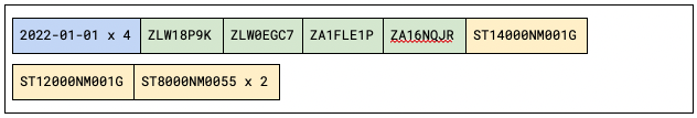
Here’s a subset of the Drive Stats data represented as CSV. We’ve omitted most of the SMART attributes to make the records more manageable.

date,serial_number,model,capacity_bytes,failure,
smart_1_normalized,smart_1_raw
2022-01-01,ZLW18P9K,ST14000NM001G,14000519643136,0,73,20467240
2022-01-01,ZLW0EGC7,ST12000NM001G,12000138625024,0,84,228715872
2022-01-01,ZA1FLE1P,ST8000NM0055,8001563222016,0,82,157857120
2022-01-01,ZA16NQJR,ST8000NM0055,8001563222016,0,84,234265456
2022-01-01,1050A084F97G,TOSHIBA MG07ACA14TA,14000519643136,0,100,0

Currently, we create a CSV file for each day’s data, comprising a record for each drive that was operational at the beginning of that day. The CSV files are each named with the appropriate date in year-month-day order, for example, 2022-06-28.csv. As mentioned above, we make each quarter’s data available as a ZIP file containing the CSV files.

At the beginning of the last Drive Stats quarter, Jan 1, 2022, we were spinning over 200,000 hard drives, so each daily file contained over 200,000 lines and occupied nearly 75MB of disk space. The ZIP file containing the Drive Stats data for the first quarter of 2022 compressed 90 files totaling 6.63GB of CSV data to a single 1.06GB file made available for download here.

Big Data Analytics in the Cloud with Trino

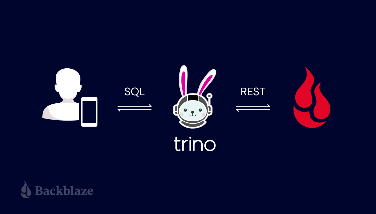
Zipped CSV files allow users to easily download, inspect, and analyze the data locally, but a new generation of tools allows us to explore and query data in situ on Backblaze B2 and other cloud storage platforms. One example is the open-source Trino query engine (formerly known as Presto SQL). Trino can natively query data in Backblaze B2, Cassandra, MySQL, and many other data sources without copying that data into its own dedicated store.

A powerful capability of Trino is that it is a distributed query engine and offers what is sometimes referred to as massively parallel processing (MPP). Thus, adding more nodes in your Trino compute cluster consistently delivers dramatically shorter query execution times. Faster results are always desirable. We achieved the results we report below running Trino on only a single node.

Note: If you are unfamiliar with Trino, the open-source project was previously known as Presto and leverages the Hadoop ecosystem.

In preparing this blog post, our team used Brian Olsen’s excellent Hive connector over MinIO file storage tutorial as a starting point for integrating Trino with Backblaze B2. The tutorial environment includes a preconfigured Docker Compose environment comprising the Trino Docker image and other required services for working with data in Backblaze B2. We brought up the environment in Docker Desktop; alternately on ThinkPads and MacBook Pros.

As a first step, we downloaded the data set for the most recent quarter, unzipped it to our local disks, and then finally reuploaded the unzipped CSV into Backblaze B2 buckets. As mentioned above, the uncompressed CSV data occupies 6.63GB of storage, so we confined our initial explorations to just a single day’s data: over 200,000 records, occupying 72.8MB.

A Word About Apache Hive

Trino accesses analytical data in Backblaze B2 and other cloud storage platforms via its Hive connector. Quoting from the Trino documentation:

The Hive connector allows querying data stored in an Apache Hive data warehouse. Hive is a combination of three components:

  • Data files in varying formats, that are typically stored in the Hadoop Distributed File System (HDFS) or in object storage systems such as Amazon S3.
  • Metadata about how the data files are mapped to schemas and tables. This metadata is stored in a database, such as MySQL, and is accessed via the Hive metastore service.
  • A query language called HiveQL. This query language is executed on a distributed computing framework such as MapReduce or Tez.

Trino only uses the first two components: the data and the metadata. It does not use HiveQL or any part of Hive’s execution environment.

The Hive connector tutorial includes Docker images for the Hive metastore service (HMS) and MariaDB, so it’s a convenient way to explore this functionality with Backblaze B2.

Configuring Trino for Backblaze B2

The tutorial uses MinIO, an open-source implementation of the Amazon S3 API, so it was straightforward to adapt the sample MinIO configuration to Backblaze B2’s S3 Compatible API by just replacing the endpoint and credentials. Here’s the b2.properties file we created:

connector.name=hive
hive.metastore.uri=thrift://hive-metastore:9083
hive.s3.path-style-access=true
hive.s3.endpoint=https://s3.us-west-004.backblazeb2.com
hive.s3.aws-access-key=
hive.s3.aws-secret-key=
hive.non-managed-table-writes-enabled=true
hive.s3select-pushdown.enabled=false
hive.storage-format=CSV
hive.allow-drop-table=true

Similarly, we edited the Hive configuration files, again replacing the MinIO configuration with the corresponding Backblaze B2 values. Here’s a sample core-site.xml:

<?xml version="1.0"?>
<configuration>

    <property>
        <name>fs.defaultFS</name>
        <value>s3a://b2-trino-getting-started</value>
    </property>


    <!-- B2 properties -->
    <property>
        <name>fs.s3a.connection.ssl.enabled</name>
        <value>true</value>
    </property>

    <property>
        <name>fs.s3a.endpoint</name>
        <value>https://s3.us-west-004.backblazeb2.com</value>
    </property>

    <property>
        <name>fs.s3a.access.key</name>
        <value><my b2 application key id></value>
    </property>

    <property>
        <name>fs.s3a.secret.key</name>
        <value><my b2 application key id></value>
    </property>

    <property>
        <name>fs.s3a.path.style.access</name>
        <value>true</value>
    </property>

    <property>
        <name>fs.s3a.impl</name>
        <value>org.apache.hadoop.fs.s3a.S3AFileSystem</value>
    </property>

</configuration>

We made a similar set of edits to metastore-site.xml and restarted the Docker instances so our changes took effect.

Uncompressed CSV

Our first test validated creating a table and running a query on a single-day CSV data set. Hive tables are configured with the directory containing the actual data files, so we uploaded 2020-01-01.csv from a local disk to data_20220101_csv/2020-01-01.csv in a Backblaze B2 bucket, opened the Trino CLI, and created a schema and a table:

CREATE SCHEMA b2.ds
WITH (location = 's3a://b2-trino-getting-started/');

USE b2.ds;

CREATE TABLE jan1_csv (
    date VARCHAR,
    serial_number VARCHAR,
    model VARCHAR,
    capacity_bytes VARCHAR,
    failure VARCHAR,
    smart_1_normalized VARCHAR,
    smart_1_raw VARCHAR,
    ...
    smart_255_normalized VARCHAR,
    smart_255_raw VARCHAR)
WITH (format = 'CSV',
    skip_header_line_count = 1,
    external_location = '
s3a://b2-trino-getting-started/data_20220101_csv');

Unfortunately, the Trino Hive connector only supports the VARCHAR data type when accessing CSV data, but, as we’ll see in a moment, we can use the CAST function in queries to convert character data to numeric and other types.

Now to run some queries! A good test is to check if all the data is there:

trino:ds> SELECT COUNT(*) FROM jan1_csv;
 _col0  
--------
 206954 
(1 row)

Query 20220629_162533_00024_qy4c6, FINISHED, 1 node
Splits: 8 total, 8 done (100.00%)
8.23 [207K rows, 69.4MB] [25.1K rows/s, 8.43MB/s]
Note: If you’re wondering about the discrepancy between the size of the CSV file–72.8MB–and the amount of data read by Trino–69.4MB–it’s accounted for in the different usage of the ‘MB’ abbreviation. For instance Mac interprets MB as a megabyte, 1,000,000 bytes, while Trino is reporting mebibytes, 1,048,576 bytes. Strictly speaking, Trino should use the abbreviation MiB. Pat opened an issue for this (with a goal of fixing it and submitting a pull request to the Trino project).

Now let’s see how many drives failed that day, grouped by the drive model:

trino:ds> SELECT model, COUNT(*) as failures 
       -> FROM jan1_csv 
       -> WHERE failure = 1 
       -> GROUP BY model 
       -> ORDER BY failures DESC;
       model        | failures 
--------------------+----------
 TOSHIBA MQ01ABF050 |        1 
 ST4000DM005        |        1 
 ST8000NM0055       |        1 
(3 rows)

Query 20220629_162609_00025_qy4c6, FINISHED, 1 node
Splits: 17 total, 17 done (100.00%)
8.23 [207K rows, 69.4MB] [25.1K rows/s, 8.43MB/s]

Notice that the query execution time is identical between the two queries. This makes sense–the time taken to run the query is dominated by the time required to download the data from Backblaze B2.

Finally, we can use the CAST function with SUM and ROUND to see how many exabytes of storage we were spinning on that day:

trino:ds> SELECT ROUND(SUM(CAST(capacity_bytes AS bigint))/1e+18, 2) FROM jan1_csv;
 _col0 
-------
  2.25 
(1 row)

Query 20220629_172703_00047_qy4c6, FINISHED, 1 node
Splits: 12 total, 12 done (100.00%)
7.83 [207K rows, 69.4MB] [26.4K rows/s, 8.86MB/s]

Although this performance may seem too long running, please note that this is against raw data. What we are highlighting here with Drive Stats data can also be used for querying data in log files. As new records are written on this append-only dataset they immediately appear as new rows in the query. This is very powerful for both real-time and near real-time analysis, and faster performance is easily achieved by scaling out the Trino cluster. Remember, Trino is a distributed query engine. For this demonstration, we have limited Trino to running on just a single node.

Compressed CSV

This is pretty neat, but not exactly fast. Extrapolating, we might expect it to take about 12 minutes to run a query against a whole quarter of Drive Stats data.

Can we improve performance? Absolutely–we simply need to reduce the amount of data that needs to be downloaded for each query!

Commonplace in the world of data analytics are data pipelines, often known as ETL for Extract, Transform, and Load. Where data is repeatedly queried, it is often advantageous to “transform” data from the raw form that it originates in into some format more optimized for the repeated queries that follow through the next stages of that data’s life cycle.

For our next test we will perform an elementary transformation of the data using a lossless compression of the CSV data with Hive’s preferred gzip format, resulting in an 11.7 MB file, 2020-01-01.csv.gz. After uploading the compressed file to data_20220101_csv_gz/2020-01-01.csv.gz, we created a second table, copying the schema from the first:

CREATE TABLE jan1_csv_gz (
	LIKE jan1_csv
)
WITH (FORMAT = 'CSV',
    EXTERNAL_LOCATION = 's3a://b2-trino-getting-started/data_20220101_csv_gz');

Trying the failure count query:

trino:ds> SELECT model, COUNT(*) as failures 
       -> FROM jan1_csv_gz 
       -> WHERE failure = 1 
       -> GROUP BY model 
       -> ORDER BY failures DESC;
       model        | failures 
--------------------+----------
 TOSHIBA MQ01ABF050 |        1 
 ST8000NM0055       |        1 
 ST4000DM005        |        1 
(3 rows)

Query 20220629_162713_00027_qy4c6, FINISHED, 1 node
Splits: 15 total, 15 done (100.00%)
2.71 [207K rows, 11.1MB] [76.4K rows/s, 4.1MB/s]

As you might expect, given that Trino has to download less than ⅙ as much data as previously, the query time fell dramatically–from just over 8 seconds to under 3 seconds. Can we do even better than this?

Enter Apache Parquet

The issue with running this kind of analytical query is that it often results in a “full table scan”–Trino has to read the model and failure fields from every record to execute the query. The row-oriented layout of CSV data means that Trino ends up reading the entire file. We can get around this by using a file format designed specifically for analytical workloads.

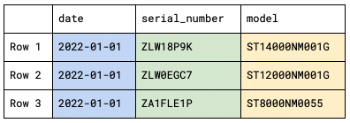
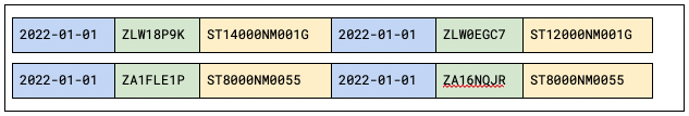
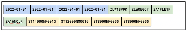
While CSV files comprise a line of text for each record, Parquet is a column-oriented, binary file format, storing the binary values for each column contiguously. Here’s a simple visualization of the difference between row and column orientation:

Table representation:

Row orientation:

Column Orientation:


Parquet also implements run-length encoding and other compression techniques. Where a series of records have the same value for a given field the Parquet file need only store the value and the number of repetitions:

The result is a compact file format well suited for analytical queries.

There are many tools to manipulate tabular data from one format to another. In this case, we wrote a very simple Python script that used the pyarrow library to do the job:

import pyarrow.csv as csv
import pyarrow.parquet as parquet

filename = '2022-01-01.csv'

parquet.write_table(csv.read_csv(filename), 
filename.replace('.csv', '.parquet'))

The resulting Parquet file occupies 12.8MB–only 1.1MB more than the gzip file. Again, we uploaded the resulting file and created a table in Trino.

CREATE TABLE jan1_parquet (
    date DATE,
    serial_number VARCHAR,
    model VARCHAR,
    capacity_bytes BIGINT,
    failure TINYINT,
    smart_1_normalized BIGINT,
    smart_1_raw BIGINT,
    ...
    smart_255_normalized BIGINT,
    smart_255_raw BIGINT)
WITH (FORMAT = 'PARQUET',
    EXTERNAL_LOCATION = 
's3a://b2-trino-getting-started/data_20220101_parquet);

Note that the conversion to Parquet automatically formatted the data using appropriate types, which we used in the table definition.

Let’s run a query and see how Parquet fares against compressed CSV:

trino:ds> SELECT model, COUNT(*) as failures 
       -> FROM jan1_parquet 
       -> WHERE failure = 1 
       -> GROUP BY model 
       -> ORDER BY failures DESC;
       model        | failures 
--------------------+----------
 TOSHIBA MQ01ABF050 |        1 
 ST4000DM005        |        1 
 ST8000NM0055       |        1 
(3 rows)

Query 20220629_163018_00031_qy4c6, FINISHED, 1 node
Splits: 15 total, 15 done (100.00%)
0.78 [207K rows, 334KB] [265K rows/s, 427KB/s]

The test query is executed in well under a second! Looking at the last line of output, we can see that the same number of rows were read, but only 334KB of data was retrieved. Trino was able to retrieve just the two columns it needed, out of the 179 columns in the file, to run the query.

Similar analytical queries execute just as efficiently. Calculating the total amount of storage in exabytes:

trino:ds> SELECT ROUND(SUM(capacity_bytes)/1e+18, 2) FROM jan1_parquet;
 _col0 
-------
  2.25 
(1 row)

Query 20220629_163058_00033_qy4c6, FINISHED, 1 node
Splits: 10 total, 10 done (100.00%)
0.83 [207K rows, 156KB] [251K rows/s, 189KB/s]

What was the capacity of the largest drive in terabytes?

trino:ds> SELECT max(capacity_bytes)/1e+12 FROM jan1_parquet;
      _col0      
-----------------
 18.000207937536 
(1 row)

Query 20220629_163139_00034_qy4c6, FINISHED, 1 node
Splits: 10 total, 10 done (100.00%)
0.80 [207K rows, 156KB] [259K rows/s, 195KB/s]

Parquet’s columnar layout excels with analytical workloads, but if we try a query more suited to an operational database, Trino has to read the entire file, as we would expect:

trino:ds> SELECT * FROM jan1_parquet WHERE serial_number = 'ZLW18P9K';
    date    | serial_number |     model     | capacity_bytes | failure
------------+---------------+---------------+----------------+--------
 2022-01-01 | ZLW18P9K      | ST14000NM001G | 14000519643136 |       0
(1 row)

Query 20220629_163206_00035_qy4c6, FINISHED, 1 node
Splits: 5 total, 5 done (100.00%)
2.05 [207K rows, 12.2MB] [101K rows/s, 5.95MB/s]

Scaling Up

After validating our Trino configuration with just a single day’s data, our next step up was to create a Parquet file containing an entire quarter. The file weighed in at 1.0GB, a little smaller than the zipped CSV.

Here’s the failed drives query for the entire quarter, limited to the top 10 results:

trino:ds> SELECT model, COUNT(*) as failures 
       -> FROM q1_2022_parquet 
       -> WHERE failure = 1 
       -> GROUP BY model 
       -> ORDER BY failures DESC 
       -> LIMIT 10;
        model         | failures 
----------------------+----------
 ST4000DM000          |      117 
 TOSHIBA MG07ACA14TA  |       88 
 ST8000NM0055         |       86 
 ST12000NM0008        |       73 
 ST8000DM002          |       38 
 ST16000NM001G        |       24 
 ST14000NM001G        |       24 
 HGST HMS5C4040ALE640 |       21 
 HGST HUH721212ALE604 |       21 
 ST12000NM001G        |       20 
(10 rows)

Query 20220629_183338_00050_qy4c6, FINISHED, 1 node
Splits: 43 total, 43 done (100.00%)
3.38 [18.8M rows, 15.8MB] [5.58M rows/s, 4.68MB/s]

Of course, those are absolute failure numbers; they don’t take account of how many of each drive model are in use. We can construct a more complex query that tells us the percentages of failed drives, by model:

trino:ds> SELECT drives.model AS model, drives.drives AS drives, 
       ->   failures.failures AS failures, 
       ->   ROUND((CAST(failures AS double)/drives)*100, 6) AS percentage
       -> FROM
       -> (
       ->   SELECT model, COUNT(*) as drives 
       ->   FROM q1_2022_parquet 
       ->   GROUP BY model
       -> ) AS drives
       -> RIGHT JOIN
       -> (
       ->   SELECT model, COUNT(*) as failures 
       ->   FROM q1_2022_parquet 
       ->   WHERE failure = 1 
       ->   GROUP BY model
       -> ) AS failures
       -> ON drives.model = failures.model
       -> ORDER BY percentage DESC
       -> LIMIT 10;
        model         | drives | failures | percentage 
----------------------+--------+----------+------------
 ST12000NM0117        |    873 |        1 |   0.114548 
 ST10000NM001G        |   1028 |        1 |   0.097276 
 HGST HUH728080ALE604 |   4504 |        3 |   0.066607 
 TOSHIBA MQ01ABF050M  |  26231 |       13 |    0.04956 
 TOSHIBA MQ01ABF050   |  24765 |       12 |   0.048455 
 ST4000DM005          |   3331 |        1 |   0.030021 
 WDC WDS250G2B0A      |   3338 |        1 |   0.029958 
 ST500LM012 HN        |  37447 |       11 |   0.029375 
 ST12000NM0007        | 118349 |       19 |   0.016054 
 ST14000NM0138        | 144333 |       17 |   0.011778 
(10 rows)

Query 20220629_191755_00010_tfuuz, FINISHED, 1 node
Splits: 82 total, 82 done (100.00%)
8.70 [37.7M rows, 31.6MB] [4.33M rows/s, 3.63MB/s]

This query took twice as long as the last one! Again, data transfer time is the limiting factor–Trino downloads the data for each subquery. A real-world deployment would take advantage of the Hive Connector’s storage caching feature to avoid repeatedly retrieving the same data.

Picking the Right Tool for the Job

You might be wondering how a relational database would stack up against the Trino/Parquet/Backblaze B2 combination. As a quick test, we installed PostgreSQL 14 on a MacBook Pro, loaded the same quarter’s data into a table, and ran the same set of queries:

Count Rows

sql_stmt=# \timing
Timing is on.
sql_stmt=# SELECT COUNT(*) FROM q1_2022;

  count   
----------
 18845260
(1 row)

Time: 1579.532 ms (00:01.580)

Absolute Number of Failures

sql_stmt=# SELECT model, COUNT(*) as failures                                                                                                          FROM q1_2022                                                                                                                                             WHERE failure = 't'                                                                                                                                      GROUP BY model                                                                                                                                           ORDER BY failures DESC                                                                                                                                   LIMIT 10;

        model         | failures 
----------------------+----------
 ST4000DM000          |      117
 TOSHIBA MG07ACA14TA  |       88
 ST8000NM0055         |       86
 ST12000NM0008        |       73
 ST8000DM002          |       38
 ST14000NM001G        |       24
 ST16000NM001G        |       24
 HGST HMS5C4040ALE640 |       21
 HGST HUH721212ALE604 |       21
 ST12000NM001G        |       20
(10 rows)

Time: 2052.019 ms (00:02.052)

Relative Number of Failures

sql_stmt=# SELECT drives.model AS model, drives.drives AS drives,                                                                                      failures.failures,                                                                                                                                       ROUND((CAST(failures AS numeric)/drives)*100, 6) AS percentage                                                                                           FROM                                                                                                                                                     (                                                                                                                                                        SELECT model, COUNT(*) as drives                                                                                                                         FROM q1_2022                                                                                                                                             GROUP BY model                                                                                                                                           ) AS drives                                                                                                                                              RIGHT JOIN                                                                                                                                               (                                                                                                                                                        SELECT model, COUNT(*) as failures                                                                                                                       FROM q1_2022                                                                                                                                             WHERE failure = 't'                                                                                                                                      GROUP BY model                                                                                                                                           ) AS failures                                                                                                                                            ON drives.model = failures.model                                                                                                                         ORDER BY percentage DESC                                                                                                                                 LIMIT 10;
        model         | drives | failures | percentage 
----------------------+--------+----------+------------
 ST12000NM0117        |    873 |        1 |   0.114548
 ST10000NM001G        |   1028 |        1 |   0.097276
 HGST HUH728080ALE604 |   4504 |        3 |   0.066607
 TOSHIBA MQ01ABF050M  |  26231 |       13 |   0.049560
 TOSHIBA MQ01ABF050   |  24765 |       12 |   0.048455
 ST4000DM005          |   3331 |        1 |   0.030021
 WDC WDS250G2B0A      |   3338 |        1 |   0.029958
 ST500LM012 HN        |  37447 |       11 |   0.029375
 ST12000NM0007        | 118349 |       19 |   0.016054
 ST14000NM0138        | 144333 |       17 |   0.011778
(10 rows)

Time: 3831.924 ms (00:03.832)

Retrieve a Single Record by Serial Number and Date

Modifying the query, since we have an entire quarter’s data:

sql_stmt=# SELECT * FROM q1_2022 WHERE serial_number = 'ZLW18P9K' AND date = '2022-01-01';
    date    | serial_number |     model     | capacity_bytes | failure
------------+---------------+---------------+----------------+-------- 
 2022-01-01 | ZLW18P9K      | ST14000NM001G | 14000519643136 | f       (1 row)

Time: 1690.091 ms (00:01.690)

For comparison, we tried to run the same query against the quarter’s data in Parquet format, but Trino crashed with an out of memory error after 58 seconds. Clearly some tuning of the default configuration is required!

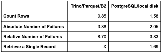
Bringing the numbers together for the quarterly data sets. All times are in seconds.

PostgreSQL is faster for most operations, but not by much, especially considering that its data is on the local SSD, rather than Backblaze B2!

It’s worth mentioning that there are yet more tuning optimizations that we have not demonstrated in this exercise. For instance, the Trino Hive connector supports storage caching. Implementing a cache yields further performance gains by avoiding repeatedly retrieving the same data from Backblaze B2. Further, Trino is a distributed query engine. Trino’s architecture is horizontally scalable. This means that Trino can also deliver shorter query run times by adding more nodes in your Trino compute cluster. We have limited all timings in this demonstration to Trino running on just a single node.

Partitioning Your Data Lake

Our final exercise was to create a single Drive Stats dataset containing all nine years of Drive Stats data. As stated above, at the time of writing the full Drive Stats dataset comprises nearly 300 million records, occupying over 90GB of disk space when in raw CSV format, rising by over 200,000 records per day, or about 75MB of CSV data.

As the dataset grows in size, an additional data engineering best practice is to include partitions.

In the introduction we mentioned that databases use optimized internal storage structures. Foremost among these are indexes. Data lakes have limited support for indexes. Data lakes do, however, support partitions. Data lake partitions are functionally similar to what databases alternately refer to as either a primary key index or index-organized tables. Regardless of the name, they effectively achieve faster data retrieval by having the data itself physically sorted. Since Drive Stats is append-only, when sorting on a date field, new records are appended to the dataset.

Having the data physically sorted greatly aids retrieval in cases that are known as range queries. To achieve fastest retrieval on a given query, it is important to only retrieve data that resolves true on the predicate in the WHERE clause. In the case of Drive Stats, for a query on only a single month or several consecutive months we get the fastest time to the result if we can read only the data for these months. Without partitioning Trino would need to do a full table scan, resulting in slower response due to the overhead of reading records for which the WHERE clause logic resolves to false. Organizing the Drive Stats data into partitions enables Trino to efficiently skip records that resolve the WHERE clause to false. Thus with partitions, many queries are far more efficient and incur the read cost only of those records whose WHERE clause logic resolves to true.

Our final transformation required a tweak to the Python script to iterate over all of the Drive Stats CSV files, writing Parquet files partitioned by year and month, so the files have prefixes of the form.

/drivestats/year={year}/month={month}/

For example:

/drivestats/year=2021/month=12/

The number of SMART attributes reported can change from one day to the next, and a single Parquet file can have only one schema, so there are one or more files with each prefix, named

{year}-{month}-{index}.parquet

For example:

2021-12-1.parquet

Again, we uploaded the resulting files and created a table in Trino.

CREATE TABLE drivestats (
    serial_number VARCHAR,
    model VARCHAR,
    capacity_bytes BIGINT,
    failure TINYINT,
    smart_1_normalized BIGINT,
    smart_1_raw BIGINT,
    ...
    smart_255_normalized BIGINT,
    smart_255_raw BIGINT,
    day SMALLINT,
    year SMALLINT,
    month SMALLINT
)
WITH (format = 'PARQUET',
 PARTITIONED_BY = ARRAY['year', 'month'],
      EXTERNAL_LOCATION = 's3a://b2-trino-getting-started/drivestats-parquet');

Note that the conversion to Parquet automatically formatted the data using appropriate types, which we used in the table definition.

This command tells Trino to scan for partition files.

CALL system.sync_partition_metadata('ds', 'drivestats', 'FULL');

Let’s run a query and see the performance against the full Drive Stats dataset in Parquet format, partitioned by month:

trino:ds> SELECT COUNT(*) FROM drivestats;
   _col0   
-----------
296413574 
(1 row)

Query 20220707_182743_00055_tshdf, FINISHED, 1 node
Splits: 412 total, 412 done (100.00%)
15.84 [296M rows, 5.63MB] [18.7M rows/s, 364KB/s]

It takes 16 seconds to count the total number of records, reading only 5.6MB of the 15.3GB total data.

Next, let’s run a query against just one month’s data:

trino:ds> SELECT COUNT(*) FROM drivestats WHERE year = 2022 AND month = 1;
  _col0  
---------
 6415842 
(1 row)

Query 20220707_184801_00059_tshdf, FINISHED, 1 node
Splits: 16 total, 16 done (100.00%)
0.85 [6.42M rows, 56KB] [7.54M rows/s, 65.7KB/s]

Counting the records for a given month takes less than a second, retrieving just 56KB of data–partitioning is working!

Now we have the entire Drive Stats data set loaded into Backblaze B2 in an efficient format and layout for running queries. Our next blog post will look at some of the queries we’ve run to clean up the data set and gain insight into nine years of hard drive metrics.

Conclusion

We hope that this article inspires you to try using Backblaze for your data analytics workloads if you’re not already doing so, and that it also serves as a useful primer to help you set up your own data lake using Backblaze B2 Cloud Storage. Our Drive Stats data is just one example of the type of data set that can be used for data analytics on Backblaze B2.

Hopefully, you too will find that Backblaze B2 Cloud Storage can be a useful, powerful, and very cost effective option for your data lake workloads.

If you’d like to get started working with analytical data in Backblaze B2, sign up here for 10 GB storage, free of charge, and get to work. If you’re already storing and querying analytical data in Backblaze B2, please let us know in the comments what tools you’re using and how it’s working out for you!

If you already work with Trino (or other data lake analytic engines), and would like connection credentials for our partitioned, Parquet, complete Drive Stats data set that is now hosted on Backblaze B2 Cloud Storage, please contact us at [email protected].
Future blog posts focused on Drive Stats and analytics will be using this complete Drive Stats dataset.

Similarly, please let us know if you would like to run a proof of concept hosting your own data in a Backblaze B2 data lake and would like the assistance of the Backblaze Developer Evangelism team.

And lastly, if you think this article may be of interest to your colleagues, we’d very much appreciate you sharing it with them.

The post Storing and Querying Analytical Data in Backblaze B2 appeared first on Backblaze Blog | Cloud Storage & Cloud Backup.

The collective thoughts of the interwebz