This post is by FactSet’s Cloud Infrastructure team, Gaurav Jain, Nathan Goodman, Geoff Wang, Daniel Cordes, Sunu Joseph, and AWS Solution Architects Amit Borulkar and Tarik Makota. In their own words, “FactSet creates flexible, open data and software solutions for tens of thousands of investment professionals around the world, which provides instant access to financial data and analytics that investors use to make crucial decisions. At FactSet, we are always working to improve the value that our products provide.”
At FactSet, our operational goal to use the AWS Cloud is to have high developer velocity alongside enterprise governance. Assigning AWS accounts per project enables the agility and isolation boundary needed by each of the project teams to innovate faster. As existing workloads are migrated and new workloads are developed in the cloud, we realized that we were operating close to thousands of AWS accounts. To have a consistent and repeatable experience for diverse project teams, we automated the AWS account creation process, various service control policies (SCP) and AWS Identity and Access Management (IAM) policies and roles associated with the accounts, and enforced policies for ongoing configuration across the accounts. This post covers our automation workflows to enable governance for thousands of AWS accounts.
AWS account creation workflow
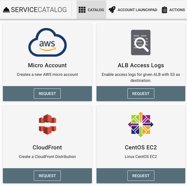
To empower our project teams to operate in the AWS Cloud in an agile manner, we developed a platform that enables AWS account creation with the default configuration customized to meet FactSet’s governance policies. These AWS accounts are provisioned with defaults such as a virtual private cloud (VPC), subnets, routing tables, IAM roles, SCP policies, add-ons for monitoring and load-balancing, and FactSet-specific governance. Developers and project team members can request a micro account for their product via this platform’s website, or do so programmatically using an API or wrap-around custom Terraform modules. The following screenshot shows a portion of the web interface that allows developers to request an AWS account.
AWS Elemental Live provides online streaming-based encoding from edge camera devices.
Through AWS Greengrass, edge devices can consume and encode video content at the edge and upload it to AWS for distribution or machine learning (ML) inference.
Currently, these services offer up to 4K encoding. Recent developments and the growing popularity of 8K content has now increased the need to distribute higher resolution content.
In this solution, you use an Amazon EC2 P3 instance to create a file-based encoding pipeline utilizing AWS Batch by first uploading a sample 8K (7680×4320) file to Amazon S3.
AWS Batch
AWS Batch enables developers, scientists, and engineers to easily and efficiently run hundreds of thousands of batch computing jobs on AWS. AWS Batch dynamically provisions the optimal quantity and type of compute resources (e.g., CPU or memory optimized instances) based on the volume and specific resource requirements of the batch jobs submitted. With AWS Batch, there is no need to install and manage batch computing software or server clusters that you use to run your jobs, allowing you to focus on analyzing results and solving problems. AWS Batch plans, schedules, and executes your batch computing workloads across the full range of AWS compute services and features, such as Amazon EC2 and Spot Instances.
P3 instances for video transcoding workloads
The P3 instance comes equipped with the NVIDIA Tesla V100 GPU. The V100 is a 16 GB 5,120 CUDA Core-GPU based on the latest Volta architecture; well suited for video coding workloads. The largest instance size in that family, p3.16xlarge, has 64 vCPU, 488 GB of RAM, 8 NVIDIA Tesla V100 GPUs, and 25 Gbps networking bandwidth.
Other than being a mainstay in computational workloads the V100 offers enhanced hardware-based encoding/decoding (NVENC/NVDEC). The following tables summarize the NVENC/NVDEC options available compared to other GPUs offered at AWS.
NVENC Support Matrix
AWS GPU instance
GPU FAMILY
GPU
H.264 (AVCHD) YUV 4:2:0
H.264 (AVCHD) YUV 4:4:4
H.264 (AVCHD) Lossless
H.265 (HEVC) 4K YUV 4:2:0
H.265 (HEVC) 4K YUV 4:4:4
H.265 (HEVC) 4K Lossless
H.265 (HEVC) 8k
G2
Kepler
GRID K520
YES
P2
Kepler (2nd Gen)
Tesla K80
YES
G3
Maxwell (2nd Gen)
Tesla M60
YES
YES
YES
YES
P3
Volta
Tesla V100
YES
YES
YES
YES
YES
YES
YES
NVDEC Support Matrix
AWS GPU instance
GPU FAMILY
GPU
MPEG-2
VC-1
H.264 (AVCHD)
H.265 (HEVC)
VP8
VP9
G2
Kepler
GRID K520
YES
YES
YES
P2
Kepler (2nd Gen)
Tesla K80
YES
YES
YES
G3
Maxwell (2nd Gen)
Tesla M60
YES
YES
YES
YES
P3
Volta
Tesla V100
YES
YES
YES
YES
YES
YES
Cinematic 8K encoding is supported using the Tesla V100 (P3 instance family) either in landscape or portrait orientations using the HEVC codec.
GPU
H264
H264_444
H264_ME
H264_WxH
HEVC
HEVC_Main10
HEVC_Lossless
HEVC_SAO
HEVC_444
HEVC_ME
HEVC_WxH
Tesla M60
+
+
+
4096x 4096
+
4096x 4096
Tesla V100
+
+
+
4096x 4096
+
+
+
+
+
+
8192x 8192
Prerequisites
To follow along with these procedures, ensure that you have the following:
An AWS account with permissions to create IAM roles and policies, as well as read and write access to S3
Registration with the NVIDIA Developer Network
Familiarity with Docker
Deployment
For deployment, you containerize the encoding pipeline. After building the underlying P3 container instance, you then use nvidia-docker2 to build the video-encoding Docker image, which is registered with Amazon Elastic Container Registry (Amazon ECR).
As shown in the following diagram, the pipeline reads an input raw YUV file from S3, then pulls the containerized encoding application to execute at scale on the P3 container instance. The encoded video file is then be transferred to S3.
The nvidia-docker2 image video encoding stack contains the following components:
NVIDIA CUDA 9.2
FFMPEG 4.0
NVIDIA Video Codec SDK 8.1
This is a relatively lengthy procedure. However, after it’s built, the underlying instance and Docker image are reusable and can be quickly deployed as part of a high performance computing (HPC) pipeline.
Creating the ECS container instance
The underlying instance can be built by selecting the Amazon Linux AMI with the p3.2xlarge instance type in a public subnet. Additionally, add an EBS volume (150 GB), which is used for the 8k input, raw yuv, and output files. Scale the storage amount for larger input files. Persist the mount in /etc/fstab. Connect to the instance over SSH and install any OS updates as well as the EPEL Release and support packages as well as the base docker-ce.
With Docker installed, pull the latest nvidia/cuda:latest image from DockerHub.
docker pull nvidia/cuda:latest
It is best at this point to run the Docker container in interactive mode. However, a Docker build file can be created afterwards. At the time of publication, only CUDA 9.0 is installed. NVIDIA has already provided the necessary repositories. Install CUDA 9.2, and support packages, inside the Docker container, referenced by the (docker) label:
First, extract the nv-codec-headers and into the directory:
(docker) make
(docker) make install
Extract the ffmpeg-4.0 directory and compile and install FFmpeg:
(docker) ./configure --enable-cuda --enable-cuvid --enable-nvenc --enable-nonfree --enable-libnpp --extra-cflags=-I/usr/local/cuda/include --extra-ldflags=-L/usr/local/cuda/lib64
(docker) make -j 4
(docker) make install
Download and extract the NVIDIA Video Codec SDK 8.1. The “Samples” directory has a preconfigured Makefile that compiles the binaries in the SDK. After it’s successful, confirm that the binaries are correctly set up.
(docker): ~/Video_Codec_SDK_8.1.24/Samples/AppEncode/AppEncCuda$ ./AppEncCuda -h
Options:
-i Input file path
-o Output file path
-s Input resolution in this form: WxH
-if Input format: iyuv nv12 yuv444 p010 yuv444p16 bgra bgra10 ayuv abgr abgr10
-gpu Ordinal of GPU to use
-codec Codec: h264 hevc
-preset Preset: default hp hq bd ll ll_hp ll_hq lossless lossless_hp
-profile H264: baseline main high high444; HEVC: main main10 frext
-444 (Only for RGB input) YUV444 encode
-rc Rate control mode: constqp vbr cbr cbr_ll_hq cbr_hq vbr_hq
-fps Frame rate
-gop Length of GOP (Group of Pictures)
-bf Number of consecutive B-frames
-bitrate Average bit rate, can be in unit of 1, K, M
-maxbitrate Max bit rate, can be in unit of 1, K, M
-vbvbufsize VBV buffer size in bits, can be in unit of 1, K, M
-vbvinit VBV initial delay in bits, can be in unit of 1, K, M
-aq Enable spatial AQ and set its stength (range 1-15, 0-auto)
-temporalaq (No value) Enable temporal AQ
-lookahead Maximum depth of lookahead (range 0-32)
-cq Target constant quality level for VBR mode (range 1-51, 0-auto)
-qmin Min QP value
-qmax Max QP value
-initqp Initial QP value
-constqp QP value for constqp rate control mode
Note: QP value can be in the form of qp_of_P_B_I or qp_P,qp_B,qp_I (no space)
Encoder Capability
# GPU H264 H264_444 H264_ME H264_WxH HEVC HEVC_Main10 HEVC_Lossless HEVC_SAO HEVC_444 HEVC_ME HEVC_WxH
0 Tesla V100-SXM2-16GB + + + 4096x4096 + + + + + + 8192x8192
Create a small script to be used for the 8K-encoding test inside the Docker container. Save the file as /root/nvenc-processor.sh. In the basic form, this script encodes using a single thread. For comparison, the same file is encoded using four threads.
(docker)
#!/bin/bash -xe
time aws s3 cp $S3_INPUT /mnt/8k.webm
time /usr/local/bin/ffmpeg -y -hwaccel cuda -i /mnt/8k.webm -c:v rawvideo -pix_fmt yuv420p /mnt/8k.yuv
time /root/Video_Codec_SDK/Samples/AppEncode/AppEncCuda/AppEncCuda -i /mnt/8k.yuv -o /mnt/8k.hevc -s 7680x4320 -codec hevc
time /root/Video_Codec_SDK/Samples/AppEncode/AppEncPerf/AppEncPerf -i /mnt/8k.yuv -s 7680x4320 -thread 4 -codec hevc
time aws s3 cp /mnt/8k.hevc $S3_OUTPUT
This script downloads a file from S3 and processes it through FFmpeg. Using the AppEncCuda and AppEncPerf methods, create the 8K-encoded file to be uploaded back to S3. Commit your Docker container into a new Docker image:
Ensure that a Docker repo has been created in Amazon ECS. Choose Repositories, Create Repository. After you open the repository, choose View Push Commands. Commit the new created image to your ECR repo.
After confirming that your image is in your ECR repo, delete all images locally in the instance:
docker rmi -f $(docker images -a -q)
Before stopping the instance, remove the ECS agent checkpoint file:
sudo rm -rf /var/lib/ecs/data/ecs_agent_data.json
Create an AMI from the instance, maintaining the attached EBS volume. Note the AMI ID.
Creating IAM role permissions
To ensure that access to ECS is controlled and to allow AWS Batch to be called, create two IAM roles:
BatchServiceRole allows AWS Batch to call services on your behalf.
ecsInstanceRole is specific to this workflow and adds permissions for S3FullAccess. This allows the container to read from and write to your S3 bucket. The following screenshot shows the example policy stack.
In AWS Batch, select the compute environment and create a managed compute environment. Assign a cluster name and min and max vCPUs values. Use the AMI ID, and IAM roles created earlier. Use the Spot pricing model with a consideration of running at 60% of the On-Demand price. Look at the current Spot price to see if more aggressive discounts are possible.
Note the cluster name. In Amazon ECS, you should see the cluster created. Next, create a job queue and associate this job queue with the compute environment created earlier. Note the job queue name.
Next, create a job definition file. This provides the job parameters to be used including mounting paths, CPU, and memory requirements.
In the AWS Batch console, create a job queue assigning a priority of 1 to the compute environment created earlier. Create a job assigning a job name, with the job definition file, and job queue. Add additional environment variables for the S3 bucket. Ensure that these buckets and input file are created.
Execute the job. In a few moments, the job should be in the Running state. Check the CloudWatch logs for an updated status of the job progression. Open the job record information and scroll down to CloudWatch metrics. The events are logged in a new AWS Batch log stream.
A 1-minute 8K YUV 4:2:0 file took approximately 10 minutes single-threaded (top panel), and 58 seconds using four threads (bottom panel). The nvenc-processor.sh script serves as a basic implementation of 8K encoding. Explore the options provided by the NVIDIA Video Codec SDK for additional encoding/decoding and transcoding options.
Conclusion
With AWS Batch, a customized container instance, and a dockerized NVIDIA video encoding platform, AWS can provide your HD, 4K, and now 8K media distribution. I invite you to incorporate this into your automated pipeline.
With some minor modification, it’s possible to trigger this pipeline after a new file is uploaded into S3. Then, execute through AWS Lambda or as part of an AWS Step Functions workflow.
One of the most common enquiries I receive at Pi Towers is “How can I get my hands on a Raspberry Pi Oracle Weather Station?” Now the answer is: “Why not build your own version using our guide?”
Tadaaaa! The BYO weather station fully assembled.
Our Oracle Weather Station
In 2016 we sent out nearly 1000 Raspberry Pi Oracle Weather Station kits to schools from around the world who had applied to be part of our weather station programme. In the original kit was a special HAT that allows the Pi to collect weather data with a set of sensors.
The original Raspberry Pi Oracle Weather Station HAT
We designed the HAT to enable students to create their own weather stations and mount them at their schools. As part of the programme, we also provide an ever-growing range of supporting resources. We’ve seen Oracle Weather Stations in great locations with a huge differences in climate, and they’ve even recorded the effects of a solar eclipse.
Our new BYO weather station guide
We only had a single batch of HATs made, and unfortunately we’ve given nearly* all the Weather Station kits away. Not only are the kits really popular, we also receive lots of questions about how to add extra sensors or how to take more precise measurements of a particular weather phenomenon. So today, to satisfy your demand for a hackable weather station, we’re launching our Build your own weather station guide!
Fun with meteorological experiments!
Our guide suggests the use of many of the sensors from the Oracle Weather Station kit, so can build a station that’s as close as possible to the original. As you know, the Raspberry Pi is incredibly versatile, and we’ve made it easy to hack the design in case you want to use different sensors.
Many other tutorials for Pi-powered weather stations don’t explain how the various sensors work or how to store your data. Ours goes into more detail. It shows you how to put together a breadboard prototype, it describes how to write Python code to take readings in different ways, and it guides you through recording these readings in a database.
There’s also a section on how to make your station weatherproof. And in case you want to move past the breadboard stage, we also help you with that. The guide shows you how to solder together all the components, similar to the original Oracle Weather Station HAT.
Who should try this build
We think this is a great project to tackle at home, at a STEM club, Scout group, or CoderDojo, and we’re sure that many of you will be chomping at the bit to get started. Before you do, please note that we’ve designed the build to be as straight-forward as possible, but it’s still fairly advanced both in terms of electronics and programming. You should read through the whole guide before purchasing any components.
The sensors and components we’re suggesting balance cost, accuracy, and easy of use. Depending on what you want to use your station for, you may wish to use different components. Similarly, the final soldered design in the guide may not be the most elegant, but we think it is achievable for someone with modest soldering experience and basic equipment.
You can build a functioning weather station without soldering with our guide, but the build will be more durable if you do solder it. If you’ve never tried soldering before, that’s OK: we have a Getting started with soldering resource plus video tutorial that will walk you through how it works step by step.
For those of you who are more experienced makers, there are plenty of different ways to put the final build together. We always like to hear about alternative builds, so please post your designs in the Weather Station forum.
Our plans for the guide
Our next step is publishing supplementary guides for adding extra functionality to your weather station. We’d love to hear which enhancements you would most like to see! Our current ideas under development include adding a webcam, making a tweeting weather station, adding a light/UV meter, and incorporating a lightning sensor. Let us know which of these is your favourite, or suggest your own amazing ideas in the comments!
*We do have a very small number of kits reserved for interesting projects or locations: a particularly cool experiment, a novel idea for how the Oracle Weather Station could be used, or places with specific weather phenomena. If have such a project in mind, please send a brief outline to [email protected], and we’ll consider how we might be able to help you.
Last year, we released Amazon Connect, a cloud-based contact center service that enables any business to deliver better customer service at low cost. This service is built based on the same technology that empowers Amazon customer service associates. Using this system, associates have millions of conversations with customers when they inquire about their shipping or order information. Because we made it available as an AWS service, you can now enable your contact center agents to make or receive calls in a matter of minutes. You can do this without having to provision any kind of hardware. 2
There are several advantages of building your contact center in the AWS Cloud, as described in our documentation. In addition, customers can extend Amazon Connect capabilities by using AWS products and the breadth of AWS services. In this blog post, we focus on how to get analytics out of the rich set of data published by Amazon Connect. We make use of an Amazon Connect data stream and create an end-to-end workflow to offer an analytical solution that can be customized based on need.
Solution overview
The following diagram illustrates the solution.
In this solution, Amazon Connect exports its contact trace records (CTRs) using Amazon Kinesis. CTRs are data streams in JSON format, and each has information about individual contacts. For example, this information might include the start and end time of a call, which agent handled the call, which queue the user chose, queue wait times, number of holds, and so on. You can enable this feature by reviewing our documentation.
In this architecture, we use Kinesis Firehose to capture Amazon Connect CTRs as raw data in an Amazon S3 bucket. We don’t use the recent feature added by Kinesis Firehose to save the data in S3 as Apache Parquet format. We use AWS Glue functionality to automatically detect the schema on the fly from an Amazon Connect data stream.
The primary reason for this approach is that it allows us to use attributes and enables an Amazon Connect administrator to dynamically add more fields as needed. Also by converting data to parquet in batch (every couple of hours) compression can be higher. However, if your requirement is to ingest the data in Parquet format on realtime, we recoment using Kinesis Firehose recently launched feature. You can review this blog post for further information.
By default, Firehose puts these records in time-series format. To make it easy for AWS Glue crawlers to capture information from new records, we use AWS Lambda to move all new records to a single S3 prefix called flatfiles. Our Lambda function is configured using S3 event notification. To comply with AWS Glue and Athena best practices, the Lambda function also converts all column names to lowercase. Finally, we also use the Lambda function to start AWS Glue crawlers. AWS Glue crawlers identify the data schema and update the AWS Glue Data Catalog, which is used by extract, transform, load (ETL) jobs in AWS Glue in the latter half of the workflow.
You can see our approach in the Lambda code following.
from __future__ import print_function
import json
import urllib
import boto3
import os
import re
s3 = boto3.resource('s3')
client = boto3.client('s3')
def convertColumntoLowwerCaps(obj):
for key in obj.keys():
new_key = re.sub(r'[\W]+', '', key.lower())
v = obj[key]
if isinstance(v, dict):
if len(v) > 0:
convertColumntoLowwerCaps(v)
if new_key != key:
obj[new_key] = obj[key]
del obj[key]
return obj
def lambda_handler(event, context):
bucket = event['Records'][0]['s3']['bucket']['name']
key = urllib.unquote_plus(event['Records'][0]['s3']['object']['key'].encode('utf8'))
try:
client.download_file(bucket, key, '/tmp/file.json')
with open('/tmp/out.json', 'w') as output, open('/tmp/file.json', 'rb') as file:
i = 0
for line in file:
for object in line.replace("}{","}\n{").split("\n"):
record = json.loads(object,object_hook=convertColumntoLowwerCaps)
if i != 0:
output.write("\n")
output.write(json.dumps(record))
i += 1
newkey = 'flatfiles/' + key.replace("/", "")
client.upload_file('/tmp/out.json', bucket,newkey)
s3.Object(bucket,key).delete()
return "success"
except Exception as e:
print(e)
print('Error coping object {} from bucket {}'.format(key, bucket))
raise e
We trigger AWS Glue crawlers based on events because this approach lets us capture any new data frame that we want to be dynamic in nature. CTR attributes are designed to offer multiple custom options based on a particular call flow. Attributes are essentially key-value pairs in nested JSON format. With the help of event-based AWS Glue crawlers, you can easily identify newer attributes automatically.
We recommend setting up an S3 lifecycle policy on the flatfiles folder that keeps records only for 24 hours. Doing this optimizes AWS Glue ETL jobs to process a subset of files rather than the entire set of records.
After we have data in the flatfiles folder, we use AWS Glue to catalog the data and transform it into Parquet format inside a folder called parquet/ctr/. The AWS Glue job performs the ETL that transforms the data from JSON to Parquet format. We use AWS Glue crawlers to capture any new data frame inside the JSON code that we want to be dynamic in nature. What this means is that when you add new attributes to an Amazon Connect instance, the solution automatically recognizes them and incorporates them in the schema of the results.
After AWS Glue stores the results in Parquet format, you can perform analytics using Amazon Redshift Spectrum, Amazon Athena, or any third-party data warehouse platform. To keep this solution simple, we have used Amazon Athena for analytics. Amazon Athena allows us to query data without having to set up and manage any servers or data warehouse platforms. Additionally, we only pay for the queries that are executed.
Try it out!
You can get started with our sample AWS CloudFormation template. This template creates the components starting from the Kinesis stream and finishes up with S3 buckets, the AWS Glue job, and crawlers. To deploy the template, open the AWS Management Console by clicking the following link.
In the console, specify the following parameters:
BucketName: The name for the bucket to store all the solution files. This name must be unique; if it’s not, template creation fails.
etlJobSchedule: The schedule in cron format indicating how often the AWS Glue job runs. The default value is every hour.
KinesisStreamName: The name of the Kinesis stream to receive data from Amazon Connect. This name must be different from any other Kinesis stream created in your AWS account.
s3interval: The interval in seconds for Kinesis Firehose to save data inside the flatfiles folder on S3. The value must between 60 and 900 seconds.
sampledata: When this parameter is set to true, sample CTR records are used. Doing this lets you try this solution without setting up an Amazon Connect instance. All examples in this walkthrough use this sample data.
Select the “I acknowledge that AWS CloudFormation might create IAM resources.” check box, and then choose Create. After the template finishes creating resources, you can see the stream name on the stack Outputs tab.
If you haven’t created your Amazon Connect instance, you can do so by following the Getting Started Guide. When you are done creating, choose your Amazon Connect instance in the console, which takes you to instance settings. Choose Data streaming to enable streaming for CTR records. Here, you can choose the Kinesis stream (defined in the KinesisStreamName parameter) that was created by the CloudFormation template.
Now it’s time to generate the data by making or receiving calls by using Amazon Connect. You can go to Amazon Connect Cloud Control Panel (CCP) to make or receive calls using a software phone or desktop phone. After a few minutes, we should see data inside the flatfiles folder. To make it easier to try this solution, we provide sample data that you can enable by setting the sampledata parameter to true in your CloudFormation template.
You can navigate to the AWS Glue console by choosing Jobs on the left navigation pane of the console. We can select our job here. In my case, the job created by CloudFormation is called glueJob-i3TULzVtP1W0; yours should be similar. You run the job by choosing Run job for Action.
After that, we wait for the AWS Glue job to run and to finish successfully. We can track the status of the job by checking the History tab.
When the job finishes running, we can check the Database section. There should be a new table created called ctr in Parquet format.
To query the data with Athena, we can select the ctr table, and for Action choose View data.
Doing this takes us to the Athena console. If you run a query, Athena shows a preview of the data.
When we can query the data using Athena, we can visualize it using Amazon QuickSight. Before connecting Amazon QuickSight to Athena, we must make sure to grant Amazon QuickSight access to Athena and the associated S3 buckets in the account. For more information on doing this, see Managing Amazon QuickSight Permissions to AWS Resources in the Amazon QuickSight User Guide. We can then create a new data set in Amazon QuickSight based on the Athena table that was created.
After setting up permissions, we can create a new analysis in Amazon QuickSight by choosing New analysis.
Then we add a new data set.
We choose Athena as the source and give the data source a name (in this case, I named it connectctr).
Choose the name of the database and the table referencing the Parquet results.
Then choose Visualize.
After that, we should see the following screen.
Now we can create some visualizations. First, search for the agent.username column, and drag it to the AutoGraph section.
We can see the agents and the number of calls for each, so we can easily see which agents have taken the largest amount of calls. If we want to see from what queues the calls came for each agent, we can add the queue.arn column to the visual.
After following all these steps, you can use Amazon QuickSight to add different columns from the call records and perform different types of visualizations. You can build dashboards that continuously monitor your connect instance. You can share those dashboards with others in your organization who might need to see this data.
Conclusion
In this post, you see how you can use services like AWS Lambda, AWS Glue, and Amazon Athena to process Amazon Connect call records. The post also demonstrates how to use AWS Lambda to preprocess files in Amazon S3 and transform them into a format that recognized by AWS Glue crawlers. Finally, the post shows how to used Amazon QuickSight to perform visualizations.
You can use the provided template to analyze your own contact center instance. Or you can take the CloudFormation template and modify it to process other data streams that can be ingested using Amazon Kinesis or stored on Amazon S3.
Luis Caro is a Big Data Consultant for AWS Professional Services. He works with our customers to provide guidance and technical assistance on big data projects, helping them improving the value of their solutions when using AWS.
Peter Dalbhanjan is a Solutions Architect for AWS based in Herndon, VA. Peter has a keen interest in evangelizing AWS solutions and has written multiple blog posts that focus on simplifying complex use cases. At AWS, Peter helps with designing and architecting variety of customer workloads.
Today, at the AWS Summit in Tokyo we announced a number of updates and new features for Amazon SageMaker. Starting today, SageMaker is available in Asia Pacific (Tokyo)! SageMaker also now supports CloudFormation. A new machine learning framework, Chainer, is now available in the SageMaker Python SDK, in addition to MXNet and Tensorflow. Finally, support for running Chainer models on several devices was added to AWS Greengrass Machine Learning.
Amazon SageMaker Chainer Estimator
Chainer is a popular, flexible, and intuitive deep learning framework. Chainer networks work on a “Define-by-Run” scheme, where the network topology is defined dynamically via forward computation. This is in contrast to many other frameworks which work on a “Define-and-Run” scheme where the topology of the network is defined separately from the data. A lot of developers enjoy the Chainer scheme since it allows them to write their networks with native python constructs and tools.
Luckily, using Chainer with SageMaker is just as easy as using a TensorFlow or MXNet estimator. In fact, it might even be a bit easier since it’s likely you can take your existing scripts and use them to train on SageMaker with very few modifications. With TensorFlow or MXNet users have to implement a train function with a particular signature. With Chainer your scripts can be a little bit more portable as you can simply read from a few environment variables like SM_MODEL_DIR, SM_NUM_GPUS, and others. We can wrap our existing script in a if __name__ == '__main__': guard and invoke it locally or on sagemaker.
import argparse
import os
if __name__ =='__main__':
parser = argparse.ArgumentParser()
# hyperparameters sent by the client are passed as command-line arguments to the script.
parser.add_argument('--epochs', type=int, default=10)
parser.add_argument('--batch-size', type=int, default=64)
parser.add_argument('--learning-rate', type=float, default=0.05)
# Data, model, and output directories
parser.add_argument('--output-data-dir', type=str, default=os.environ['SM_OUTPUT_DATA_DIR'])
parser.add_argument('--model-dir', type=str, default=os.environ['SM_MODEL_DIR'])
parser.add_argument('--train', type=str, default=os.environ['SM_CHANNEL_TRAIN'])
parser.add_argument('--test', type=str, default=os.environ['SM_CHANNEL_TEST'])
args, _ = parser.parse_known_args()
# ... load from args.train and args.test, train a model, write model to args.model_dir.
Then, we can run that script locally or use the SageMaker Python SDK to launch it on some GPU instances in SageMaker. The hyperparameters will get passed in to the script as CLI commands and the environment variables above will be autopopulated. When we call fit the input channels we pass will be populated in the SM_CHANNEL_* environment variables.
from sagemaker.chainer.estimator import Chainer
# Create my estimator
chainer_estimator = Chainer(
entry_point='example.py',
train_instance_count=1,
train_instance_type='ml.p3.2xlarge',
hyperparameters={'epochs': 10, 'batch-size': 64}
)
# Train my estimator
chainer_estimator.fit({'train': train_input, 'test': test_input})
# Deploy my estimator to a SageMaker Endpoint and get a Predictor
predictor = chainer_estimator.deploy(
instance_type="ml.m4.xlarge",
initial_instance_count=1
)
Now, instead of bringing your own docker container for training and hosting with Chainer, you can just maintain your script. You can see the full sagemaker-chainer-containers on github. One of my favorite features of the new container is built-in chainermn for easy multi-node distribution of your chainer training jobs.
There’s a lot more documentation and information available in both the README and the example notebooks.
AWS GreenGrass ML with Chainer
AWS GreenGrass ML now includes a pre-built Chainer package for all devices powered by Intel Atom, NVIDIA Jetson, TX2, and Raspberry Pi. So, now GreenGrass ML provides pre-built packages for TensorFlow, Apache MXNet, and Chainer! You can train your models on SageMaker then easily deploy it to any GreenGrass-enabled device using GreenGrass ML.
JAWS UG
I want to give a quick shout out to all of our wonderful and inspirational friends in the JAWS UG who attended the AWS Summit in Tokyo today. I’ve very much enjoyed seeing your pictures of the summit. Thanks for making Japan an amazing place for AWS developers! I can’t wait to visit again and meet with all of you.
The adoption of Apache Spark has increased significantly over the past few years, and running Spark-based application pipelines is the new normal. Spark jobs that are in an ETL (extract, transform, and load) pipeline have different requirements—you must handle dependencies in the jobs, maintain order during executions, and run multiple jobs in parallel. In most of these cases, you can use workflow scheduler tools like Apache Oozie, Apache Airflow, and even Cron to fulfill these requirements.
Apache Oozie is a widely used workflow scheduler system for Hadoop-based jobs. However, its limited UI capabilities, lack of integration with other services, and heavy XML dependency might not be suitable for some users. On the other hand, Apache Airflow comes with a lot of neat features, along with powerful UI and monitoring capabilities and integration with several AWS and third-party services. However, with Airflow, you do need to provision and manage the Airflow server. The Cron utility is a powerful job scheduler. But it doesn’t give you much visibility into the job details, and creating a workflow using Cron jobs can be challenging.
What if you have a simple use case, in which you want to run a few Spark jobs in a specific order, but you don’t want to spend time orchestrating those jobs or maintaining a separate application? You can do that today in a serverless fashion using AWS Step Functions. You can create the entire workflow in AWS Step Functions and interact with Spark on Amazon EMR through Apache Livy.
In this post, I walk you through a list of steps to orchestrate a serverless Spark-based ETL pipeline using AWS Step Functions and Apache Livy.
Input data
For the source data for this post, I use the New York City Taxi and Limousine Commission (TLC) trip record data. For a description of the data, see this detailed dictionary of the taxi data. In this example, we’ll work mainly with the following three columns for the Spark jobs.
Column name
Column description
RateCodeID
Represents the rate code in effect at the end of the trip (for example, 1 for standard rate, 2 for JFK airport, 3 for Newark airport, and so on).
FareAmount
Represents the time-and-distance fare calculated by the meter.
TripDistance
Represents the elapsed trip distance in miles reported by the taxi meter.
The trip data is in comma-separated values (CSV) format with the first row as a header. To shorten the Spark execution time, I trimmed the large input data to only 20,000 rows. During the deployment phase, the input file tripdata.csv is stored in Amazon S3 in the <<your-bucket>>/emr-step-functions/input/ folder.
The following image shows a sample of the trip data:
Solution overview
The next few sections describe how Spark jobs are created for this solution, how you can interact with Spark using Apache Livy, and how you can use AWS Step Functions to create orchestrations for these Spark applications.
At a high level, the solution includes the following steps:
Trigger the AWS Step Function state machine by passing the input file path.
The first stage in the state machine triggers an AWS Lambda
The Lambda function interacts with Apache Spark running on Amazon EMR using Apache Livy, and submits a Spark job.
The state machine waits a few seconds before checking the Spark job status.
Based on the job status, the state machine moves to the success or failure state.
Subsequent Spark jobs are submitted using the same approach.
The state machine waits a few seconds for the job to finish.
The job finishes, and the state machine updates with its final status.
Let’s take a look at the Spark application that is used for this solution.
Spark jobs
For this example, I built a Spark jar named spark-taxi.jar. It has two different Spark applications:
MilesPerRateCode – The first job that runs on the Amazon EMR cluster. This job reads the trip data from an input source and computes the total trip distance for each rate code. The output of this job consists of two columns and is stored in Apache Parquet format in the output path.
The following are the expected output columns:
rate_code – Represents the rate code for the trip.
total_distance – Represents the total trip distance for that rate code (for example, sum(trip_distance)).
RateCodeStatus – The second job that runs on the EMR cluster, but only if the first job finishes successfully. This job depends on two different input sets:
csv – The same trip data that is used for the first Spark job.
miles-per-rate – The output of the first job.
This job first reads the tripdata.csv file and aggregates the fare_amount by the rate_code. After this point, you have two different datasets, both aggregated by rate_code. Finally, the job uses the rate_code field to join two datasets and output the entire rate code status in a single CSV file.
The output columns are as follows:
rate_code_id – Represents the rate code type.
total_distance – Derived from first Spark job and represents the total trip distance.
total_fare_amount – A new field that is generated during the second Spark application, representing the total fare amount by the rate code type.
Note that in this case, you don’t need to run two different Spark jobs to generate that output. The goal of setting up the jobs in this way is just to create a dependency between the two jobs and use them within AWS Step Functions.
Both Spark applications take one input argument called rootPath. It’s the S3 location where the Spark job is stored along with input and output data. Here is a sample of the final output:
The next section discusses how you can use Apache Livy to interact with Spark applications that are running on Amazon EMR.
Using Apache Livy to interact with Apache Spark
Apache Livy provides a REST interface to interact with Spark running on an EMR cluster. Livy is included in Amazon EMR release version 5.9.0 and later. In this post, I use Livy to submit Spark jobs and retrieve job status. When Amazon EMR is launched with Livy installed, the EMR master node becomes the endpoint for Livy, and it starts listening on port 8998 by default. Livy provides APIs to interact with Spark.
Let’s look at a couple of examples how you can interact with Spark running on Amazon EMR using Livy.
To list active running jobs, you can execute the following from the EMR master node:
curl localhost:8998/sessions
If you want to do the same from a remote instance, just change localhost to the EMR hostname, as in the following (port 8998 must be open to that remote instance through the security group):
Through Spark submit, you can pass multiple arguments for the Spark job and Spark configuration settings. You can also do that using Livy, by passing the S3 path through the args parameter, as shown following:
For a detailed list of Livy APIs, see the Apache Livy REST API page. This post uses GET /batches and POST /batches.
In the next section, you create a state machine and orchestrate Spark applications using AWS Step Functions.
Using AWS Step Functions to create a Spark job workflow
AWS Step Functions automatically triggers and tracks each step and retries when it encounters errors. So your application executes in order and as expected every time. To create a Spark job workflow using AWS Step Functions, you first create a Lambda state machine using different types of states to create the entire workflow.
First, you use the Task state—a simple state in AWS Step Functions that performs a single unit of work. You also use the Wait state to delay the state machine from continuing for a specified time. Later, you use the Choice state to add branching logic to a state machine.
The following is a quick summary of how to use different states in the state machine to create the Spark ETL pipeline:
Task state – Invokes a Lambda function. The first Task state submits the Spark job on Amazon EMR, and the next Task state is used to retrieve the previous Spark job status.
Wait state – Pauses the state machine until a job completes execution.
Choice state – Each Spark job execution can return a failure, an error, or a success state So, in the state machine, you use the Choice state to create a rule that specifies the next action or step based on the success or failure of the previous step.
Here is one of my Task states, MilesPerRateCode, which simply submits a Spark job:
"MilesPerRate Job": {
"Type": "Task",
"Resource":"arn:aws:lambda:us-east-1:xxxxxx:function:blog-miles-per-rate-job-submit-function",
"ResultPath": "$.jobId",
"Next": "Wait for MilesPerRate job to complete"
}
This Task state configuration specifies the Lambda function to execute. Inside the Lambda function, it submits a Spark job through Livy using Livy’s POST API. Using ResultPath, it tells the state machine where to place the result of the executing task. As discussed in the previous section, Spark submit returns the session ID, which is captured with $.jobId and used in a later state.
The following code section shows the Lambda function, which is used to submit the MilesPerRateCode job. It uses the Python request library to submit a POST against the Livy endpoint hosted on Amazon EMR and passes the required parameters in JSON format through payload. It then parses the response, grabs id from the response, and returns it. The Next field tells the state machine which state to go to next.
Just like in the MilesPerRate job, another state submits the RateCodeStatus job, but it executes only when all previous jobs have completed successfully.
Here is the Task state in the state machine that checks the Spark job status:
Just like other states, the preceding Task executes a Lambda function, captures the result (represented by jobStatus), and passes it to the next state. The following is the Lambda function that checks the Spark job status based on a given session ID:
In the Choice state, it checks the Spark job status value, compares it with a predefined state status, and transitions the state based on the result. For example, if the status is success, move to the next state (RateCodeJobStatus job), and if it is dead, move to the MilesPerRate job failed state.
To set up this entire solution, you need to create a few AWS resources. To make it easier, I have created an AWS CloudFormation template. This template creates all the required AWS resources and configures all the resources that are needed to create a Spark-based ETL pipeline on AWS Step Functions.
This CloudFormation template requires you to pass the following four parameters during initiation.
Parameter
Description
ClusterSubnetID
The subnet where the Amazon EMR cluster is deployed and Lambda is configured to talk to this subnet.
KeyName
The name of the existing EC2 key pair to access the Amazon EMR cluster.
VPCID
The ID of the virtual private cloud (VPC) where the EMR cluster is deployed and Lambda is configured to talk to this VPC.
S3RootPath
The Amazon S3 path where all required files (input file, Spark job, and so on) are stored and the resulting data is written.
IMPORTANT: These templates are designed only to show how you can create a Spark-based ETL pipeline on AWS Step Functions using Apache Livy. They are not intended for production use without modification. And if you try this solution outside of the us-east-1 Region, download the necessary files from s3://aws-data-analytics-blog/emr-step-functions, upload the files to the buckets in your Region, edit the script as appropriate, and then run it.
To launch the CloudFormation stack, choose Launch Stack:
Launching this stack creates the following list of AWS resources.
Logical ID
Resource Type
Description
StepFunctionsStateExecutionRole
IAM role
IAM role to execute the state machine and have a trust relationship with the states service.
SparkETLStateMachine
AWS Step Functions state machine
State machine in AWS Step Functions for the Spark ETL workflow.
LambdaSecurityGroup
Amazon EC2 security group
Security group that is used for the Lambda function to call the Livy API.
RateCodeStatusJobSubmitFunction
AWS Lambda function
Lambda function to submit the RateCodeStatus job.
MilesPerRateJobSubmitFunction
AWS Lambda function
Lambda function to submit the MilesPerRate job.
SparkJobStatusFunction
AWS Lambda function
Lambda function to check the Spark job status.
LambdaStateMachineRole
IAM role
IAM role for all Lambda functions to use the lambda trust relationship.
EMRCluster
Amazon EMR cluster
EMR cluster where Livy is running and where the job is placed.
During the AWS CloudFormation deployment phase, it sets up S3 paths for input and output. Input files are stored in the <<s3-root-path>>/emr-step-functions/input/ path, whereas spark-taxi.jar is copied under <<s3-root-path>>/emr-step-functions/.
The following screenshot shows how the S3 paths are configured after deployment. In this example, I passed a bucket that I created in the AWS account s3://tm-app-demos for the S3 root path.
If the CloudFormation template completed successfully, you will see Spark-ETL-State-Machine in the AWS Step Functions dashboard, as follows:
Choose the Spark-ETL-State-Machine state machine to take a look at this implementation. The AWS CloudFormation template built the entire state machine along with its dependent Lambda functions, which are now ready to be executed.
On the dashboard, choose the newly created state machine, and then choose New execution to initiate the state machine. It asks you to pass input in JSON format. This input goes to the first state MilesPerRate Job, which eventually executes the Lambda function blog-miles-per-rate-job-submit-function.
Pass the S3 root path as input:
{
“rootPath”: “s3://tm-app-demos”
}
Then choose Start Execution:
The rootPath value is the same value that was passed when creating the CloudFormation stack. It can be an S3 bucket location or a bucket with prefixes, but it should be the same value that is used for AWS CloudFormation. This value tells the state machine where it can find the Spark jar and input file, and where it will write output files. After the state machine starts, each state/task is executed based on its definition in the state machine.
At a high level, the following represents the flow of events:
Execute the first Spark job, MilesPerRate.
The Spark job reads the input file from the location <<rootPath>>/emr-step-functions/input/tripdata.csv. If the job finishes successfully, it writes the output data to <<rootPath>>/emr-step-functions/miles-per-rate.
If the Spark job fails, it transitions to the error state MilesPerRate job failed, and the state machine stops. If the Spark job finishes successfully, it transitions to the RateCodeStatus Job state, and the second Spark job is executed.
If the second Spark job fails, it transitions to the error state RateCodeStatus job failed, and the state machine stops with the Failed status.
If this Spark job completes successfully, it writes the final output data to the <<rootPath>>/emr-step-functions/rate-code-status/ It also transitions the RateCodeStatus job finished state, and the state machine ends its execution with the Success status.
This following screenshot shows a successfully completed Spark ETL state machine:
The right side of the state machine diagram shows the details of individual states with their input and output.
When you execute the state machine for the second time, it fails because the S3 path already exists. The state machine turns red and stops at MilePerRate job failed. The following image represents that failed execution of the state machine:
You can also check your Spark application status and logs by going to the Amazon EMR console and viewing the Application history tab:
I hope this walkthrough paints a picture of how you can create a serverless solution for orchestrating Spark jobs on Amazon EMR using AWS Step Functions and Apache Livy. In the next section, I share some ideas for making this solution even more elegant.
Next steps
The goal of this post is to show a simple example that uses AWS Step Functions to create an orchestration for Spark-based jobs in a serverless fashion. To make this solution robust and production ready, you can explore the following options:
In this example, I manually initiated the state machine by passing the rootPath as input. You can instead trigger the state machine automatically. To run the ETL pipeline as soon as the files arrive in your S3 bucket, you can pass the new file path to the state machine. Because CloudWatch Events supports AWS Step Functions as a target, you can create a CloudWatch rule for an S3 event. You can then set AWS Step Functions as a target and pass the new file path to your state machine. You’re all set!
You can also improve this solution by adding an alerting mechanism in case of failures. To do this, create a Lambda function that sends an alert email and assigns that Lambda function to a Fail That way, when any part of your state fails, it triggers an email and notifies the user.
If you want to submit multiple Spark jobs in parallel, you can use the Parallel state type in AWS Step Functions. The Parallel state is used to create parallel branches of execution in your state machine.
With Lambda and AWS Step Functions, you can create a very robust serverless orchestration for your big data workload.
Cleaning up
When you’ve finished testing this solution, remember to clean up all those AWS resources that you created using AWS CloudFormation. Use the AWS CloudFormation console or AWS CLI to delete the stack named Blog-Spark-ETL-Step-Functions.
Summary
In this post, I showed you how to use AWS Step Functions to orchestrate your Spark jobs that are running on Amazon EMR. You used Apache Livy to submit jobs to Spark from a Lambda function and created a workflow for your Spark jobs, maintaining a specific order for job execution and triggering different AWS events based on your job’s outcome. Go ahead—give this solution a try, and share your experience with us!
Tanzir Musabbir is an EMR Specialist Solutions Architect with AWS. He is an early adopter of open source Big Data technologies. At AWS, he works with our customers to provide them architectural guidance for running analytics solutions on Amazon EMR, Amazon Athena & AWS Glue. Tanzir is a big Real Madrid fan and he loves to travel in his free time.
Naturebytes are making their weatherproof Wildlife Cam Case available as a standalone product for the first time, a welcome addition to the Raspberry Pi ecosystem that should take some of the hassle out of your outdoor builds.
Weatherproofing digital making projects
People often use Raspberry Pis and Camera Modules for outdoorprojects, but weatherproofing your set-up can be tricky. You need to keep water — and tiny creatures — out, but you might well need access for wires and cables, whether for power or sensors; if you’re using a camera, it’ll need something clear and cleanable in front of the lens. You can use sealant, but if you need to adjust anything that you’ve applied it to, you’ll have to remove it and redo it. While we’ve seen a few reasonable options available to buy, the choice has never been what you’d call extensive.
The Wildlife Cam Case is ideal for nature camera projects, of course, but it’ll also be useful for anyone who wants to take their Pi outdoors. It has weatherproof lenses that are transparent to visible and IR light, for all your nature observation projects. Its opening is hinged to allow easy access to your hardware, and the case has waterproof access for cables. Inside, there’s a mount for fixing any model of Raspberry Pi and camera, as well as many other components. On top of all that, the case comes with a sturdy nylon strap to make it easy to attach it to a post or a tree.
Order yours now!
At the moment, Naturebytes are producing a limited run of the cases. The first batch of 50 are due to be dispatched next week to arrive just in time for the Bank Holiday weekend in the UK, so get them while they’re hot. It’s the perfect thing for recording a timelapse of exactly how quickly the slugs obliterate your vegetable seedlings, and of lots more heartening things that must surely happen in gardens other than mine.
As you can see from my EC2 Instance History post, we add new instance types on a regular and frequent basis. Driven by increasingly powerful processors and designed to address an ever-widening set of use cases, the size and diversity of this list reflects the equally diverse group of EC2 customers!
Near the bottom of that list you will find the new compute-intensive C5 instances. With a 25% to 50% improvement in price-performance over the C4 instances, the C5 instances are designed for applications like batch and log processing, distributed and or real-time analytics, high-performance computing (HPC), ad serving, highly scalable multiplayer gaming, and video encoding. Some of these applications can benefit from access to high-speed, ultra-low latency local storage. For example, video encoding, image manipulation, and other forms of media processing often necessitates large amounts of I/O to temporary storage. While the input and output files are valuable assets and are typically stored as Amazon Simple Storage Service (S3) objects, the intermediate files are expendable. Similarly, batch and log processing runs in a race-to-idle model, flushing volatile data to disk as fast as possible in order to make full use of compute resources.
New C5d Instances with Local Storage In order to meet this need, we are introducing C5 instances equipped with local NVMe storage. Available for immediate use in 5 regions, these instances are a great fit for the applications that I described above, as well as others that you will undoubtedly dream up! Here are the specs:
Instance Name
vCPUs
RAM
Local Storage
EBS Bandwidth
Network Bandwidth
c5d.large
2
4 GiB
1 x 50 GB NVMe SSD
Up to 2.25 Gbps
Up to 10 Gbps
c5d.xlarge
4
8 GiB
1 x 100 GB NVMe SSD
Up to 2.25 Gbps
Up to 10 Gbps
c5d.2xlarge
8
16 GiB
1 x 225 GB NVMe SSD
Up to 2.25 Gbps
Up to 10 Gbps
c5d.4xlarge
16
32 GiB
1 x 450 GB NVMe SSD
2.25 Gbps
Up to 10 Gbps
c5d.9xlarge
36
72 GiB
1 x 900 GB NVMe SSD
4.5 Gbps
10 Gbps
c5d.18xlarge
72
144 GiB
2 x 900 GB NVMe SSD
9 Gbps
25 Gbps
Other than the addition of local storage, the C5 and C5d share the same specs. Both are powered by 3.0 GHz Intel Xeon Platinum 8000-series processors, optimized for EC2 and with full control over C-states on the two largest sizes, giving you the ability to run two cores at up to 3.5 GHz using Intel Turbo Boost Technology.
You can use any AMI that includes drivers for the Elastic Network Adapter (ENA) and NVMe; this includes the latest Amazon Linux, Microsoft Windows (Server 2008 R2, Server 2012, Server 2012 R2 and Server 2016), Ubuntu, RHEL, SUSE, and CentOS AMIs.
Here are a couple of things to keep in mind about the local NVMe storage:
Naming – You don’t have to specify a block device mapping in your AMI or during the instance launch; the local storage will show up as one or more devices (/dev/nvme*1 on Linux) after the guest operating system has booted.
Encryption – Each local NVMe device is hardware encrypted using the XTS-AES-256 block cipher and a unique key. Each key is destroyed when the instance is stopped or terminated.
Lifetime – Local NVMe devices have the same lifetime as the instance they are attached to, and do not stick around after the instance has been stopped or terminated.
Available Now C5d instances are available in On-Demand, Reserved Instance, and Spot form in the US East (N. Virginia), US West (Oregon), EU (Ireland), US East (Ohio), and Canada (Central) Regions. Prices vary by Region, and are just a bit higher than for the equivalent C5 instances.
As a serverless computing platform that supports Java 8 runtime, AWS Lambda makes it easy to run any type of Java function simply by uploading a JAR file. To help define not only a Lambda serverless application but also Amazon API Gateway, Amazon DynamoDB, and other related services, the AWS Serverless Application Model (SAM) allows developers to use a simple AWS CloudFormation template.
AWS provides the AWS Toolkit for Eclipse that supports both Lambda and SAM. AWS also gives customers an easy way to create Lambda functions and SAM applications in Java using the AWS Command Line Interface (AWS CLI). After you build a JAR file, all you have to do is type the following commands:
To consolidate these steps, customers can use Archetype by Apache Maven. Archetype uses a predefined package template that makes getting started to develop a function exceptionally simple.
In this post, I introduce a Maven archetype that allows you to create a skeleton of AWS SAM for a Java function. Using this archetype, you can generate a sample Java code example and an accompanying SAM template to deploy it on AWS Lambda by a single Maven action.
Prerequisites
Make sure that the following software is installed on your workstation:
Java
Maven
AWS CLI
(Optional) AWS SAM CLI
Install Archetype
After you’ve set up those packages, install Archetype with the following commands:
git clone https://github.com/awslabs/aws-serverless-java-archetype
cd aws-serverless-java-archetype
mvn install
These are one-time operations, so you don’t run them for every new package. If you’d like, you can add Archetype to your company’s Maven repository so that other developers can use it later.
With those packages installed, you’re ready to develop your new Lambda Function.
Start a project
Now that you have the archetype, customize it and run the code:
cd /path/to/project_home
mvn archetype:generate \
-DarchetypeGroupId=com.amazonaws.serverless.archetypes \
-DarchetypeArtifactId=aws-serverless-java-archetype \
-DarchetypeVersion=1.0.0 \
-DarchetypeRepository=local \ # Forcing to use local maven repository
-DinteractiveMode=false \ # For batch mode
# You can also specify properties below interactively if you omit the line for batch mode
-DgroupId=YOUR_GROUP_ID \
-DartifactId=YOUR_ARTIFACT_ID \
-Dversion=YOUR_VERSION \
-DclassName=YOUR_CLASSNAME
You should have a directory called YOUR_ARTIFACT_ID that contains the files and folders shown below:
The sample code is a working example. If you install SAM CLI, you can invoke it just by the command below:
cd YOUR_ARTIFACT_ID
mvn -P invoke verify
[INFO] Scanning for projects...
[INFO]
[INFO] ---------------------------< com.riywo:foo >----------------------------
[INFO] Building foo 1.0
[INFO] --------------------------------[ jar ]---------------------------------
...
[INFO] --- maven-jar-plugin:3.0.2:jar (default-jar) @ foo ---
[INFO] Building jar: /private/tmp/foo/target/foo-1.0.jar
[INFO]
[INFO] --- maven-shade-plugin:3.1.0:shade (shade) @ foo ---
[INFO] Including com.amazonaws:aws-lambda-java-core:jar:1.2.0 in the shaded jar.
[INFO] Replacing /private/tmp/foo/target/lambda.jar with /private/tmp/foo/target/foo-1.0-shaded.jar
[INFO]
[INFO] --- exec-maven-plugin:1.6.0:exec (sam-local-invoke) @ foo ---
2018/04/06 16:34:35 Successfully parsed template.yaml
2018/04/06 16:34:35 Connected to Docker 1.37
2018/04/06 16:34:35 Fetching lambci/lambda:java8 image for java8 runtime...
java8: Pulling from lambci/lambda
Digest: sha256:14df0a5914d000e15753d739612a506ddb8fa89eaa28dcceff5497d9df2cf7aa
Status: Image is up to date for lambci/lambda:java8
2018/04/06 16:34:37 Invoking Package.Example::handleRequest (java8)
2018/04/06 16:34:37 Decompressing /tmp/foo/target/lambda.jar
2018/04/06 16:34:37 Mounting /private/var/folders/x5/ldp7c38545v9x5dg_zmkr5kxmpdprx/T/aws-sam-local-1523000077594231063 as /var/task:ro inside runtime container
START RequestId: a6ae19fe-b1b0-41e2-80bc-68a40d094d74 Version: $LATEST
Log output: Greeting is 'Hello Tim Wagner.'
END RequestId: a6ae19fe-b1b0-41e2-80bc-68a40d094d74
REPORT RequestId: a6ae19fe-b1b0-41e2-80bc-68a40d094d74 Duration: 96.60 ms Billed Duration: 100 ms Memory Size: 128 MB Max Memory Used: 7 MB
{"greetings":"Hello Tim Wagner."}
[INFO] ------------------------------------------------------------------------
[INFO] BUILD SUCCESS
[INFO] ------------------------------------------------------------------------
[INFO] Total time: 10.452 s
[INFO] Finished at: 2018-04-06T16:34:40+09:00
[INFO] ------------------------------------------------------------------------
This maven goal invokes sam local invoke -e event.json, so you can see the sample output to greet Tim Wagner.
To deploy this application to AWS, you need an Amazon S3 bucket to upload your package. You can use the following command to create a bucket if you want:
aws s3 mb s3://YOUR_BUCKET --region YOUR_REGION
Now, you can deploy your application by just one command!
mvn deploy \
-DawsRegion=YOUR_REGION \
-Ds3Bucket=YOUR_BUCKET \
-DstackName=YOUR_STACK
[INFO] Scanning for projects...
[INFO]
[INFO] ---------------------------< com.riywo:foo >----------------------------
[INFO] Building foo 1.0
[INFO] --------------------------------[ jar ]---------------------------------
...
[INFO] --- exec-maven-plugin:1.6.0:exec (sam-package) @ foo ---
Uploading to aws-serverless-java/com.riywo:foo:1.0/924732f1f8e4705c87e26ef77b080b47 11657 / 11657.0 (100.00%)
Successfully packaged artifacts and wrote output template to file target/sam.yaml.
Execute the following command to deploy the packaged template
aws cloudformation deploy --template-file /private/tmp/foo/target/sam.yaml --stack-name <YOUR STACK NAME>
[INFO]
[INFO] --- maven-deploy-plugin:2.8.2:deploy (default-deploy) @ foo ---
[INFO] Skipping artifact deployment
[INFO]
[INFO] --- exec-maven-plugin:1.6.0:exec (sam-deploy) @ foo ---
Waiting for changeset to be created..
Waiting for stack create/update to complete
Successfully created/updated stack - archetype
[INFO] ------------------------------------------------------------------------
[INFO] BUILD SUCCESS
[INFO] ------------------------------------------------------------------------
[INFO] Total time: 37.176 s
[INFO] Finished at: 2018-04-06T16:41:02+09:00
[INFO] ------------------------------------------------------------------------
Maven automatically creates a shaded JAR file, uploads it to your S3 bucket, replaces template.yaml, and creates and updates the CloudFormation stack.
To customize the process, modify the pom.xml file. For example, to avoid typing values for awsRegion, s3Bucket or stackName, write them inside pom.xml and check in your VCS. Afterward, you and the rest of your team can deploy the function by typing just the following command:
mvn deploy
Options
Lambda Java 8 runtime has some types of handlers: POJO, Simple type and Stream. The default option of this archetype is POJO style, which requires to create request and response classes, but they are baked by the archetype by default. If you want to use other type of handlers, you can use handlerType property like below:
## POJO type (default)
mvn archetype:generate \
...
-DhandlerType=pojo
## Simple type - String
mvn archetype:generate \
...
-DhandlerType=simple
### Stream type
mvn archetype:generate \
...
-DhandlerType=stream
Also, Lambda Java 8 runtime supports two types of Logging class: Log4j 2 and LambdaLogger. This archetype creates LambdaLogger implementation by default, but you can use Log4j 2 if you want:
If you use LambdaLogger, you can delete ./src/main/resources/log4j2.xml. See documentation for more details.
Conclusion
So, what’s next? Develop your Lambda function locally and type the following command: mvn deploy !
With this Archetype code example, available on GitHub repo, you should be able to deploy Lambda functions for Java 8 in a snap. If you have any questions or comments, please submit them below or leave them on GitHub.
Contributed by Shea Lutton, AWS Cloud Infrastructure Architect
Amazon Simple Queue Service (Amazon SQS) is a fully managed queuing service that helps decouple applications, distributed systems, and microservices to increase fault tolerance. SQS queues come in two distinct types:
Standard SQS queues are able to scale to enormous throughput with at-least-once delivery.
FIFO queues are designed to guarantee that messages are processed exactly once in the exact order that they are received and have a default rate of 300 transactions per second.
As customers explore SQS FIFO queues, they often have questions about how the behavior works when messages arrive and are consumed. This post walks through some common situations to identify the exact behavior that you can expect. It also covers the behavior of message groups in depth and explains why message groups are key to understanding how FIFO queues work.
The simple case
Suppose that you run a major auction platform where people buy and sell a wide range of products. Your platform requires that transactions from buyers and sellers get processed in exactly the order received. Here’s how a FIFO queue helps you keep all your transactions in one straight flow.
A seller currently is holding an auction for a laptop, and three different bids are received for the same price. Ties are awarded to the first bidder at that price so it is important to track which arrived first. Your auction platform receives the three bids and sends them to a FIFO queue before they are processed.
Now observe how messages leave the queue. When your consumer asks for a batch of up to 10 messages, SQS starts filling the batch with the oldest message (bid A1). It keeps filling until either the batch is full or the queue is empty. In this case, the batch contains the three messages and the queue is now empty. After a batch has left the queue, SQS considers that batch of messages to be “in-flight” until the consumer either deletes them or the batch’s visibility timer expires.
When you have a single consumer, this is easy to envision. The consumer gets a batch of messages (now in-flight), does its processing, and deletes the messages. That consumer is then ready to ask for the next batch of messages.
The critical thing to keep in mind is that SQS won’t release the next batch of messages until the first batch has been deleted. By adding more messages to the queue, you can see more interesting behaviors. Imagine that a burst of 11 bids is sent to your FIFO queue, with two bids for Auction A arriving last.
The FIFO queue now has at least two batches of messages in it. When your single consumer requests the first batch of 10 messages, it receives a batch starting with B1 and ending with A1. Later, after the first batch has been deleted, the consumer can get the second batch of messages containing the final A2 message from the queue.
Adding complexity with multiple message groups
A new challenge arises. Your auction platform is getting busier and your dev team added a number of new features. The combination of increased messages and extra processing time for the new features means that a single consumer is too slow. The solution is to scale to have more consumers and process messages in parallel.
To work in parallel, your team realized that only the messages related to a single auction must be kept in order. All transactions for Auction A need to be kept in order and so do all transactions for Auction B. But the two auctions are independent and it does not matter which auctions transactions are processed first.
FIFO can handle that case with a feature called message groups. Each transaction related to Auction A is placed by your producer into message group A, and so on. In the diagram below, Auction A and Auction B each received three bid transactions, with bid B1 arriving first. The FIFO queue always keeps transactions within a message group in the order in which they arrived.
How is this any different than earlier examples? The consumer now gets the messages ordered by message groups, all the B group messages followed by all the A group messages. Multiple message groups create the possibility of using multiple consumers, which I explain in a moment. If FIFO can’t fill up a batch of messages with a single message group, FIFO can place more than one message group in a batch of messages. But whenever possible, the queue gives you a full batch of messages from the same group.
The order of messages leaving a FIFO queue is governed by three rules:
Return the oldest message where no other message in the same message group is currently in-flight.
Return as many messages from the same message group as possible.
If a message batch is still not full, go back to rule 1.
To see this behavior, add a second consumer and insert many more messages into the queue. For simplicity, the delete message action has been omitted in these diagrams but it is assumed that all messages in a batch are processed successfully by the consumer and the batch is properly deleted immediately after.
In this example, there are 11 Group A and 11 Group B transactions arriving in interleaved order and a second consumer has been added. Consumer 1 asks for a group of 10 messages and receives 10 Group A messages. Consumer 2 then asks for 10 messages but SQS knows that Group A is in flight, so it releases 10 Group B messages. The two consumers are now processing two batches of messages in parallel, speeding up throughput and then deleting their batches. When Consumer 1 requests the next batch of messages, it receives the remaining two messages, one from Group A and one from Group B.
Consider this nuanced detail from the example above. What would happen if Consumer 1 was on a faster server and processed its first batch of messages before Consumer 2 could mark its messages for deletion? See if you can predict the behavior before looking at the answer.
If Consumer 2 has not deleted its Group B messages yet when Consumer 1 asks for the next batch, then the FIFO queue considers Group B to still be in flight. It does not release any more Group B messages. Consumer 1 gets only the remaining Group A message. Later, after Consumer 2 has deleted its first batch, the remaining Group B message is released.
Conclusion
I hope this post answered your questions about how Amazon SQS FIFO queues work and why message groups are helpful. If you’re interested in exploring SQS FIFO queues further, here are a few ideas to get you started:
Create an Amazon SQS FIFO queue with three simple commands in the SQS console
Amazon Kinesis Data Firehose is the easiest way to capture and stream data into a data lake built on Amazon S3. This data can be anything—from AWS service logs like AWS CloudTrail log files, Amazon VPC Flow Logs, Application Load Balancer logs, and others. It can also be IoT events, game events, and much more. To efficiently query this data, a time-consuming ETL (extract, transform, and load) process is required to massage and convert the data to an optimal file format, which increases the time to insight. This situation is less than ideal, especially for real-time data that loses its value over time.
To solve this common challenge, Kinesis Data Firehose can now save data to Amazon S3 in Apache Parquet or Apache ORC format. These are optimized columnar formats that are highly recommended for best performance and cost-savings when querying data in S3. This feature directly benefits you if you use Amazon Athena, Amazon Redshift, AWS Glue, Amazon EMR, or any other big data tools that are available from the AWS Partner Network and through the open-source community.
Amazon Connect is a simple-to-use, cloud-based contact center service that makes it easy for any business to provide a great customer experience at a lower cost than common alternatives. Its open platform design enables easy integration with other systems. One of those systems is Amazon Kinesis—in particular, Kinesis Data Streams and Kinesis Data Firehose.
What’s really exciting is that you can now save events from Amazon Connect to S3 in Apache Parquet format. You can then perform analytics using Amazon Athena and Amazon Redshift Spectrum in real time, taking advantage of this key performance and cost optimization. Of course, Amazon Connect is only one example. This new capability opens the door for a great deal of opportunity, especially as organizations continue to build their data lakes.
Amazon Connect includes an array of analytics views in the Administrator dashboard. But you might want to run other types of analysis. In this post, I describe how to set up a data stream from Amazon Connect through Kinesis Data Streams and Kinesis Data Firehose and out to S3, and then perform analytics using Athena and Amazon Redshift Spectrum. I focus primarily on the Kinesis Data Firehose support for Parquet and its integration with the AWS Glue Data Catalog, Amazon Athena, and Amazon Redshift.
Solution overview
Here is how the solution is laid out:
The following sections walk you through each of these steps to set up the pipeline.
1. Define the schema
When Kinesis Data Firehose processes incoming events and converts the data to Parquet, it needs to know which schema to apply. The reason is that many times, incoming events contain all or some of the expected fields based on which values the producers are advertising. A typical process is to normalize the schema during a batch ETL job so that you end up with a consistent schema that can easily be understood and queried. Doing this introduces latency due to the nature of the batch process. To overcome this issue, Kinesis Data Firehose requires the schema to be defined in advance.
To see the available columns and structures, see Amazon Connect Agent Event Streams. For the purpose of simplicity, I opted to make all the columns of type String rather than create the nested structures. But you can definitely do that if you want.
The simplest way to define the schema is to create a table in the Amazon Athena console. Open the Athena console, and paste the following create table statement, substituting your own S3 bucket and prefix for where your event data will be stored. A Data Catalog database is a logical container that holds the different tables that you can create. The default database name shown here should already exist. If it doesn’t, you can create it or use another database that you’ve already created.
That’s all you have to do to prepare the schema for Kinesis Data Firehose.
2. Define the data streams
Next, you need to define the Kinesis data streams that will be used to stream the Amazon Connect events. Open the Kinesis Data Streams console and create two streams. You can configure them with only one shard each because you don’t have a lot of data right now.
3. Define the Kinesis Data Firehose delivery stream for Parquet
Let’s configure the Data Firehose delivery stream using the data stream as the source and Amazon S3 as the output. Start by opening the Kinesis Data Firehose console and creating a new data delivery stream. Give it a name, and associate it with the Kinesis data stream that you created in Step 2.
As shown in the following screenshot, enable Record format conversion (1) and choose Apache Parquet (2). As you can see, Apache ORC is also supported. Scroll down and provide the AWS Glue Data Catalog database name (3) and table names (4) that you created in Step 1. Choose Next.
To make things easier, the output S3 bucket and prefix fields are automatically populated using the values that you defined in the LOCATION parameter of the create table statement from Step 1. Pretty cool. Additionally, you have the option to save the raw events into another location as defined in the Source record S3 backup section. Don’t forget to add a trailing forward slash “ / “ so that Data Firehose creates the date partitions inside that prefix.
On the next page, in the S3 buffer conditions section, there is a note about configuring a large buffer size. The Parquet file format is highly efficient in how it stores and compresses data. Increasing the buffer size allows you to pack more rows into each output file, which is preferred and gives you the most benefit from Parquet.
Compression using Snappy is automatically enabled for both Parquet and ORC. You can modify the compression algorithm by using the Kinesis Data Firehose API and update the OutputFormatConfiguration.
Be sure to also enable Amazon CloudWatch Logs so that you can debug any issues that you might run into.
Lastly, finalize the creation of the Firehose delivery stream, and continue on to the next section.
4. Set up the Amazon Connect contact center
After setting up the Kinesis pipeline, you now need to set up a simple contact center in Amazon Connect. The Getting Started page provides clear instructions on how to set up your environment, acquire a phone number, and create an agent to accept calls.
After setting up the contact center, in the Amazon Connect console, choose your Instance Alias, and then choose Data Streaming. Under Agent Event, choose the Kinesis data stream that you created in Step 2, and then choose Save.
At this point, your pipeline is complete. Agent events from Amazon Connect are generated as agents go about their day. Events are sent via Kinesis Data Streams to Kinesis Data Firehose, which converts the event data from JSON to Parquet and stores it in S3. Athena and Amazon Redshift Spectrum can simply query the data without any additional work.
So let’s generate some data. Go back into the Administrator console for your Amazon Connect contact center, and create an agent to handle incoming calls. In this example, I creatively named mine Agent One. After it is created, Agent One can get to work and log into their console and set their availability to Available so that they are ready to receive calls.
To make the data a bit more interesting, I also created a second agent, Agent Two. I then made some incoming and outgoing calls and caused some failures to occur, so I now have enough data available to analyze.
5. Analyze the data with Athena
Let’s open the Athena console and run some queries. One thing you’ll notice is that when we created the schema for the dataset, we defined some of the fields as Strings even though in the documentation they were complex structures. The reason for doing that was simply to show some of the flexibility of Athena to be able to parse JSON data. However, you can define nested structures in your table schema so that Kinesis Data Firehose applies the appropriate schema to the Parquet file.
Let’s run the first query to see which agents have logged into the system.
The query might look complex, but it’s fairly straightforward:
WITH dataset AS (
SELECT
from_iso8601_timestamp(eventtimestamp) AS event_ts,
eventtype,
-- CURRENT STATE
json_extract_scalar(
currentagentsnapshot,
'$.agentstatus.name') AS current_status,
from_iso8601_timestamp(
json_extract_scalar(
currentagentsnapshot,
'$.agentstatus.starttimestamp')) AS current_starttimestamp,
json_extract_scalar(
currentagentsnapshot,
'$.configuration.firstname') AS current_firstname,
json_extract_scalar(
currentagentsnapshot,
'$.configuration.lastname') AS current_lastname,
json_extract_scalar(
currentagentsnapshot,
'$.configuration.username') AS current_username,
json_extract_scalar(
currentagentsnapshot,
'$.configuration.routingprofile.defaultoutboundqueue.name') AS current_outboundqueue,
json_extract_scalar(
currentagentsnapshot,
'$.configuration.routingprofile.inboundqueues[0].name') as current_inboundqueue,
-- PREVIOUS STATE
json_extract_scalar(
previousagentsnapshot,
'$.agentstatus.name') as prev_status,
from_iso8601_timestamp(
json_extract_scalar(
previousagentsnapshot,
'$.agentstatus.starttimestamp')) as prev_starttimestamp,
json_extract_scalar(
previousagentsnapshot,
'$.configuration.firstname') as prev_firstname,
json_extract_scalar(
previousagentsnapshot,
'$.configuration.lastname') as prev_lastname,
json_extract_scalar(
previousagentsnapshot,
'$.configuration.username') as prev_username,
json_extract_scalar(
previousagentsnapshot,
'$.configuration.routingprofile.defaultoutboundqueue.name') as current_outboundqueue,
json_extract_scalar(
previousagentsnapshot,
'$.configuration.routingprofile.inboundqueues[0].name') as prev_inboundqueue
from kfhconnectblog
where eventtype <> 'HEART_BEAT'
)
SELECT
current_status as status,
current_username as username,
event_ts
FROM dataset
WHERE eventtype = 'LOGIN' AND current_username <> ''
ORDER BY event_ts DESC
The query output looks something like this:
Here is another query that shows the sessions each of the agents engaged with. It tells us where they were incoming or outgoing, if they were completed, and where there were missed or failed calls.
WITH src AS (
SELECT
eventid,
json_extract_scalar(currentagentsnapshot, '$.configuration.username') as username,
cast(json_extract(currentagentsnapshot, '$.contacts') AS ARRAY(JSON)) as c,
cast(json_extract(previousagentsnapshot, '$.contacts') AS ARRAY(JSON)) as p
from kfhconnectblog
),
src2 AS (
SELECT *
FROM src CROSS JOIN UNNEST (c, p) AS contacts(c_item, p_item)
),
dataset AS (
SELECT
eventid,
username,
json_extract_scalar(c_item, '$.contactid') as c_contactid,
json_extract_scalar(c_item, '$.channel') as c_channel,
json_extract_scalar(c_item, '$.initiationmethod') as c_direction,
json_extract_scalar(c_item, '$.queue.name') as c_queue,
json_extract_scalar(c_item, '$.state') as c_state,
from_iso8601_timestamp(json_extract_scalar(c_item, '$.statestarttimestamp')) as c_ts,
json_extract_scalar(p_item, '$.contactid') as p_contactid,
json_extract_scalar(p_item, '$.channel') as p_channel,
json_extract_scalar(p_item, '$.initiationmethod') as p_direction,
json_extract_scalar(p_item, '$.queue.name') as p_queue,
json_extract_scalar(p_item, '$.state') as p_state,
from_iso8601_timestamp(json_extract_scalar(p_item, '$.statestarttimestamp')) as p_ts
FROM src2
)
SELECT
username,
c_channel as channel,
c_direction as direction,
p_state as prev_state,
c_state as current_state,
c_ts as current_ts,
c_contactid as id
FROM dataset
WHERE c_contactid = p_contactid
ORDER BY id DESC, current_ts ASC
The query output looks similar to the following:
6. Analyze the data with Amazon Redshift Spectrum
With Amazon Redshift Spectrum, you can query data directly in S3 using your existing Amazon Redshift data warehouse cluster. Because the data is already in Parquet format, Redshift Spectrum gets the same great benefits that Athena does.
Here is a simple query to show querying the same data from Amazon Redshift. Note that to do this, you need to first create an external schema in Amazon Redshift that points to the AWS Glue Data Catalog.
SELECT
eventtype,
json_extract_path_text(currentagentsnapshot,'agentstatus','name') AS current_status,
json_extract_path_text(currentagentsnapshot, 'configuration','firstname') AS current_firstname,
json_extract_path_text(currentagentsnapshot, 'configuration','lastname') AS current_lastname,
json_extract_path_text(
currentagentsnapshot,
'configuration','routingprofile','defaultoutboundqueue','name') AS current_outboundqueue,
FROM default_schema.kfhconnectblog
The following shows the query output:
Summary
In this post, I showed you how to use Kinesis Data Firehose to ingest and convert data to columnar file format, enabling real-time analysis using Athena and Amazon Redshift. This great feature enables a level of optimization in both cost and performance that you need when storing and analyzing large amounts of data. This feature is equally important if you are investing in building data lakes on AWS.
Roy Hasson is a Global Business Development Manager for AWS Analytics. He works with customers around the globe to design solutions to meet their data processing, analytics and business intelligence needs. Roy is big Manchester United fan cheering his team on and hanging out with his family.
Since our last System and Organization Control (SOC) audit, our service and compliance teams have been working to increase the number of AWS Services in scope prioritized based on customer requests. Today, we’re happy to report 11 services are newly SOC compliant, which is a 21 percent increase in the last six months.
With the addition of the following 11 new services, you can now select from a total of 62 SOC-compliant services. To see the full list, go to our Services in Scope by Compliance Program page:
Our latest SOC 1, 2, and 3 reports covering the period from October 1, 2017 to March 31, 2018 are now available. The SOC 1 and 2 reports are available on-demand through AWS Artifact by logging into the AWS Management Console. The SOC 3 report can be downloaded here.
Finally, prospective customers can read our SOC 1 and 2 reports by reaching out to AWS Compliance.
Want more AWS Security news? Follow us on Twitter.
EC2 Spot Fleets are really cool. You can launch a fleet of Spot Instances that spans EC2 instance types and Availability Zones without having to write custom code to discover capacity or monitor prices. You can set the target capacity (the size of the fleet) in units that are meaningful to your application and have Spot Fleet create and then maintain the fleet on your behalf. Our customers are creating Spot Fleets of all sizes. For example, one financial service customer runs Monte Carlo simulations across 10 different EC2 instance types. They routinely make requests for hundreds of thousands of vCPUs and count on Spot Fleet to give them access to massive amounts of capacity at the best possible price.
EC2 Fleet Today we are extending and generalizing the set-it-and-forget-it model that we pioneered in Spot Fleet with EC2 Fleet, a new building block that gives you the ability to create fleets that are composed of a combination of EC2 On-Demand, Reserved, and Spot Instances with a single API call. You tell us what you need, capacity and instance-wise, and we’ll handle all the heavy lifting. We will launch, manage, monitor and scale instances as needed, without the need for scaffolding code.
You can specify the capacity of your fleet in terms of instances, vCPUs, or application-oriented units, and also indicate how much of the capacity should be fulfilled by Spot Instances. The application-oriented units allow you to specify the relative power of each EC2 instance type in a way that directly maps to the needs of your application. All three capacity specification options (instances, vCPUs, and application-oriented units) are known as weights.
I think you’ll find a number ways this feature makes managing a fleet of instances easier, and believe that you will also appreciate the team’s near-term feature roadmap of interest (more on that in a bit).
Using EC2 Fleet There are a number of ways that you can use this feature, whether you’re running a stateless web service, a big data cluster or a continuous integration pipeline. Today I’m going to describe how you can use EC2 Fleet for genomic processing, but this is similar to workloads like risk analysis, log processing or image rendering. Modern DNA sequencers can produce multiple terabytes of raw data each day, to process that data into meaningful information in a timely fashion you need lots of processing power. I’ll be showing you how to deploy a “grid” of worker nodes that can quickly crunch through secondary analysis tasks in parallel.
Projects in genomics can use the elasticity EC2 provides to experiment and try out new pipelines on hundreds or even thousands of servers. With EC2 you can access as many cores as you need and only pay for what you use. Prior to today, you would need to use the RunInstances API or an Auto Scaling group for the On-Demand & Reserved Instance portion of your grid. To get the best price performance you’d also create and manage a Spot Fleet or multiple Spot Auto Scaling groups with different instance types if you wanted to add Spot Instances to turbo-boost your secondary analysis. Finally, to automate scaling decisions across multiple APIs and Auto Scaling groups you would need to write Lambda functions that periodically assess your grid’s progress & backlog, as well as current Spot prices – modifying your Auto Scaling Groups and Spot Fleets accordingly.
You can now replace all of this with a single EC2 Fleet, analyzing genomes at scale for as little as $1 per analysis. In my grid, each step in in the pipeline requires 1 vCPU and 4 GiB of memory, a perfect match for M4 and M5 instances with 4 GiB of memory per vCPU. I will create a fleet using M4 and M5 instances with weights that correspond to the number of vCPUs on each instance:
m4.16xlarge – 64 vCPUs, weight = 64
m5.24xlarge – 96 vCPUs, weight = 96
This is expressed in a template that looks like this:
By default, EC2 Fleet will select the most cost effective combination of instance types and Availability Zones (both specified in the template) using the current prices for the Spot Instances and public prices for the On-Demand Instances (if you specify instances for which you have matching RIs, your discounts will apply). The default mode takes weights into account to get the instances that have the lowest price per unit. So for my grid, fleet will find the instance that offers the lowest price per vCPU.
Now I can request capacity in terms of vCPUs, knowing EC2 Fleet will select the lowest cost option using only the instance types I’ve defined as acceptable. Also, I can specify how many vCPUs I want to launch using On-Demand or Reserved Instance capacity and how many vCPUs should be launched using Spot Instance capacity:
The above means that I want a total of 2880 vCPUs, with 960 vCPUs fulfilled using On-Demand and 1920 using Spot. The On-Demand price per vCPU is lower for m5.24xlarge than the On-Demand price per vCPU for m4.16xlarge, so EC2 Fleet will launch 10 m5.24xlarge instances to fulfill 960 vCPUs. Based on current Spot pricing (again, on a per-vCPU basis), EC2 Fleet will choose to launch 30 m4.16xlarge instances or 20 m5.24xlarges, delivering 1920 vCPUs either way.
Putting it all together, I have a single file (fl1.json) that describes my fleet:
My entire fleet is created within seconds and was built using 10 m5.24xlarge On-Demand Instances and 30 m4.16xlarge Spot Instances, since the current Spot price was 1.5¢ per vCPU for m4.16xlarge and 1.6¢ per vCPU for m5.24xlarge.
Now lets imagine my grid has crunched through its backlog and no longer needs the additional Spot Instances. I can then modify the size of my fleet by changing the target capacity in my fleet specification, like this:
{
"TotalTargetCapacity": 960,
}
Since 960 was equal to the amount of On-Demand vCPUs I had requested, when I describe my fleet I will see all of my capacity being delivered using On-Demand capacity:
Earlier I described how RI discounts apply when EC2 Fleet launches instances for which you have matching RIs, so you might be wondering how else RI customers benefit from EC2 Fleet. Let’s say that I own regional RIs for M4 instances. In my EC2 Fleet I would remove m5.24xlarge and specify m4.10xlarge and m4.16xlarge. Then when EC2 Fleet creates the grid, it will quickly find M4 capacity across the sizes and AZs I’ve specified, and my RI discounts apply automatically to this usage.
In the Works We plan to connect EC2 Fleet and EC2 Auto Scaling groups. This will let you create a single fleet that mixed instance types and Spot, Reserved and On-Demand, while also taking advantage of EC2 Auto Scaling features such as health checks and lifecycle hooks. This integration will also bring EC2 Fleet functionality to services such as Amazon ECS, Amazon EKS, and AWS Batch that build on and make use of EC2 Auto Scaling for fleet management.
Available Now You can create and make use of EC2 Fleets today in all public AWS Regions!
Today, I’m pleased to announce that, as of April 24th 2018, the AWS IoT Analytics service is generally available. Customers can use IoT Analytics to clean, process, encrich, store, and analyze their connected device data at scale. AWS IoT Analytics is now available in US East (N. Virginia), US West (Oregon), US East (Ohio), and EU (Ireland). In November of last year, my colleague Tara Walker wrote an excellent post that walks through some of the features of the AWS IoT Analytics service and Ben Kehoe (an AWS Community Hero and Research Scientist at iRobot) spoke at AWS Re:Invent about replacing iRobot’s existing “rube goldberg machine” for forwarding data into an elasticsearch cluster with AWS IoT Analytics.
Iterating on customer feedback received during the service preview the AWS IoT Analytics team has added a number of new features including the ability to ingest data from external souces using the BatchPutMessage API, the ability to set a data retention policy on stored data, the ability to reprocess existing data, preview pipeline results, and preview messages from channels with the SampleChannelData API.
Let’s cover the core concepts of IoT Analytics and then walk through an example.
AWS IoT Analytics Concepts
AWS IoT Analytics can be broken down into a few simple concepts. For data preparation customers have: Channels, Pipelines, and Data Stores. For analyzing data customers have: Datasets and Notebooks.
Data Preparation
Channels are the entry point into IoT Analytics and they collect data from an existing IoT Core MQTT topic or from external sources that send messages to the channel using the Ingestion API. Channels are elastically scalable and consume messages in Binary or JSON format. Channels also immutably store raw device data for easily reprocessing using different logic if your needs change.
Pipelines consume messages from channels and allow you to process messages with steps, called activities, such as filtering on attributes, transforming the content of the message by adding or remvoing fields, invoking lambda functions for complex transformations and adding data from external data sources, or even enriching the messages with data from IoT Core. Pipelines output their data to a Data Store.
Data Stores are a queryable IoT-optimized data storage solution for the output of your pipelines. Data stores support custom retention periods to optimize costs. When a customer queries a Data Store the result is put into a Dataset.
Data Analytics
Datasets are similar to a view in a SQL database. Customers create a dataset by running a query against a data store. Data sets can be generated manually or on a recurring schedule.
Notebooks are Amazon SageMaker hosted Jupyter notebooks that let customers analyze their data with custom code and even build or train ML models on the data. IoT Analytics offers several notebook templates with pre-authored models for common IoT use cases such as Predictive Maintenance, Anomaly Detection, Fleet Segmentation, and Forecasting.
Additionally, you can use IoT analytics as a data source for Amazon QuickSight for easy visualizations of your data. You can find pricing information for each of these services on the AWS IoT Analytics Pricing Page.
IoT Analytics Walkthrough
While this walkthrough uses the console everything shown here is equally easy to do with the CLI. When we first navigate to the console we have a helpful guide telling us to build a channel, pipeline, and a data store: Our first step is to create a channel. I already have some data into an MQTT channel with IoT core so I’ll select that channel. First we’ll name the channel and select a retention period.
Now, I’ll select my IoT Core topic and grab the data. I can also post messages directly into the channel with the PutMessages APIs.
Now that I have a channel my next step is to create a pipeline. To do this I’ll select “Create a pipeline from this channel” from the “Actions” drop down.
Now, I’ll walk through the pipeline wizard giving my pipeline a name and a source.
I’ll select which of the message attributes the pipeline should expect. This can draw from the channel with the sampling API and guess at which attributes are needed or I could upload a specification in JSON.
Next I define the pipeline activities. If I’m dealing with binary data I need a lambda function to first deserialize the message into JSON so the other filter functions can operate on it. I can create filters, calculate attributes based on other attributes, and I can also enrich the message with metadata from IoT core registry.
For now I just want to filter out some messages and make a small transform with a Lambda function.
Finally, I choose or create a data store to output the results of my pipeline.
Now that I have a data store, I can create a view of that data by creating a data set.
I’ll just select all the data from the data store for this dataset but I could also select individual attributes as needed.
I have a data set! I can adjust the cron expression in the schedule to re-run this as frequently or infrequently as I wish.
If I want to create a model from my data I can create a SageMaker powered Jupyter notebook. There are a few templates that are great starting points like anomaly detection or output forecasting.
Here you can see an example of the anomaly detection notebook.
Finally, if I want to create simple visualizations of my data I can use QuickSight to bring in an IoT Analytics data set.
Let Us Know
I’m excited to see what customers build with AWS IoT Analytics. My colleagues on the IoT teams are eager to hear your feedback about the service so please let us know in the comments or on Twitter what features you want to see.
The Internet of Things (IoT) has precipitated to an influx of connected devices and data that can be mined to gain useful business insights. If you own an IoT device, you might want the data to be uploaded seamlessly from your connected devices to the cloud so that you can make use of cloud storage and the processing power to perform sophisticated analysis of data. To upload the data to the AWS Cloud, devices must pass authentication and authorization checks performed by the respective AWS services. The standard way of authenticating AWS requests is the Signature Version 4 algorithm that requires the caller to have an access key ID and secret access key. Consequently, you need to hardcode the access key ID and the secret access key on your devices. Alternatively, you can use the built-in X.509 certificate as the unique device identity to authenticate AWS requests.
AWS IoT has introduced the credentials provider feature that allows a caller to authenticate AWS requests by having an X.509 certificate. The credentials provider authenticates a caller using an X.509 certificate, and vends a temporary, limited-privilege security token. The token can be used to sign and authenticate any AWS request. Thus, the credentials provider relieves you from having to manage and periodically refresh the access key ID and secret access key remotely on your devices.
In the process of retrieving a security token, you use AWS IoT to create a thing (a representation of a specific device or logical entity), register a certificate, and create AWS IoT policies. You also configure an AWS Identity and Access Management (IAM) role and attach appropriate IAM policies to the role so that the credentials provider can assume the role on your behalf. You also make an HTTP-over-Transport Layer Security (TLS) mutual authentication request to the credentials provider that uses your preconfigured thing, certificate, policies, and IAM role to authenticate and authorize the request, and obtain a security token on your behalf. You can then use the token to sign any AWS request using Signature Version 4.
In this blog post, I explain the AWS IoT credentials provider design and then demonstrate the end-to-end process of retrieving a security token from AWS IoT and using the token to write a temperature and humidity record to a specific Amazon DynamoDB table.
Note: This post assumes you are familiar with AWS IoT and IAM to perform steps using the AWS CLI and OpenSSL. Make sure you are running the latest version of the AWS CLI.
Overview of the credentials provider workflow
The following numbered diagram illustrates the credentials provider workflow. The diagram is followed by explanations of the steps.
To explain the steps of the workflow as illustrated in the preceding diagram:
The AWS IoT device uses the AWS SDK or custom client to make an HTTPS request to the credentials provider for a security token. The request includes the device X.509 certificate for authentication.
The credentials provider forwards the request to the AWS IoT authentication and authorization module to verify the certificate and the permission to request the security token.
If the certificate is valid and has permission to request a security token, the AWS IoT authentication and authorization module returns success. Otherwise, it returns failure, which goes back to the device with the appropriate exception.
If assuming the role succeeds, AWS STS returns a temporary, limited-privilege security token to the credentials provider.
The credentials provider returns the security token to the device.
The AWS SDK on the device uses the security token to sign an AWS request with AWS Signature Version 4.
The requested service invokes IAM to validate the signature and authorize the request against access policies attached to the preconfigured IAM role.
If IAM validates the signature successfully and authorizes the request, the request goes through.
In another solution, you could configure an AWS Lambda rule that ingests your device data and sends it to another AWS service. However, in applications that require the uploading of large files such as videos or aggregated telemetry to the AWS Cloud, you may want your devices to be able to authenticate and send data directly to the AWS service of your choice. The credentials provider enables you to do that.
Outline of the steps to retrieve and use security token
Perform the following steps as part of this solution:
Create an AWS IoT thing: Start by creating a thing that corresponds to your home thermostat in the AWS IoT thing registry database. This allows you to authenticate the request as a thing and use thing attributes as policy variables in AWS IoT and IAM policies.
Register a certificate: Create and register a certificate with AWS IoT, and attach it to the thing for successful device authentication.
Create and configure an IAM role: Create an IAM role to be assumed by the service on behalf of your device. I illustrate how to configure a trust policy and an access policy so that AWS IoT has permission to assume the role, and the token has necessary permission to make requests to DynamoDB.
Create a role alias: Create a role alias in AWS IoT. A role alias is an alternate data model pointing to an IAM role. The credentials provider request must include a role alias name to indicate which IAM role to assume for obtaining a security token from AWS STS. You may update the role alias on the server to point to a different IAM role and thus make your device obtain a security token with different permissions.
Attach a policy: Create an authorization policy with AWS IoT and attach it to the certificate to control which device can assume which role aliases.
Request a security token: Make an HTTPS request to the credentials provider and retrieve a security token and use it to sign a DynamoDB request with Signature Version 4.
Use the security token to sign a request: Use the retrieved token to sign a request to DynamoDB and successfully write a temperature and humidity record from your home thermostat in a specific table. Thus, starting with an X.509 certificate on your home thermostat, you can successfully upload your thermostat record to DynamoDB and use it for further analysis. Before the availability of the credentials provider, you could not do this.
Deploy the solution
1. Create an AWS IoT thing
Register your home thermostat in the AWS IoT thing registry database by creating a thing type and a thing. You can use the AWS CLI with the following command to create a thing type. The thing type allows you to store description and configuration information that is common to a set of things.
Now, you need to have a Certificate Authority (CA) certificate, sign a device certificate using the CA certificate, and register both certificates with AWS IoT before your device can authenticate to AWS IoT. If you do not already have a CA certificate, you can use OpenSSL to create a CA certificate, as described in Use Your Own Certificate. To register your CA certificate with AWS IoT, follow the steps on Registering Your CA Certificate.
You then have to create a device certificate signed by the CA certificate and register it with AWS IoT, which you can do by following the steps on Creating a Device Certificate Using Your CA Certificate. Save the certificate and the corresponding key pair; you will use them when you request a security token later. Also, remember the password you provide when you create the certificate.
Run the following command in the AWS CLI to attach the device certificate to your thing so that you can use thing attributes in policy variables.
If the attach-thing-principal command succeeds, the output is empty.
3. Configure an IAM role
Next, configure an IAM role in your AWS account that will be assumed by the credentials provider on behalf of your device. You are required to associate two policies with the role: a trust policy that controls who can assume the role, and an access policy that controls which actions can be performed on which resources by assuming the role.
The following trust policy grants the credentials provider permission to assume the role. Put it in a text document and save the document with the name, trustpolicyforiot.json.
The following access policy allows DynamoDB operations on the table that has the same name as the thing name that you created in Step 1, MyHomeThermostat, by using credentials-iot:ThingName as a policy variable. I explain after Step 5 about using thing attributes as policy variables. Put the following policy in a text document and save the document with the name, accesspolicyfordynamodb.json.
Finally, run the following command in the AWS CLI to attach the access policy to your role.
aws iam attach-role-policy --role-name dynamodb-access-role --policy-arn arn:aws:iam::<your_aws_account_id>:policy/accesspolicyfordynamodb
If the attach-role-policy command succeeds, the output is empty.
Configure the PassRole permissions
The IAM role that you have created must be passed to AWS IoT to create a role alias, as described in Step 4. The user who performs the operation requires iam:PassRole permission to authorize this action. You also should add permission for the iam:GetRole action to allow the user to retrieve information about the specified role. Create the following policy to grant iam:PassRole and iam:GetRole permissions. Name this policy, passrolepermission.json.
Now, run the following command to attach the policy to the user.
aws iam attach-user-policy --policy-arn arn:aws:iam::<your_aws_account_id>:policy/passrolepermission --user-name <user_name>
If the attach-user-policy command succeeds, the output is empty.
4. Create a role alias
Now that you have configured the IAM role, you will create a role alias with AWS IoT. You must provide the following pieces of information when creating a role alias:
RoleAlias: This is the primary key of the role alias data model and hence a mandatory attribute. It is a string; the minimum length is 1 character, and the maximum length is 128 characters.
RoleArn: This is the Amazon Resource Name (ARN) of the IAM role you have created. This is also a mandatory attribute.
CredentialDurationSeconds: This is an optional attribute specifying the validity (in seconds) of the security token. The minimum value is 900 seconds (15 minutes), and the maximum value is 3,600 seconds (60 minutes); the default value is 3,600 seconds, if not specified.
Run the following command in the AWS CLI to create a role alias. Use the credentials of the user to whom you have given the iam:PassRole permission.
You created and registered a certificate with AWS IoT earlier for successful authentication of your device. Now, you need to create and attach a policy to the certificate to authorize the request for the security token.
Let’s say you want to allow a thing to get credentials for the role alias, Thermostat-dynamodb-access-role-alias, with thing owner Alice, thing type thermostat, and the thing attached to a principal. The following policy, with thing attributes as policy variables, achieves these requirements. After this step, I explain more about using thing attributes as policy variables. Put the policy in a text document, and save it with the name, alicethermostatpolicy.json.
If the attach-policy command succeeds, the output is empty.
You have completed all the necessary steps to request an AWS security token from the credentials provider!
Using thing attributes as policy variables
Before I show how to request a security token, I want to explain more about how to use thing attributes as policy variables and the advantage of using them. As a prerequisite, a device must provide a thing name in the credentials provider request.
Thing substitution variables in AWS IoT policies
AWS IoT Simplified Permission Management allows you to associate a connection with a specific thing, and allow the thing name, thing type, and other thing attributes to be available as substitution variables in AWS IoT policies. You can write a generic AWS IoT policy as in alicethermostatpolicy.json in Step 5, attach it to multiple certificates, and authorize the connection as a thing. For example, you could attach alicethermostatpolicy.json to certificates corresponding to each of the thermostats you have that you want to assume the role alias, Thermostat-dynamodb-access-role-alias, and allow operations only on the table with the name that matches the thing name. For more information, see the full list of thing policy variables.
Thing substitution variables in IAM policies
You also can use the following three substitution variables in the IAM role’s access policy (I used credentials-iot:ThingName in accesspolicyfordynamodb.json in Step 3):
credentials-iot:ThingName
credentials-iot:ThingTypeName
credentials-iot:AwsCertificateId
When the device provides the thing name in the request, the credentials provider fetches these three variables from the database and adds them as context variables to the security token. When the device uses the token to access DynamoDB, the variables in the role’s access policy are replaced with the corresponding values in the security token. Note that you also can use credentials-iot:AwsCertificateId as a policy variable; AWS IoT returns certificateId during registration.
6. Request a security token
Make an HTTPS request to the credentials provider to fetch a security token. You have to supply the following information:
Certificate and key pair: Because this is an HTTP request over TLS mutual authentication, you have to provide the certificate and the corresponding key pair to your client while making the request. Use the same certificate and key pair that you used during certificate registration with AWS IoT.
RoleAlias: Provide the role alias (in this example, Thermostat-dynamodb-access-role-alias) to be assumed in the request.
ThingName: Provide the thing name that you created earlier in the AWS IoT thing registry database. This is passed as a header with the name, x-amzn-iot-thingname. Note that the thing name is mandatory only if you have thing attributes as policy variables in AWS IoT or IAM policies.
Run the following command in the AWS CLI to obtain your AWS account-specific endpoint for the credentials provider. See the DescribeEndpoint API documentation for further details.
Note that if you are on Mac OS X, you need to export your certificate to a .pfx or .p12 file before you can pass it in the https request. Use OpenSSL with the following command to convert the device certificate from .pem to .pfx format. Remember the password because you will need it subsequently in a curl command.
Now, make an HTTPS request to the credentials provider to fetch a security token. You may use your preferred HTTP client for the request. I use curl in the following examples.
This command returns a security token object that has an accessKeyId, a secretAccessKey, a sessionToken, and an expiration. The following is sample output of the curl command.
Create a DynamoDB table called MyHomeThermostat in your AWS account. You will have to choose the hash (partition key) and the range (sort key) while creating the table to uniquely identify a record. Make the hash the serial_number of the thermostat and the range the timestamp of the record. Create a text file with the following JSON to put a temperature and humidity record in the table. Name the file, item.json.
You can use the accessKeyId, secretAccessKey, and sessionToken retrieved from the output of the curl command to sign a request that writes the temperature and humidity record to the DynamoDB table. Use the following commands to accomplish this.
In this blog post, I demonstrated how to retrieve a security token by using an X.509 certificate and then writing an item to a DynamoDB table by using the security token. Similarly, you could run applications on surveillance cameras or sensor devices that exchange the X.509 certificate for an AWS security token and use the token to upload video streams to Amazon Kinesis or telemetry data to Amazon CloudWatch.
If you have comments about this blog post, submit them in the “Comments” section below. If you have questions about or issues implementing this solution, start a new thread on the AWS IoT forum.
This blog post was co-authored by Ujjwal Ratan, a senior AI/ML solutions architect on the global life sciences team.
Healthcare data is generated at an ever-increasing rate and is predicted to reach 35 zettabytes by 2020. Being able to cost-effectively and securely manage this data whether for patient care, research or legal reasons is increasingly important for healthcare providers.
Healthcare providers must have the ability to ingest, store and protect large volumes of data including clinical, genomic, device, financial, supply chain, and claims. AWS is well-suited to this data deluge with a wide variety of ingestion, storage and security services (e.g. AWS Direct Connect, Amazon Kinesis Streams, Amazon S3, Amazon Macie) for customers to handle their healthcare data. In a recent Healthcare IT News article, healthcare thought-leader, John Halamka, noted, “I predict that five years from now none of us will have datacenters. We’re going to go out to the cloud to find EHRs, clinical decision support, analytics.”
I realize simply storing this data is challenging enough. Magnifying the problem is the fact that healthcare data is increasingly attractive to cyber attackers, making security a top priority. According to Mariya Yao in her Forbes column, it is estimated that individual medical records can be worth hundreds or even thousands of dollars on the black market.
In this first of a 2-part post, I will address the value that AWS can bring to customers for ingesting, storing and protecting provider’s healthcare data. I will describe key components of any cloud-based healthcare workload and the services AWS provides to meet these requirements. In part 2 of this post we will dive deep into the AWS services used for advanced analytics, artificial intelligence and machine learning.
The data tsunami is upon us
So where is this data coming from? In addition to the ubiquitous electronic health record (EHR), the sources of this data include:
genomic sequencers
devices such as MRIs, x-rays and ultrasounds
sensors and wearables for patients
medical equipment telemetry
mobile applications
Additional sources of data come from non-clinical, operational systems such as:
human resources
finance
supply chain
claims and billing
Data from these sources can be structured (e.g., claims data) as well as unstructured (e.g., clinician notes). Some data comes across in streams such as that taken from patient monitors, while some comes in batch form. Still other data comes in near-real time such as HL7 messages. All of this data has retention policies dictating how long it must be stored. Much of this data is stored in perpetuity as many systems in use today have no purge mechanism. AWS has services to manage all these data types as well as their retention, security and access policies.
Imaging is a significant contributor to this data tsunami. Increasing demand for early-stage diagnoses along with aging populations drive increasing demand for images from CT, PET, MRI, ultrasound, digital pathology, X-ray and fluoroscopy. For example, a thin-slice CT image can be hundreds of megabytes. Increasing demand and strict retention policies make storage costly.
Due to the plummeting cost of gene sequencing, molecular diagnostics (including liquid biopsy) is a large contributor to this data deluge. Many predict that as the value of molecular testing becomes more identifiable, the reimbursement models will change and it will increasingly become the standard of care. According to the Washington Post article “Sequencing the Genome Creates so Much Data We Don’t Know What to do with It,”
“Some researchers predict that up to one billion people will have their genome sequenced by 2025 generating up to 40 exabytes of data per year.”
Although genomics is primarily used for oncology diagnostics today, it’s also used for other purposes, pharmacogenomics — used to understand how an individual will metabolize a medication.
Reference Architecture
It is increasingly challenging for the typical hospital, clinic or physician practice to securely store, process and manage this data without cloud adoption.
Amazon has a variety of ingestion techniques depending on the nature of the data including size, frequency and structure. AWS Snowball and AWS Snowmachine are appropriate for extremely-large, secure data transfers whether one time or episodic. AWS Glue is a fully-managed ETL service for securely moving data from on-premise to AWS and Amazon Kinesis can be used for ingesting streaming data.
Amazon S3, Amazon S3 IA, and Amazon Glacier are economical, data-storage services with a pay-as-you-go pricing model that expand (or shrink) with the customer’s requirements.
The above architecture has four distinct components – ingestion, storage, security, and analytics. In this post I will dive deeper into the first three components, namely ingestion, storage and security. In part 2, I will look at how to use AWS’ analytics services to draw value on, and optimize, your healthcare data.
Ingestion
A typical provider data center will consist of many systems with varied datasets. AWS provides multiple tools and services to effectively and securely connect to these data sources and ingest data in various formats. The customers can choose from a range of services and use them in accordance with the use case.
For use cases involving one-time (or periodic), very large data migrations into AWS, customers can take advantage of AWS Snowball devices. These devices come in two sizes, 50 TB and 80 TB and can be combined together to create a petabyte scale data transfer solution.
The devices are easy to connect and load and they are shipped to AWS avoiding the network bottlenecks associated with such large-scale data migrations. The devices are extremely secure supporting 256-bit encryption and come in a tamper-resistant enclosure. AWS Snowball imports data in Amazon S3 which can then interface with other AWS compute services to process that data in a scalable manner.
For use cases involving a need to store a portion of datasets on premises for active use and offload the rest on AWS, the Amazon storage gateway service can be used. The service allows you to seamlessly integrate on premises applications via standard storage protocols like iSCSI or NFS mounted on a gateway appliance. It supports a file interface, a volume interface and a tape interface which can be utilized for a range of use cases like disaster recovery, backup and archiving, cloud bursting, storage tiering and migration.
The AWS Storage Gateway appliance can use the AWS Direct Connect service to establish a dedicated network connection from the on premises data center to AWS.
Specific Industry Use Cases
By using the AWS proposed reference architecture for disaster recovery, healthcare providers can ensure their data assets are securely stored on the cloud and are easily accessible in the event of a disaster. The “AWS Disaster Recovery” whitepaper includes details on options available to customers based on their desired recovery time objective (RTO) and recovery point objective (RPO).
AWS is an ideal destination for offloading large volumes of less-frequently-accessed data. These datasets are rarely used in active compute operations but are exceedingly important to retain for reasons like compliance. By storing these datasets on AWS, customers can take advantage of the highly-durable platform to securely store their data and also retrieve them easily when they need to. For more details on how AWS enables customers to run back and archival use cases on AWS, please refer to the following set of whitepapers.
A healthcare provider may have a variety of databases spread throughout the hospital system supporting critical applications such as EHR, PACS, finance and many more. These datasets often need to be aggregated to derive information and calculate metrics to optimize business processes. AWS Glue is a fully-managed Extract, Transform and Load (ETL) service that can read data from a JDBC-enabled, on-premise database and transfer the datasets into AWS services like Amazon S3, Amazon Redshift and Amazon RDS. This allows customers to create transformation workflows that integrate smaller datasets from multiple sources and aggregates them on AWS.
Healthcare providers deal with a variety of streaming datasets which often have to be analyzed in near real time. These datasets come from a variety of sources such as sensors, messaging buses and social media, and often do not adhere to an industry standard. The Amazon Kinesis suite of services, that includes Amazon Kinesis Streams, Amazon Kinesis Firehose, and Amazon Kinesis Analytics, are the ideal set of services to accomplish the task of deriving value from streaming data.
Example: Using AWS Glue to de-identify and ingest healthcare data into S3 Let’s consider a scenario in which a provider maintains patient records in a database they want to ingest into S3. The provider also wants to de-identify the data by stripping personally- identifiable attributes and store the non-identifiable information in an S3 bucket. This bucket is different from the one that contains identifiable information. Doing this allows the healthcare provider to separate sensitive information with more restrictions set up via S3 bucket policies.
To ingest records into S3, we create a Glue job that reads from the source database using a Glue connection. The connection is also used by a Glue crawler to populate the Glue data catalog with the schema of the source database. We will use the Glue development endpoint and a zeppelin notebook server on EC2 to develop and execute the job.
Step 1: Import the necessary libraries and also set a glue context which is a wrapper on the spark context:
Step 2: Create a dataframe from the source data. I call the dataframe “readmissionsdata”. Here is what the schema would look like:
Step 3: Now select the columns that contains indentifiable information and store it in a new dataframe. Call the new dataframe “phi”.
Step 4: Non-PHI columns are stored in a separate dataframe. Call this dataframe “nonphi”.
Step 5: Write the two dataframes into two separate S3 buckets
Once successfully executed, the PHI and non-PHI attributes are stored in two separate files in two separate buckets that can be individually maintained.
Storage
In 2016, 327 healthcare providers reported a protected health information (PHI) breach, affecting 16.4m patient records[1]. There have been 342 data breaches reported in 2017 — involving 3.2 million patient records.[2]
To date, AWS has released 51 HIPAA-eligible services to help customers address security challenges and is in the process of making many more services HIPAA-eligible. These HIPAA-eligible services (along with all other AWS services) help customers build solutions that comply with HIPAA security and auditing requirements. A catalogue of HIPAA-enabled services can be found at AWS HIPAA-eligible services. It is important to note that AWS manages physical and logical access controls for the AWS boundary. However, the overall security of your workloads is a shared responsibility, where you are responsible for controlling user access to content on your AWS accounts.
AWS storage services allow you to store data efficiently while maintaining high durability and scalability. By using Amazon S3 as the central storage layer, you can take advantage of the Amazon S3 storage management features to get operational metrics on your data sets and transition them between various storage classes to save costs. By tagging objects on Amazon S3, you can build a governance layer on Amazon S3 to grant role based access to objects using Amazon IAM and Amazon S3 bucket policies.
To learn more about the Amazon S3 storage management features, see the following link.
Security
In the example above, we are storing the PHI information in a bucket named “phi.” Now, we want to protect this information to make sure its encrypted, does not have unauthorized access, and all access requests to the data are logged.
Encryption: S3 provides settings to enable default encryption on a bucket. This ensures any object in the bucket is encrypted by default.
Logging: S3 provides object level logging that can be used to capture all API calls to the object. The API calls are logged in cloudtrail for easy access and consolidation. Moreover, it also supports events to proactively alert customers of read and write operations.
Access control: Customers can use S3 bucket policies and IAM policies to restrict access to the phi bucket. It can also put a restriction to enforce multi-factor authentication on the bucket. For example, the following policy enforces multi-factor authentication on the phi bucket:
In Part 1 of this blog, we detailed the ingestion, storage, security and management of healthcare data on AWS. Stay tuned for part two where we are going to dive deep into optimizing the data for analytics and machine learning.
AWS CloudFormation allows developers and systems administrators to easily create and manage a collection of related AWS resources (called a CloudFormation stack) by provisioning and updating them in an orderly and predictable way. CloudFormation users can now deploy and manage AWS Batch resources in exactly the same way that they are managing the rest of their AWS infrastructure.
This post highlights the native resources supported in CloudFormation and demonstrates how to create AWS Batch compute environments using CloudFormation. All sample CloudFormation, per-region templates related to this post can be found on the CloudFormation sample template site. The Ohio (us-east-2) Region is used as the example region for the remainder of this post.
AWS Batch Resources
AWS Batch is a managed service that helps you efficiently run batch computing workloads on the AWS Cloud. Users submit jobs to job queues, specifying the application to be run and their jobs’ CPU and memory requirements. AWS Batch is responsible for launching the appropriate quantity and types of instances needed to run your jobs.
AWS Batch removes the undifferentiated heavy lifting of configuring and managing compute infrastructure, allowing you to instead focus on your applications and users. This is demonstrated in the How AWS Batch Works video.
AWS Batch manages the following resources:
Job definitions
Job queues
Compute environments
A job definition specifies how jobs are to be run—for example, which Docker image to use for your job, how many vCPUs and how much memory is required, the IAM role to be used, and more.
Jobs are submitted to job queues where they reside until they can be scheduled to run on Amazon EC2 instances within a compute environment. An AWS account can have multiple job queues, each with varying priority. This gives you the ability to closely align the consumption of compute resources with your organizational requirements.
Compute environments provision and manage your EC2 instances and other compute resources that are used to run your AWS Batch jobs. Job queues are mapped to one more compute environments and a given environment can also be mapped to one or more job queues. This many-to-many relationship is defined by the compute environment order and job queue priority properties.
The following diagram shows a general overview of how the AWS Batch resources interact.
CloudFormation stack creation and updates
Upon the creation of your stack, an AWS Batch job definition is registered using your CloudFormation template. If a job definition with the same name has already been registered, a new revision is created. On stack updates, any changes to your job definition specifications in the CloudFormation template result in a new revision of that job definition and a deregistration of the previous job definition revision. Stack deletions only result in the deregistration of your job definition, as AWS Batch does not delete job definitions.
At the stack creation, a job queue is created using the template. Any changes to your job queue properties within the stack result in a call to the UpdateJobQueue API action. Similarly, stack deletions result in the deletion of job queues from your AWS Batch compute environment.
CloudFormation creates an AWS Batch compute environment using the properties specified in your template. Stack updates result in updates to your compute environment where possible. If you need to change a parameter that is not supported by the UpdateComputeEnvironment API action, stack updates result in the deletion and re-creation of your compute environment. Upon stack deletion, your compute environment is disabled, and then deleted.
All naming conventions specified by CloudFormation should be followed—especially in the case of resource replacement—or you run the risk of a failed stack changes. For example, all AWS Batch resource property names must be capitalized, and resource names must be changed in the case of resource replacement, as is the case in any CloudFormation stack.
If you do not provide values for ComputeEnvironmentName, JobQueueName, or JobDefinitionName in your template, a pseudo-random name is generated for you using the logical ID that you gave the resource in CloudFormation.
Launching a “Hello World” example stack
Here’s a familiar “Hello World” example of a CloudFormation stack with AWS Batch resources.
This example registers a simple job definition, a job queue that can accept job submissions, and a compute environment that contains the compute resources used to execute your job. The stack template also creates additional AWS resources that are required by AWS Batch:
An IAM service role that gives AWS Batch permissions to take the required actions on your behalf
An IAM ECS instance role
A VPC
A VPC subnet (though I’ve provided a general template, I suggest that this be a private subnet)
A security group
This stack can easily be deployed in the CloudFormation console, but I provide CLI commands that complete the stack creation for you. Use the Launch stack button or run the following command:
You can monitor the creation of the resources in your CloudFormation stack in the CloudFormation console, on the Events tab:
Confirm the successful creation of your stack by observing a CREATE_COMPLETE status. At this point, you should also be able to view the new resource ARNs on the Outputs tab:
After your stack is successfully created, everything that you need to submit a “hello-world” job is complete.
Make sure to use the accurate job definition name and revision number. You can find the accurate Amazon Resource Name (ARN) on the CloudFormation stack Outputs tab. A pseudo-random resource name is generated for your AWS Batch resources. If you do have an existing hello-world job definition, make sure that you run the command with the job definition revision created by your new CloudFormation stack from the stack outputs.
You can monitor the successful execution of the job in the AWS Batch console under Jobs:
When you are done using this stack and want to delete the resources, run the following command. CloudFormation deregisters the job definition, and deletes the job queue, compute environment, and the rest of the resources in the stack template.
Now that you know the basics of AWS Batch resources, here’s a more complex example.
High– and low-priority job queues with On-Demand and Spot compute environments
This CloudFormation stack creates two job queues with varying priority and two compute environments. You have one On-Demand compute environment and one Spot compute environment with a Spot price at 40% of On-Demand.
The first job queue is higher priority and feeds jobs to both compute environments, while the lower priority job queue only submits jobs for execution to the Spot compute environment.
There are two job definitions, one high-priority job queue and one low-priority job queue. Each job submitted using a given job definition is submitted to a job queue. For example, jobs submitted with an important-production-application job definition are submitted to the high priority job queue, while jobs submitted with a test-application job definition are submitted to the low priority job queue.
This example registers both job definitions and creates your compute environments and job queues. It also creates the VPC, subnet, security group, IAM service role for AWS Batch, ECS instance role, and an IAM Spot Fleet role. Use the Launch stack button or run the following command:
As with any CloudFormation stack, you can update resources for your application’s specific needs. AWS CloudFormation Designer is a graphic tool for creating, viewing, and modifying CloudFormation templates.
Any changes to resource properties that require replacement results in the creation of a new resource to reflect this change, and the deletion of the obsolete resource. Changes to an immutable compute environment or job queue properties results in replacement. Changes to updateable properties update the existing resource. Any changes to job definitions (beyond the name) result in the registration of a new revision of the existing job definition, followed by the deregistration of the previous revision.
Finally, run the following command to delete the CloudFormation stack containing your AWS Batch resources:
In this post, I detailed the steps to create, update with and without replacement, and delete your AWS Batch resources using CloudFormation templates as part of CloudFormation stacks with other AWS service resources. For more information, see the following topics:
As ransomware attacks have grown in number in recent months, the tactics and attack vectors also have evolved. While the primary method of attack used to be to target individual computer users within organizations with phishing emails and infected attachments, we’re increasingly seeing attacks that target weaknesses in businesses’ IT infrastructure.
How Ransomware Attacks Typically Work
In our previous posts on ransomware, we described the common vehicles used by hackers to infect organizations with ransomware viruses. Most often, downloaders distribute trojan horses through malicious downloads and spam emails. The emails contain a variety of file attachments, which if opened, will download and run one of the many ransomware variants. Once a user’s computer is infected with a malicious downloader, it will retrieve additional malware, which frequently includes crypto-ransomware. After the files have been encrypted, a ransom payment is demanded of the victim in order to decrypt the files.
What’s Changed With the Latest Ransomware Attacks?
In 2016, a customized ransomware strain called SamSam began attacking the servers in primarily health care institutions. SamSam, unlike more conventional ransomware, is not delivered through downloads or phishing emails. Instead, the attackers behind SamSam use tools to identify unpatched servers running Red Hat’s JBoss enterprise products. Once the attackers have successfully gained entry into one of these servers by exploiting vulnerabilities in JBoss, they use other freely available tools and scripts to collect credentials and gather information on networked computers. Then they deploy their ransomware to encrypt files on these systems before demanding a ransom. Gaining entry to an organization through its IT center rather than its endpoints makes this approach scalable and especially unsettling.
SamSam’s methodology is to scour the Internet searching for accessible and vulnerable JBoss application servers, especially ones used by hospitals. It’s not unlike a burglar rattling doorknobs in a neighborhood to find unlocked homes. When SamSam finds an unlocked home (unpatched server), the software infiltrates the system. It is then free to spread across the company’s network by stealing passwords. As it transverses the network and systems, it encrypts files, preventing access until the victims pay the hackers a ransom, typically between $10,000 and $15,000. The low ransom amount has encouraged some victimized organizations to pay the ransom rather than incur the downtime required to wipe and reinitialize their IT systems.
The success of SamSam is due to its effectiveness rather than its sophistication. SamSam can enter and transverse a network without human intervention. Some organizations are learning too late that securing internet-facing services in their data center from attack is just as important as securing endpoints.
The typical steps in a SamSam ransomware attack are:
1 Attackers gain access to vulnerable server
Attackers exploit vulnerable software or weak/stolen credentials.
2 Attack spreads via remote access tools
Attackers harvest credentials, create SOCKS proxies to tunnel traffic, and abuse RDP to install SamSam on more computers in the network.
3 Ransomware payload deployed
Attackers run batch scripts to execute ransomware on compromised machines.
4 Ransomware demand delivered requiring payment to decrypt files
Demand amounts vary from victim to victim. Relatively low ransom amounts appear to be designed to encourage quick payment decisions.
What all the organizations successfully exploited by SamSam have in common is that they were running unpatched servers that made them vulnerable to SamSam. Some organizations had their endpoints and servers backed up, while others did not. Some of those without backups they could use to recover their systems chose to pay the ransom money.
Timeline of SamSam History and Exploits
Since its appearance in 2016, SamSam has been in the news with many successful incursions into healthcare, business, and government institutions.
March 2016 SamSam appears
SamSam campaign targets vulnerable JBoss servers Attackers hone in on healthcare organizations specifically, as they’re more likely to have unpatched JBoss machines.
April 2016 SamSam finds new targets
SamSam begins targeting schools and government. After initial success targeting healthcare, attackers branch out to other sectors.
April 2017 New tactics include RDP
Attackers shift to targeting organizations with exposed RDP connections, and maintain focus on healthcare. An attack on Erie County Medical Center costs the hospital $10 million over three months of recovery.
January 2018 Municipalities attacked
• Attack on Municipality of Farmington, NM. • Attack on Hancock Health. • Attack on Adams Memorial Hospital • Attack on Allscripts (Electronic Health Records), which includes 180,000 physicians, 2,500 hospitals, and 7.2 million patients’ health records.
February 2018 Attack volume increases
• Attack on Davidson County, NC. • Attack on Colorado Department of Transportation.
March 2018 SamSam shuts down Atlanta
• Second attack on Colorado Department of Transportation. • City of Atlanta suffers a devastating attack by SamSam. The attack has far-reaching impacts — crippling the court system, keeping residents from paying their water bills, limiting vital communications like sewer infrastructure requests, and pushing the Atlanta Police Department to file paper reports. • SamSam campaign nets $325,000 in 4 weeks. Infections spike as attackers launch new campaigns. Healthcare and government organizations are once again the primary targets.
How to Defend Against SamSam and Other Ransomware Attacks
The best way to respond to a ransomware attack is to avoid having one in the first place. If you are attacked, making sure your valuable data is backed up and unreachable by ransomware infection will ensure that your downtime and data loss will be minimal or none if you ever suffer an attack.
In our previous post, How to Recover From Ransomware, we listed the ten ways to protect your organization from ransomware.
Use anti-virus and anti-malware software or other security policies to block known payloads from launching.
Make frequent, comprehensive backups of all important files and isolate them from local and open networks. Cybersecurity professionals view data backup and recovery (74% in a recent survey) by far as the most effective solution to respond to a successful ransomware attack.
Keep offline backups of data stored in locations inaccessible from any potentially infected computer, such as disconnected external storage drives or the cloud, which prevents them from being accessed by the ransomware.
Install the latest security updates issued by software vendors of your OS and applications. Remember to patch early and patch often to close known vulnerabilities in operating systems, server software, browsers, and web plugins.
Consider deploying security software to protect endpoints, email servers, and network systems from infection.
Exercise cyber hygiene, such as using caution when opening email attachments and links.
Segment your networks to keep critical computers isolated and to prevent the spread of malware in case of attack. Turn off unneeded network shares.
Turn off admin rights for users who don’t require them. Give users the lowest system permissions they need to do their work.
Restrict write permissions on file servers as much as possible.
Educate yourself, your employees, and your family in best practices to keep malware out of your systems. Update everyone on the latest email phishing scams and human engineering aimed at turning victims into abettors.
Please Tell Us About Your Experiences with Ransomware
Have you endured a ransomware attack or have a strategy to avoid becoming a victim? Please tell us of your experiences in the comments.
By Mohit Goenka, Gnanavel Shanmugam, and Lance Welsh
At Yahoo Mail, we’re constantly striving to upgrade our product experience. We do this not only by adding new features based on our members’ feedback, but also by providing the best technical solutions to power the most engaging experiences. As such, we’ve recently introduced a number of novel and unique revisions to the way in which we use Redux that have resulted in significant stability and performance improvements. Developers may find our methods useful in achieving similar results in their apps.
Improvements to product metrics
Last year Yahoo Mail implemented a brand new architecture using Redux. Since then, we have transformed the overall architecture to reduce latencies in various operations, reduce JavaScript exceptions, and better synchronized states. As a result, the product is much faster and more stable.
Stability improvements:
when checking for new emails – 20%
when reading emails – 30%
when sending emails – 20%
Performance improvements:
10% improvement in page load performance
40% improvement in frame rendering time
We have also reduced API calls by approximately 20%.
How we use Redux in Yahoo Mail
Redux architecture is reliant on one large store that represents the application state. In a Redux cycle, action creators dispatch actions to change the state of the store. React Components then respond to those state changes. We’ve made some modifications on top of this architecture that are atypical in the React-Redux community.
For instance, when fetching data over the network, the traditional methodology is to use Thunk middleware. Yahoo Mail fetches data over the network from our API. Thunks would create an unnecessary and undesirable dependency between the action creators and our API. If and when the API changes, the action creators must then also change. To keep these concerns separate we dispatch the action payload from the action creator to store them in the Redux state for later processing by “action syncers”. Action syncers use the payload information from the store to make requests to the API and process responses. In other words, the action syncers form an API layer by interacting with the store. An additional benefit to keeping the concerns separate is that the API layer can change as the backend changes, thereby preventing such changes from bubbling back up into the action creators and components. This also allowed us to optimize the API calls by batching, deduping, and processing the requests only when the network is available. We applied similar strategies for handling other side effects like route handling and instrumentation. Overall, action syncers helped us to reduce our API calls by ~20% and bring down API errors by 20-30%.
Another change to the normal Redux architecture was made to avoid unnecessary props. The React-Redux community has learned to avoid passing unnecessary props from high-level components through multiple layers down to lower-level components (prop drilling) for rendering. We have introduced action enhancers middleware to avoid passing additional unnecessary props that are purely used when dispatching actions. Action enhancers add data to the action payload so that data does not have to come from the component when dispatching the action. This avoids the component from having to receive that data through props and has improved frame rendering by ~40%. The use of action enhancers also avoids writing utility functions to add commonly-used data to each action from action creators.
In our new architecture, the store reducers accept the dispatched action via action enhancers to update the state. The store then updates the UI, completing the action cycle. Action syncers then initiate the call to the backend APIs to synchronize local changes.
Conclusion
Our novel use of Redux in Yahoo Mail has led to significant user-facing benefits through a more performant application. It has also reduced development cycles for new features due to its simplified architecture. We’re excited to share our work with the community and would love to hear from anyone interested in learning more.
If you build (or want to build) data-driven web and mobile apps and need real-time updates and the ability to work offline, you should take a look at AWS AppSync. Announced in preview form at AWS re:Invent 2017 and described in depth here, AWS AppSync is designed for use in iOS, Android, JavaScript, and React Native apps. AWS AppSync is built around GraphQL, an open, standardized query language that makes it easy for your applications to request the precise data that they need from the cloud.
I’m happy to announce that the preview period is over and that AWS AppSync is now generally available and production-ready, with six new features that will simplify and streamline your application development process:
Console Log Access – You can now see the CloudWatch Logs entries that are created when you test your GraphQL queries, mutations, and subscriptions from within the AWS AppSync Console.
Console Testing with Mock Data – You can now create and use mock context objects in the console for testing purposes.
Subscription Resolvers – You can now create resolvers for AWS AppSync subscription requests, just as you can already do for query and mutate requests.
Batch GraphQL Operations for DynamoDB – You can now make use of DynamoDB’s batch operations (BatchGetItem and BatchWriteItem) across one or more tables. in your resolver functions.
CloudWatch Support – You can now use Amazon CloudWatch Metrics and CloudWatch Logs to monitor calls to the AWS AppSync APIs.
CloudFormation Support – You can now define your schemas, data sources, and resolvers using AWS CloudFormation templates.
A Brief AppSync Review Before diving in to the new features, let’s review the process of creating an AWS AppSync API, starting from the console. I click Create API to begin:
I enter a name for my API and (for demo purposes) choose to use the Sample schema:
The schema defines a collection of GraphQL object types. Each object type has a set of fields, with optional arguments:
If I was creating an API of my own I would enter my schema at this point. Since I am using the sample, I don’t need to do this. Either way, I click on Create to proceed:
The GraphQL schema type defines the entry points for the operations on the data. All of the data stored on behalf of a particular schema must be accessible using a path that begins at one of these entry points. The console provides me with an endpoint and key for my API:
It also provides me with guidance and a set of fully functional sample apps that I can clone:
When I clicked Create, AWS AppSync created a pair of Amazon DynamoDB tables for me. I can click Data Sources to see them:
I can also see and modify my schema, issue queries, and modify an assortment of settings for my API.
Let’s take a quick look at each new feature…
Console Log Access The AWS AppSync Console already allows me to issue queries and to see the results, and now provides access to relevant log entries.In order to see the entries, I must enable logs (as detailed below), open up the LOGS, and check the checkbox. Here’s a simple mutation query that adds a new event. I enter the query and click the arrow to test it:
I can click VIEW IN CLOUDWATCH for a more detailed view:
Console Testing with Mock Data You can now create a context object in the console where it will be passed to one of your resolvers for testing purposes. I’ll add a testResolver item to my schema:
Then I locate it on the right-hand side of the Schema page and click Attach:
I choose a data source (this is for testing and the actual source will not be accessed), and use the Put item mapping template:
Then I click Select test context, choose Create New Context, assign a name to my test content, and click Save (as you can see, the test context contains the arguments from the query along with values to be returned for each field of the result):
After I save the new Resolver, I click Test to see the request and the response:
Subscription Resolvers Your AWS AppSync application can monitor changes to any data source using the @aws_subscribe GraphQL schema directive and defining a Subscription type. The AWS AppSync client SDK connects to AWS AppSync using MQTT over Websockets and the application is notified after each mutation. You can now attach resolvers (which convert GraphQL payloads into the protocol needed by the underlying storage system) to your subscription fields and perform authorization checks when clients attempt to connect. This allows you to perform the same fine grained authorization routines across queries, mutations, and subscriptions.
Batch GraphQL Operations Your resolvers can now make use of DynamoDB batch operations that span one or more tables in a region. This allows you to use a list of keys in a single query, read records multiple tables, write records in bulk to multiple tables, and conditionally write or delete related records across multiple tables.
In order to use this feature the IAM role that you use to access your tables must grant access to DynamoDB’s BatchGetItem and BatchPutItem functions.
CloudWatch Logs Support You can now tell AWS AppSync to log API requests to CloudWatch Logs. Click on Settings and Enable logs, then choose the IAM role and the log level:
CloudFormation Support You can use the following CloudFormation resource types in your templates to define AWS AppSync resources:
AWS::AppSync::GraphQLApi – Defines an AppSync API in terms of a data source (an Amazon Elasticsearch Service domain or a DynamoDB table).
AWS::AppSync::ApiKey – Defines the access key needed to access the data source.
AWS::AppSync::GraphQLSchema – Defines a GraphQL schema.
AWS::AppSync::DataSource – Defines a data source.
AWS::AppSync::Resolver – Defines a resolver by referencing a schema and a data source, and includes a mapping template for requests.
Here’s a simple schema definition in YAML form:
AppSyncSchema:
Type: "AWS::AppSync::GraphQLSchema"
DependsOn:
- AppSyncGraphQLApi
Properties:
ApiId: !GetAtt AppSyncGraphQLApi.ApiId
Definition: |
schema {
query: Query
mutation: Mutation
}
type Query {
singlePost(id: ID!): Post
allPosts: [Post]
}
type Mutation {
putPost(id: ID!, title: String!): Post
}
type Post {
id: ID!
title: String!
}
Available Now These new features are available now and you can start using them today! Here are a couple of blog posts and other resources that you might find to be of interest:
By continuing to use the site, you agree to the use of cookies. more information
The cookie settings on this website are set to "allow cookies" to give you the best browsing experience possible. If you continue to use this website without changing your cookie settings or you click "Accept" below then you are consenting to this.