Post Syndicated from Göksel SARIKAYA original https://aws.amazon.com/blogs/big-data/how-the-bmw-group-analyses-semiconductor-demand-with-aws-glue/
This is a guest post co-written by Maik Leuthold and Nick Harmening from BMW Group.
The BMW Group is headquartered in Munich, Germany, where the company oversees 149,000 employees and manufactures cars and motorcycles in over 30 production sites across 15 countries. This multinational production strategy follows an even more international and extensive supplier network.
Like many automobile companies across the world, the BMW Group has been facing challenges in its supply chain due to the worldwide semiconductor shortage. Creating transparency about BMW Group’s current and future demand of semiconductors is one key strategic aspect to resolve shortages together with suppliers and semiconductor manufacturers. The manufacturers need to know BMW Group’s exact current and future semiconductor volume information, which will effectively help steer the available worldwide supply.
The main requirement is to have an automated, transparent, and long-term semiconductor demand forecast. Additionally, this forecasting system needs to provide data enrichment steps including byproducts, serve as the master data around the semiconductor management, and enable further use cases at the BMW Group.
To enable this use case, we used the BMW Group’s cloud-native data platform called the Cloud Data Hub. In 2019, the BMW Group decided to re-architect and move its on-premises data lake to the AWS Cloud to enable data-driven innovation while scaling with the dynamic needs of the organization. The Cloud Data Hub processes and combines anonymized data from vehicle sensors and other sources across the enterprise to make it easily accessible for internal teams creating customer-facing and internal applications. To learn more about the Cloud Data Hub, refer to BMW Group Uses AWS-Based Data Lake to Unlock the Power of Data.
In this post, we share how the BMW Group analyzes semiconductor demand using AWS Glue.
Logic and systems behind the demand forecast
The first step towards the demand forecast is the identification of semiconductor-relevant components of a vehicle type. Each component is described by a unique part number, which serves as a key in all systems to identify this component. A component can be a headlight or a steering wheel, for example.
For historic reasons, the required data for this aggregation step is siloed and represented differently in diverse systems. Because each source system and data type have its own schema and format, it’s particularly difficult to perform analytics based on this data. Some source systems are already available in the Cloud Data Hub (for example, part master data), therefore it’s straightforward to consume from our AWS account. To access the remaining data sources, we need to build specific ingest jobs that read data from the respective system.
The following diagram illustrates the approach.
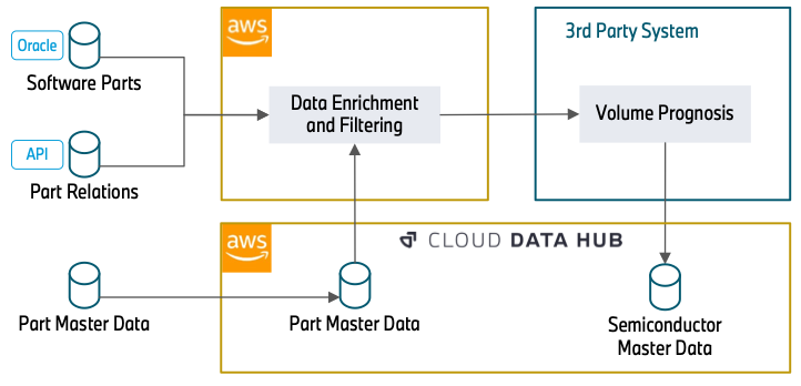
The data enrichment starts with an Oracle Database (Software Parts) that contains part numbers that are related to software. This can be the control unit of a headlight or a camera system for automated driving. Because semiconductors are the basis for running software, this database builds the foundation of our data processing.
In the next step, we use REST APIs (Part Relations) to enrich the data with further attributes. This includes how parts are related (for example, a specific control unit that will be installed into a headlight) and over which timespan a part number will be built into a vehicle. The knowledge about the part relations is essential to understand how a specific semiconductor, in this case the control unit, is relevant for a more general part, the headlight. The temporal information about the use of part numbers allows us to filter out outdated part numbers, which will not be used in the future and therefore have no relevance in the forecast.
The data (Part Master Data) can directly be consumed from the Cloud Data Hub. This database includes attributes about the status and material types of a part number. This information is required to filter out part numbers that we gathered in the previous steps but have no relevance for semiconductors. With the information that was gathered from the APIs, this data is also queried to extract further part numbers that weren’t ingested in the previous steps.
After data enrichment and filtering, a third-party system reads the filtered part data and enriches the semiconductor information. Subsequently, it adds the volume information of the components. Finally, it provides the overall semiconductor demand forecast centrally to the Cloud Data Hub.
Applied services
Our solution uses the serverless services AWS Glue and Amazon Simple Storage Service (Amazon S3) to run ETL (extract, transform, and load) workflows without managing an infrastructure. It also reduces the costs by paying only for the time jobs are running. The serverless approach fits our workflow’s schedule very well because we run the workload only once a week.
Because we’re using diverse data source systems as well as complex processing and aggregation, it’s important to decouple ETL jobs. This allows us to process each data source independently. We also split the data transformation into several modules (Data Aggregation, Data Filtering, and Data Preparation) to make the system more transparent and easier to maintain. This approach also helps in case of extending or modifying existing jobs.
Although each module is specific to a data source or a particular data transformation, we utilize reusable blocks inside of every job. This allows us to unify each type of operation and simplifies the procedure of adding new data sources and transformation steps in the future.
In our setup, we follow the security best practice of the least privilege principle, to ensure the information is protected from accidental or unnecessary access. Therefore, each module has AWS Identity and Access Management (IAM) roles with only the necessary permissions, namely access to only data sources and buckets the job deals with. For more information regarding security best practices, refer to Security best practices in IAM.
Solution overview
The following diagram shows the overall workflow where several AWS Glue jobs are interacting with each other sequentially.

As we mentioned earlier, we used the Cloud Data Hub, Oracle DB, and other data sources that we communicate with via the REST API. The first step of the solution is the Data Source Ingest module, which ingests the data from different data sources. For that purpose, AWS Glue jobs read information from different data sources and writes into the S3 source buckets. Ingested data is stored in the encrypted buckets, and keys are managed by AWS Key Management Service (AWS KMS).
After the Data Source Ingest step, intermediate jobs aggregate and enrich the tables with other data sources like components version and categories, model manufacture dates, and so on. Then they write them into the intermediate buckets in the Data Aggregation module, creating comprehensive and abundant data representation. Additionally, according to the business logic workflow, the Data Filtering and Data Preparation modules create the final master data table with only actual and production-relevant information.
The AWS Glue workflow manages all these ingestion jobs and filtering jobs end to end. An AWS Glue workflow schedule is configured weekly to run the workflow on Wednesdays. While the workflow is running, each job writes execution logs (info or error) into Amazon Simple Notification Service (Amazon SNS) and Amazon CloudWatch for monitoring purposes. Amazon SNS forwards the execution results to the monitoring tools, such as Mail, Teams, or Slack channels. In case of any error in the jobs, Amazon SNS also alerts the listeners about the job execution result to take action.
As the last step of the solution, the third-party system reads the master table from the prepared data bucket via Amazon Athena. After further data engineering steps like semiconductor information enrichment and volume information integration, the final master data asset is written into the Cloud Data Hub. With the data now provided in the Cloud Data Hub, other use cases can use this semiconductor master data without building several interfaces to different source systems.
Business outcome
The project results provide the BMW Group a substantial transparency about their semiconductor demand for their entire vehicle portfolio in the present and in the future. The creation of a database with that magnitude enables the BMW Group to establish even further use cases to the benefit of more supply chain transparency and clearer and deeper exchange with first-tier suppliers and semiconductor manufacturers. It helps not only to resolve the current demanding market situation, but also to be more resilient in the future. Therefore, it’s one major step to a digital, transparent supply chain.
Conclusion
This post describes how to analyze semiconductor demand from many data sources with big data jobs in an AWS Glue workflow. A serverless architecture with minimal diversity of services makes the code base and architecture simple to understand and maintain. To learn more about how to use AWS Glue workflows and jobs for serverless orchestration, visit the AWS Glue service page.
About the authors
 Maik Leuthold is a Project Lead at the BMW Group for advanced analytics in the business field of supply chain and procurement, and leads the digitalization strategy for the semiconductor management.
 Nick Harmening is an IT Project Lead at the BMW Group and an AWS certified Solutions Architect. He builds and operates cloud-native applications with a focus on data engineering and machine learning.
 Göksel Sarikaya is a Senior Cloud Application Architect at AWS Professional Services. He enables customers to design scalable, cost-effective, and competitive applications through the innovative production of the AWS platform. He helps them to accelerate customer and partner business outcomes during their digital transformation journey.
 Alexander Tselikov is a Data Architect at AWS Professional Services who is passionate about helping customers to build scalable data, analytics and ML solutions to enable timely insights and make critical business decisions.
 Rahul Shaurya is a Senior Big Data Architect at Amazon Web Services. He helps and works closely with customers building data platforms and analytical applications on AWS. Outside of work, Rahul loves taking long walks with his dog Barney.