Post Syndicated from Claire Given original https://www.raspberrypi.org/blog/astro-pi-computer-back-from-space-is-now-on-display-at-the-science-museum/
After seven successful years on the International Space Station, 250 vertical miles above our planet, the original two Astro Pi computers that we sent to the ISS to help young people run their code in space have been returned to Earth. From today, one of these Astro Pi computers will be displayed in the Science Museum, London. You can visit it in the new Engineers Gallery, which is dedicated to world-changing engineering innovations and the diverse and fascinating range of people behind them.
A challenge to inspire young people about space and computing
The original Astro Pis, nicknamed Izzy and Ed, have played a major part in feeding tens of thousands of young people’s understanding and passion for science, mathematics, engineering, computing, and coding. In their seven years on the International Space Station (ISS), Izzy and Ed had the job of running over 70,000 programs created by young people as part of the annual Astro Pi Challenge.
Nicki Ashworth, 21, took part in the first-ever Astro Pi challenge after hearing about the opportunity at a science fair: “I thought it sounded like an interesting project, and good practice for my programming skills. I was young and had no idea of the extent of the project and how much it would influence my future.”
Like many young people who have participated in the Astro Pi Challenge, Nicki credits the Astro Pi Challenge as an inspiration to learn more about space and programming, and to decide on a career path: “My experience with Astro Pi definitely helped to shape my future choices. I’m currently in my third year of a Mechanical Engineering degree at University of Southampton, specialising in Computational Engineering and Design. I’ve always loved programming, which is why I took part in the Astro Pi competition, but it led to a fascination with space. This encouraged me to look at engineering as a future, and led me to where I am today!”
In the beginning…
It all started in 2014, when we started collaborating with organisations including the UK Space Agency and European Space Agency (ESA) to fly two Astro Pi computers to the ISS for educational activities during the six-month Principia mission of British ESA astronaut Tim Peake.
The Astro Pi computers each consist of a Raspberry Pi computer integrated with a digital camera and an add-on board filled with environmental sensors, all enclosed in a protective aluminium flight case.
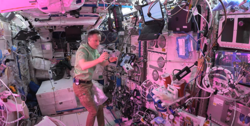
Commander Tim Peake, Britain’s first visitor to the ISS, accompanied the two first Astro Pi computers on the ISS. He used them to run experiments imagined, designed, and coded by school-age young people across the UK.
We held a competition in UK schools and coding clubs to invite young people to create experiments that could be run on the Astro Pis. Students conceived experiments and coded them in Python; we tested their Python programs and eventually picked seven to run on Izzy and Ed on the ISS.
The students’ experiments ranged from a simple but beautiful program to display the flag of the country over which the ISS was flying at a given time, to a reaction-time test for Tim Peake to measure his changing abilities across the six-month mission. The measurements from all the experiments were downloaded to Earth and analysed by the students.
“I still feel incredibly honoured to have competed in the very first [Astro Pi Challenge],” says Aaron Chamberlain, 18, who was 11 years old when he took part in the first-ever Astro Pi Challenge in 2015. “The experience was incredible and really cemented my enthusiasm for all things computing and coding. Finally looking at the photos the Raspberry Pi had taken of the astronauts floating 400 km above us was a feeling of awe that I will never forget.”
The next year, 2016, we expanded our partnership with ESA Education to be able to open up Astro Pi to young people across ESA Member states. The European Astro Pi Challenge has been going from strength to strength each year since, inspiring young people and adult mentors alike.
And today…
In 2021 we decided it was time to retire Izzy and Ed and replace them with upgraded Astro Pi computers with plenty of new and improved hardware, including a Raspberry Pi 4 Model B with 8 GB RAM.
Dave Honess, STEM Didactics Expert at the European Space Agency, was engineering lead at the Foundation for the first Astro Pi Challenge, and the return of the original hardware is a special event and moment of reflection for him: “It was a strange experience to open the box and hold the original Astro Pis again after all that time and distance they have travelled — literally billions of miles. Even though their mission is over, we will continue to learn from them with a tear-down analysis to find out if they have been affected by their time in space. Since Principia, I have watched the European Astro Pi Challenge grow with pride year on year, but I still feel very fortunate to have been there at the beginning.”
Thanks to the upgraded hardware, we are able to continue to grow the Astro Pi Challenge in collaboration with ESA Education. And each year it’s so exciting to see the creative and ingenious programs tens of thousands of young people from across Europe send us; 24,850 young people took part in the Challenge in the 2022/2023 cycle.
But how have Astro Pis Izzy and Ed fared in space over these seven years? Jonathan Bell, Principal Software Engineer at Raspberry Pi Limited, had a chance to find out first-hand: “I was lucky enough to have a look inside the returned Astro Pis. I was looking for the cosmetic effects of the unit being on the ISS for so long. On the inside they still look as pristine as when I assembled them! Barely a speck of dust on the internal boards, nor any signs that the external interface ports were worn from their years of use. A few dings and scrapes on the anodised exterior were all that I could see — and a missing joystick cap (as it turns out, hot-melt glue isn’t a permanent adhesive…). It was great to see that they still worked! It made me feel proud for what the team and the Astro Pi programme has achieved over the years. It’s good to have Izzy and Ed back!”

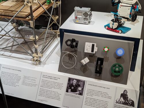
Visit the Science Museum to see an Astro Pi for yourself
The new Engineers Gallery in the Science Museum opens today and is free to visit. Astro Pi computer Izzy is among the amazing exhibits. Learn more at: sciencemuseum.org.uk/engineers
To find out more about the Astro Pi Challenge and how to get involved with your kids at home, your school, or your STEM or coding club, visit astro-pi.org.
The next round of the Challenge starts in September — sign up for news to be the first to hear when we launch it.
The post Welcome home! An original Astro Pi computer back from space is now on display at the Science Museum appeared first on Raspberry Pi Foundation.