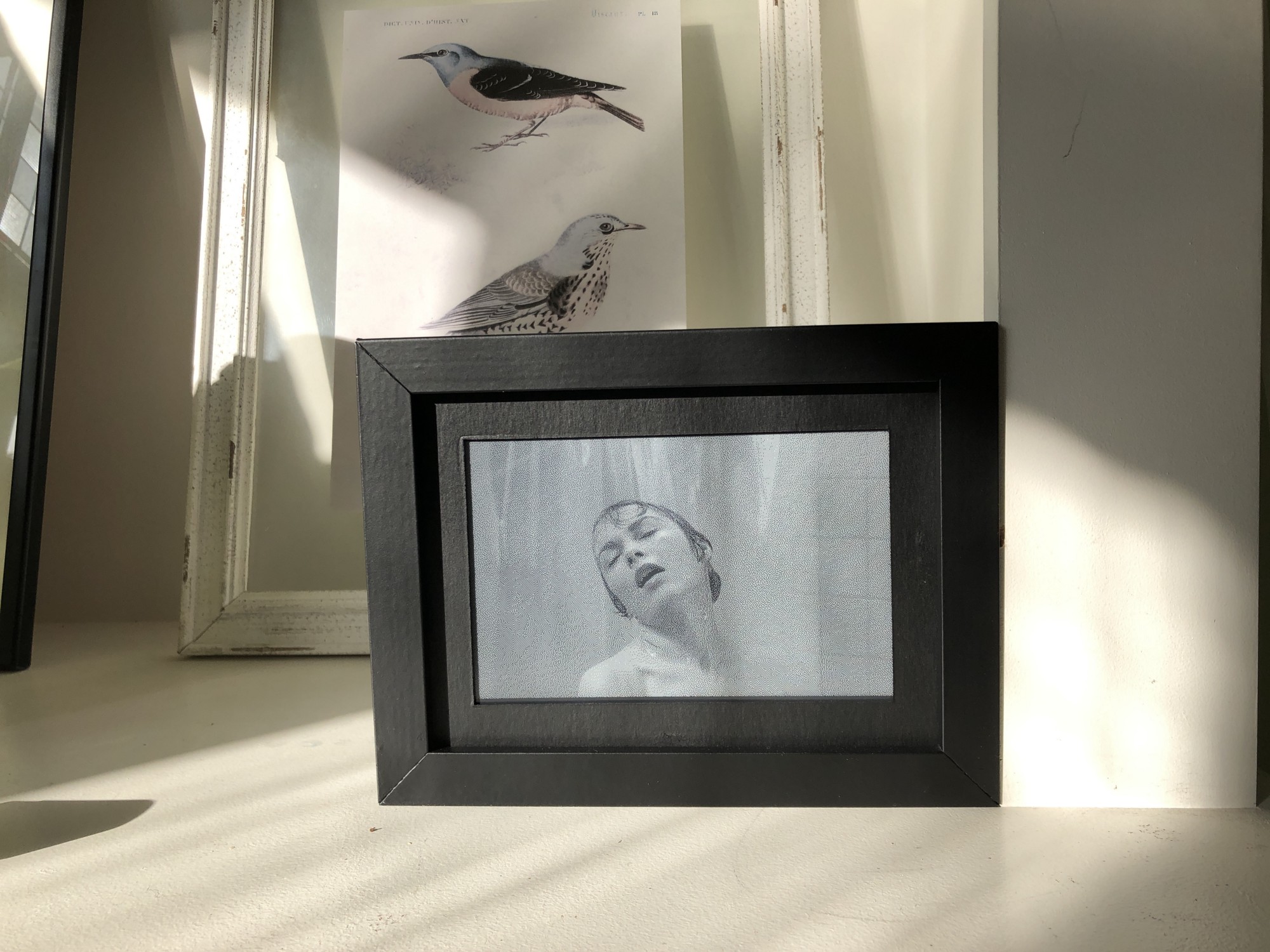
His creation plays films at about two minutes of screen time per 24 hours, taking a little under three months for a 110-minute film. Psycho played in a corner of his dining room for two months. The infamous shower scene lasted a day and a half.
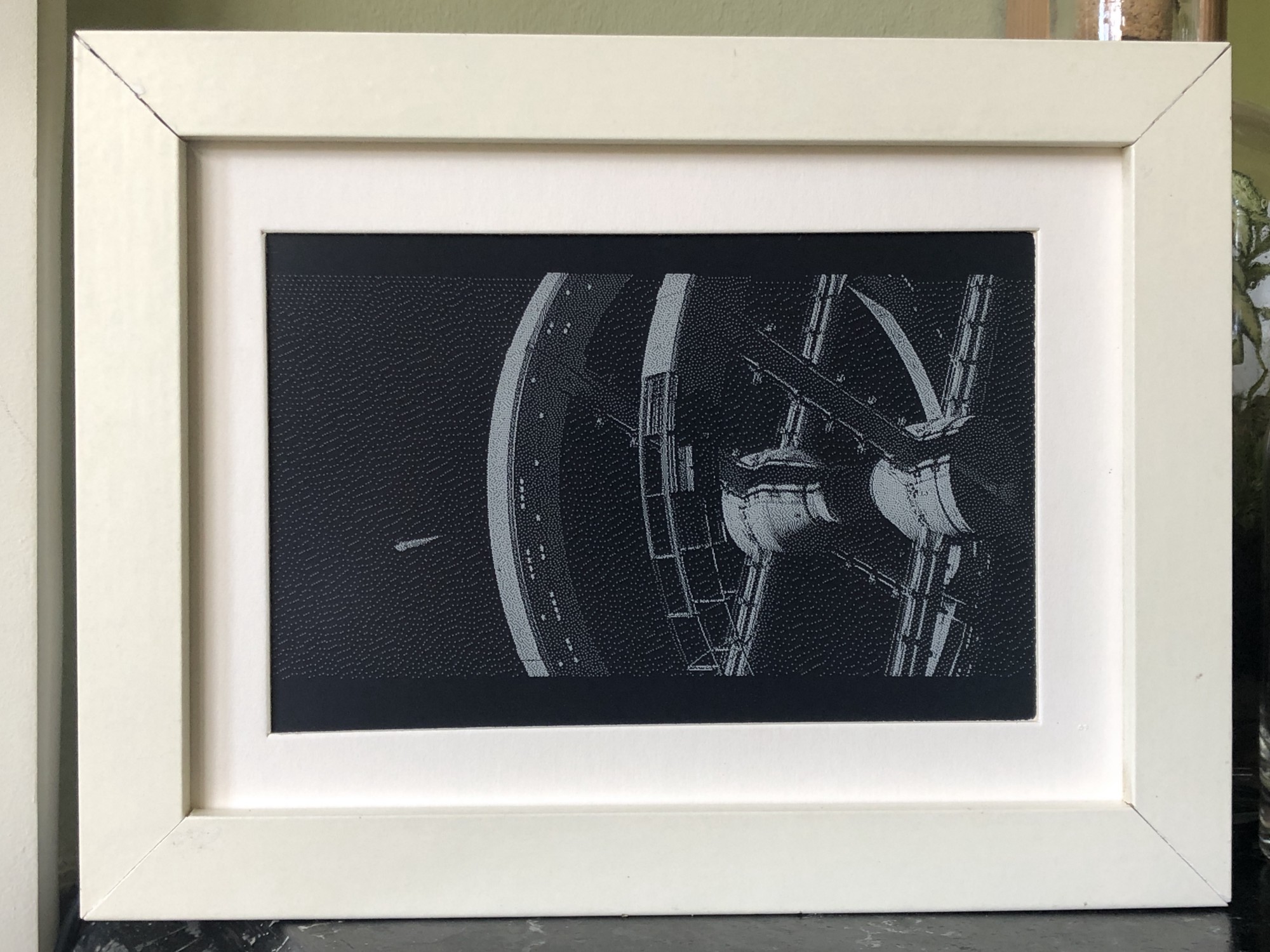
Tom enjoys the opportunity for close study of iconic filmmaking, but you might like this project for the living artwork angle. How cool would this be playing your favourite film onto a plain wall somewhere you can see it throughout the day?
The Raspberry Pi wearing its e-Paper HAT
Four simple steps
Luckily, this is a relatively simple project – no hardcore coding, no soldering required – with just four steps to follow if you’d like to recreate it:
Get the Raspberry Pi working in headless mode without a monitor, so you can upload files and run code
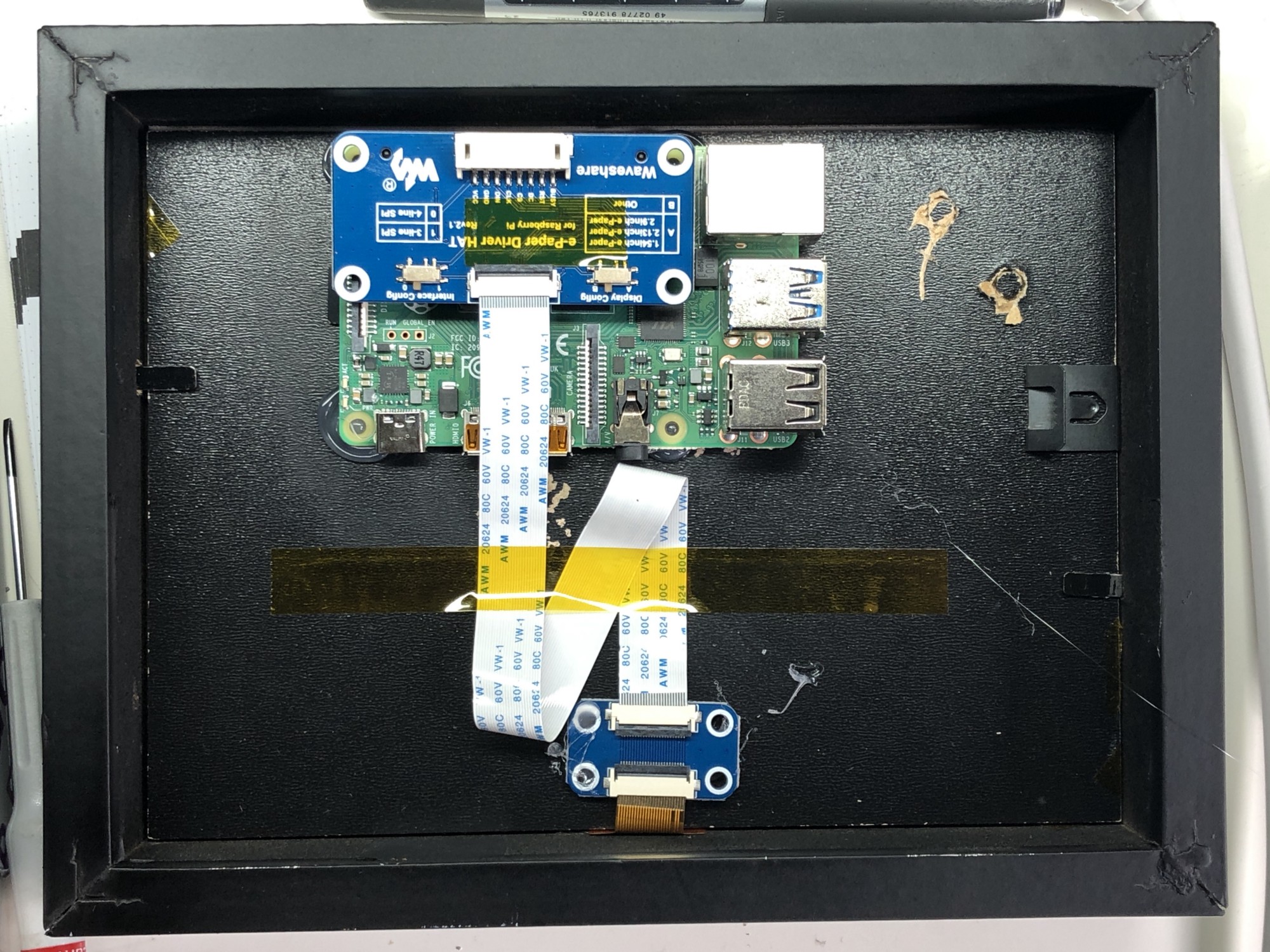
Connect to an e-paper display via an e-paper HAT (see above image; Tom is using this one) and install the driver code on the Raspberry Pi
Use Tom’s code to extract frames from a movie file, resize and dither those frames, display them on the screen, and keep track of progress through the film
Find some kind of frame to keep it all together (Tom went with a trusty IKEA number)
Living artwork: the Psycho shower scene playing alongside still artwork in Tom’s home
Affordably arty
The entire build cost £120 in total. Tom chose a 2GB Raspberry Pi 4 and a NOOBS 64gb SD Card, which he bought from Pimoroni, one of our approved resellers. NOOBS included almost all the libraries he needed for this project, which made life a lot easier.
His original post is a dream of a comprehensive walkthrough, including all the aforementioned code.
2001: A Space Odyssey would take months to play on Tom’s creation
Head to the comments section with your vote for the creepiest film to watch in ultra slow motion. I came over all peculiar imaging Jaws playing on my living room wall for months. Big bloody mouth opening slooooowly (pales), big bloody teeth clamping down slooooowly (heart palpitations). Yeah, not going to try that. Sorry Tom.
In the 1993 action movie Demolition Man, Sylvester Stallone stars as a 1990s cop transported to the near-future. Technology plays a central role in the film, often bemusing the lead character. In a memorable scene, he is repeatedly punished by a ticketing machine for using bad language (a violation of the verbal morality statute).
In the future of Demolition Man, an always-listening government machine detects every banned word and issues a fine in the form of a receipt from a wall-mounted printer. This tutorial shows you how to build your own version using Raspberry Pi, the Google Voice API, and a thermal printer. Not only can it replicate detecting banned words, but it also doubles as a handy voice-to-paper stenographer (if you want a more serious use).
Prepare the hardware
We built a full ‘boxed’ project, but you can keep it simple if you wish. Your Raspberry Pi needs a method for listening, speaking, and printing. The easiest solution is to use USB for all three.
To issue our receipts we used a thermal printer, the kind found in supermarket tills. This particular model is surprisingly versatile, handling text and graphics.
It takes standard 2.25-inch (57mm) receipt paper, available in rolls of 15 metres. When printing, it does draw a lot of current, so we advise using a separate power supply. Do not attempt to power it from your Raspberry Pi. You may need to fit a barrel connector and source a 5V/1.5A power supply. The printer uses a UART/TTL serial connection, which neatly fits on to the GPIO. Although the printer’s connection is listed as being 5V, it is in fact 3.3V, so it can be directly connected to the ground, TX, and RX pins (physical pins 6, 8, 10) on the GPIO.
Install and configure Raspbian
Get yourself a copy of Raspbian Buster Lite and burn it to a microSD card using a tool like Etcher. You can use the full version of Buster if you wish. Perform the usual steps of getting a wireless connection and then updating to the latest version using sudo apt update && sudo apt -y upgrade. From a command prompt, run sudo raspi-config and go to ‘Interfacing options’, then ‘Enable serial’. When asked if you would like the login shell to be accessible, respond ‘No’. To the next question, ‘Would you like the serial port hardware to be enabled?’, reply ‘Yes’. Now reboot your Raspberry Pi.
Test the printer
Make sure the printer is up and running. Double-check you’ve connected the header to the GPIO correctly and power up the printer. The LED on the printer should flash every few seconds. Load in the paper and make sure it’s feeding correctly. We can talk to the printer directly, but the Python ‘thermalprinter‘ library makes coding for it so much easier. To install the library:
Create a file called printer.py and enter in the code in the relevant listing. Run the code using:
python3 printer.py
If you got a nice welcoming message, your printer is all set to go.
Test the microphone
Once your microphone is connected to Raspberry Pi, check the settings by running:
alsamixer
This utility configures your various sound devices. Press F4 to enter ‘capture’ mode (microphones), then press F6 and select your device from the list. Make sure the microphone is not muted (M key) and the levels are high, but not in the red zone.
Back at the command line, run this command:
arecord -l
This shows a list of available recording devices, one of which will be your microphone. Make a note of the card number and subdevice number.
If your card and subdevice numbers were not ‘0,1’, you’ll need to change the device parameter in the above command.
Say a few words, then use CTRL+C to stop recording. Check the playback with:
aplay test.wav
Choose your STT provider
STT means speech to text and refers to the code that can take an audio recording and return recognised speech as plain text. Many solutions are available and can be used in this project. For the greatest accuracy, we’re going to use Google Voice API. Rather than doing the complex processing locally, a compressed version of the sound file is uploaded to Google Cloud and the text returned. However, this does mean Google gets a copy of everything ‘heard’ by the project. If this isn’t for you, take a look at Jasper, an open-source alternative that supports local processing.
Create your Google project
To use the Google Cloud API, you’ll need a Google account. Log in to the API Console at console.developers.google.com. We need to create a project here. Next to ‘Google APIs’, click the drop-down menu, then ‘New Project’. Give it a name. You’ll be prompted to enable APIs for the project. Click the link, then search for ‘speech’. Click on ‘Cloud Speech-to-Text API’, then ‘Enable’. At this point you may be prompted for billing information. Don’t worry, you can have up to 60 minutes of audio transcribed for free each month.
Get your credentials
Once the Speech API is enabled, the screen will refresh and you’ll be prompted to create credentials. This is the info our code needs to be granted access to the speech-to-text API. Click on ‘Create Credentials’ and on the next screen select ‘Cloud Speech-to-text API’. You’re asked if you’re planning to use the Compute Engine; select ‘no’. Now create a ‘service account’. Give it a different name from the one used earlier, change the role to ‘Project Owner’, leave the type of file as ‘JSON’, and click ‘Continue’. A file will be downloaded to your computer; transfer this to your Raspberry Pi.
Test Google recognition
When you’re happy with the recording levels, record a short piece of speech and save it as test.wav. We’ll send this to Google and check our access to the API is working. Install the Google Speech-To-Text Python library:
(Don’t forget to replace [FILE_NAME] with the actual name of the JSON file).
Using a text editor, create a file called speech_to_text.py and enter the code from the relevant listing. Then run it:
python3 speech_to_text.py
If everything is working correctly, you’ll get a text transcript back within a few seconds.
Live transcription
Amazingly, Google’s speech-to-text service can also support streaming recognition, so rather than capture-then-process, the audio can be sent as a stream, and a HTTP stream of the recognised text comes back. When there is a pause in the speech, the results are finalised, so then we can send the results to the printer. If all the code you’ve entered so far is running correctly, all you need to do is download the stenographer.py script and start it using:
python3 stenographer.py
You are limited on how long you can record for, but this could be coupled with a ‘push to talk’ button so you can make notes using only your voice!
Banned word game
Back to Demolition Man. We need to make an alarm sound, so install a speaker (a passive one that connects to the 3.5mm jack is ideal; we used a Pimoroni Speaker pHAT). Download the banned.py code and edit it in your favourite text editor. At the top is a list of words. You can change this to anything you like (but don’t offend anyone!). In our list, the system is listening for a few mild naughty words. In the event anyone mentions one, a buzzer will sound and a fine will be printed.
Make up your list and start the game by running:
python3 banned.py
Now try one of your banned words.
Package it up
Whatever you decide to use this project for, why not finish it up with a 3D-printed case so you package up the printer and Raspberry Pi with the recording and playback devices and create a portable unit? Ideal for pranking friends or taking notes on the move!
See if you can invent any other games using voice recognition, or investigate the graphics capability of the printer. Add a Raspberry Pi Camera Module for retro black and white photos. Combine it with facial recognition to print out an ID badge just using someone’s face. Over to you.
The MagPi magazine issue 84
This project was created by PJ Evans for The MagPi magazine issue 84, available now online, from your local newsagents, or as a free download from The MagPi magazine website.
If, like us, you’ve been bingeflixing your way through Netflix’s new show, Lost in Space, you may have noticed a Raspberry Pi being used as futuristic space tech.
Danger, Will Robinson, that probably won’t work
This isn’t the first time a Pi has been used as a film or television prop. From Mr. Robot and Disney Pixar’s Big Hero 6 to Mr. Robot, Sense8, and Mr. Robot, our humble little computer has become quite the celeb.
Raspberry Pi Spy has been working hard to locate and document the appearance of the Raspberry Pi in some of our favourite shows and movies. He’s created this video covering 2010-2017:
Since 2012 the Raspberry Pi single board computer has appeared in a number of movies and TV shows. This video is a run through of those appearances where the Pi has been used as a prop.
For 2018 appearances and beyond, you can find a full list on the Raspberry Pi Spy website. If you’ve spotted an appearance that’s not on the list, tell us in the comments!
AWS Glue provides enhanced support for working with datasets that are organized into Hive-style partitions. AWS Glue crawlers automatically identify partitions in your Amazon S3 data. The AWS Glue ETL (extract, transform, and load) library natively supports partitions when you work with DynamicFrames. DynamicFrames represent a distributed collection of data without requiring you to specify a schema. You can now push down predicates when creating DynamicFrames to filter out partitions and avoid costly calls to S3. We have also added support for writing DynamicFrames directly into partitioned directories without converting them to Apache Spark DataFrames.
Partitioning has emerged as an important technique for organizing datasets so that they can be queried efficiently by a variety of big data systems. Data is organized in a hierarchical directory structure based on the distinct values of one or more columns. For example, you might decide to partition your application logs in Amazon S3 by date—broken down by year, month, and day. Files corresponding to a single day’s worth of data would then be placed under a prefix such as s3://my_bucket/logs/year=2018/month=01/day=23/.
Systems like Amazon Athena, Amazon Redshift Spectrum, and now AWS Glue can use these partitions to filter data by value without making unnecessary calls to Amazon S3. This can significantly improve the performance of applications that need to read only a few partitions.
In this post, we show you how to efficiently process partitioned datasets using AWS Glue. First, we cover how to set up a crawler to automatically scan your partitioned dataset and create a table and partitions in the AWS Glue Data Catalog. Then, we introduce some features of the AWS Glue ETL library for working with partitioned data. You can now filter partitions using SQL expressions or user-defined functions to avoid listing and reading unnecessary data from Amazon S3. We’ve also added support in the ETL library for writing AWS Glue DynamicFrames directly into partitions without relying on Spark SQL DataFrames.
Let’s get started!
Crawling partitioned data
In this example, we use the same GitHub archive dataset that we introduced in a previous post about Scala support in AWS Glue. This data, which is publicly available from the GitHub archive, contains a JSON record for every API request made to the GitHub service. A sample dataset containing one month of activity from January 2017 is available at the following location:
Here you can replace <region> with the AWS Region in which you are working, for example, us-east-1. This dataset is partitioned by year, month, and day, so an actual file will be at a path like the following:
To crawl this data, you can either follow the instructions in the AWS Glue Developer Guide or use the provided AWS CloudFormation template. This template creates a stack that contains the following:
An IAM role with permissions to access AWS Glue resources
A database in the AWS Glue Data Catalog named githubarchive_month
A crawler set up to crawl the GitHub dataset
An AWS Glue development endpoint (which is used in the next section to transform the data)
To run this template, you must provide an S3 bucket and prefix where you can write output data in the next section. The role that this template creates will have permission to write to this bucket only. You also need to provide a public SSH key for connecting to the development endpoint. For more information about creating an SSH key, see our Development Endpoint tutorial. After you create the AWS CloudFormation stack, you can run the crawler from the AWS Glue console.
In addition to inferring file types and schemas, crawlers automatically identify the partition structure of your dataset and populate the AWS Glue Data Catalog. This ensures that your data is correctly grouped into logical tables and makes the partition columns available for querying in AWS Glue ETL jobs or query engines like Amazon Athena.
After you crawl the table, you can view the partitions by navigating to the table in the AWS Glue console and choosing View partitions. The partitions should look like the following:
For partitioned paths in Hive-style of the form key=val, crawlers automatically populate the column name. In this case, because the GitHub data is stored in directories of the form 2017/01/01, the crawlers use default names like partition_0, partition_1, and so on. You can easily change these names on the AWS Glue console: Navigate to the table, choose Edit schema, and rename partition_0 to year, partition_1 to month, and partition_2 to day:
Now that you’ve crawled the dataset and named your partitions appropriately, let’s see how to work with partitioned data in an AWS Glue ETL job.
Transforming and filtering the data
To get started with the AWS Glue ETL libraries, you can use an AWS Glue development endpoint and an Apache Zeppelin notebook. AWS Glue development endpoints provide an interactive environment to build and run scripts using Apache Spark and the AWS Glue ETL library. They are great for debugging and exploratory analysis, and can be used to develop and test scripts before migrating them to a recurring job.
If you ran the AWS CloudFormation template in the previous section, then you already have a development endpoint named partition-endpoint in your account. Otherwise, you can follow the instructions in this development endpoint tutorial. In either case, you need to set up an Apache Zeppelin notebook, either locally, or on an EC2 instance. You can find more information about development endpoints and notebooks in the AWS Glue Developer Guide.
The following examples are all written in the Scala programming language, but they can all be implemented in Python with minimal changes.
Reading a partitioned dataset
To get started, let’s read the dataset and see how the partitions are reflected in the schema. First, you import some classes that you will need for this example and set up a GlueContext, which is the main class that you will use to read and write data.
Execute the following in a Zeppelin paragraph, which is a unit of executable code:
%spark
import com.amazonaws.services.glue.DynamicFrame import com.amazonaws.services.glue.DynamicRecord
import com.amazonaws.services.glue.GlueContext
import com.amazonaws.services.glue.util.JsonOptions import org.apache.spark.SparkContext
import java.util.Calendar
import java.util.GregorianCalendar
import scala.collection.JavaConversions._
@transient val spark: SparkContext = SparkContext.getOrCreate()
val glueContext: GlueContext = new GlueContext(spark)
This is straightforward with two caveats: First, each paragraph must start with the line %spark to indicate that the paragraph is Scala. Second, the spark variable must be marked @transient to avoid serialization issues. This is only necessary when running in a Zeppelin notebook.
Next, read the GitHub data into a DynamicFrame, which is the primary data structure that is used in AWS Glue scripts to represent a distributed collection of data. A DynamicFrame is similar to a Spark DataFrame, except that it has additional enhancements for ETL transformations. DynamicFrames are discussed further in the post AWS Glue Now Supports Scala Scripts, and in the AWS Glue API documentation.
The following snippet creates a DynamicFrame by referencing the Data Catalog table that you just crawled and then prints the schema:
%spark
val githubEvents: DynamicFrame = glueContext.getCatalogSource(
database = "githubarchive_month",
tableName = "data"
).getDynamicFrame()
githubEvents.schema.asFieldList.foreach { field =>
println(s"${field.getName}: ${field.getType.getType.getName}")
}
You could also print the full schema using githubEvents.printSchema(). But in this case, the full schema is quite large, so I’ve printed only the top-level columns. This paragraph takes about 5 minutes to run on a standard size AWS Glue development endpoint. After it runs, you should see the following output:
Note that the partition columns year, month, and day were automatically added to each record.
Filtering by partition columns
One of the primary reasons for partitioning data is to make it easier to operate on a subset of the partitions, so now let’s see how to filter data by the partition columns. In particular, let’s find out what people are building in their free time by looking at GitHub activity on the weekends. One way to accomplish this is to use the filter transformation on the githubEvents DynamicFrame that you created earlier to select the appropriate events:
%spark
def filterWeekend(rec: DynamicRecord): Boolean = {
def getAsInt(field: String): Int = {
rec.getField(field) match {
case Some(strVal: String) => strVal.toInt
// The filter transformation will catch exceptions and mark the record as an error.
case _ => throw new IllegalArgumentException(s"Unable to extract field $field")
}
}
val (year, month, day) = (getAsInt("year"), getAsInt("month"), getAsInt("day"))
val cal = new GregorianCalendar(year, month - 1, day) // Calendar months start at 0.
val dayOfWeek = cal.get(Calendar.DAY_OF_WEEK)
dayOfWeek == Calendar.SATURDAY || dayOfWeek == Calendar.SUNDAY
}
val filteredEvents = githubEvents.filter(filterWeekend)
filteredEvents.count
This snippet defines the filterWeekend function that uses the Java Calendar class to identify those records where the partition columns (year, month, and day) fall on a weekend. If you run this code, you see that there were 6,303,480 GitHub events falling on the weekend in January 2017, out of a total of 29,160,561 events. This seems reasonable—about 22 percent of the events fell on the weekend, and about 29 percent of the days that month fell on the weekend (9 out of 31). So people are using GitHub slightly less on the weekends, but there is still a lot of activity!
Predicate pushdowns for partition columns
The main downside to using the filter transformation in this way is that you have to list and read all files in the entire dataset from Amazon S3 even though you need only a small fraction of them. This is manageable when dealing with a single month’s worth of data. But as you try to process more data, you will spend an increasing amount of time reading records only to immediately discard them.
To address this issue, we recently released support for pushing down predicates on partition columns that are specified in the AWS Glue Data Catalog. Instead of reading the data and filtering the DynamicFrame at executors in the cluster, you apply the filter directly on the partition metadata available from the catalog. Then you list and read only the partitions from S3 that you need to process.
To accomplish this, you can specify a Spark SQL predicate as an additional parameter to the getCatalogSource method. This predicate can be any SQL expression or user-defined function as long as it uses only the partition columns for filtering. Remember that you are applying this to the metadata stored in the catalog, so you don’t have access to other fields in the schema.
The following snippet shows how to use this functionality to read only those partitions occurring on a weekend:
%spark
val partitionPredicate =
"date_format(to_date(concat(year, '-', month, '-', day)), 'E') in ('Sat', 'Sun')"
val pushdownEvents = glueContext.getCatalogSource(
database = "githubarchive_month",
tableName = "data",
pushDownPredicate = partitionPredicate).getDynamicFrame()
Here you use the SparkSQL string concat function to construct a date string. You use the to_date function to convert it to a date object, and the date_format function with the ‘E’ pattern to convert the date to a three-character day of the week (for example, Mon, Tue, and so on). For more information about these functions, Spark SQL expressions, and user-defined functions in general, see the Spark SQL documentation and list of functions.
Note that the pushdownPredicate parameter is also available in Python. The corresponding call in Python is as follows:
You can observe the performance impact of pushing down predicates by looking at the execution time reported for each Zeppelin paragraph. The initial approach using a Scala filter function took 2.5 minutes:
Because the version using a pushdown lists and reads much less data, it takes only 24 seconds to complete, a 5X improvement!
Of course, the exact benefit that you see depends on the selectivity of your filter. The more partitions that you exclude, the more improvement you will see.
In addition to Hive-style partitioning for Amazon S3 paths, Parquet and ORC file formats further partition each file into blocks of data that represent column values. Each block also stores statistics for the records that it contains, such as min/max for column values. AWS Glue supports pushdown predicates for both Hive-style partitions and block partitions in these formats. While reading data, it prunes unnecessary S3 partitions and also skips the blocks that are determined unnecessary to be read by column statistics in Parquet and ORC formats.
Additional transformations
Now that you’ve read and filtered your dataset, you can apply any additional transformations to clean or modify the data. For example, you could augment it with sentiment analysis as described in the previous AWS Glue post.
To keep things simple, you can just pick out some columns from the dataset using the ApplyMapping transformation:
ApplyMapping is a flexible transformation for performing projection and type-casting. In this example, we use it to unnest several fields, such as actor.login, which we map to the top-level actor field. We also cast the id column to a long and the partition columns to integers.
Writing out partitioned data
The final step is to write out your transformed dataset to Amazon S3 so that you can process it with other systems like Amazon Athena. By default, when you write out a DynamicFrame, it is not partitioned—all the output files are written at the top level under the specified output path. Until recently, the only way to write a DynamicFrame into partitions was to convert it into a Spark SQL DataFrame before writing. We are excited to share that DynamicFrames now support native partitioning by a sequence of keys.
You can accomplish this by passing the additional partitionKeys option when creating a sink. For example, the following code writes out the dataset that you created earlier in Parquet format to S3 in directories partitioned by the type field.
Here, $outpath is a placeholder for the base output path in S3. The partitionKeys parameter can also be specified in Python in the connection_options dict:
When you execute this write, the type field is removed from the individual records and is encoded in the directory structure. To demonstrate this, you can list the output path using the aws s3 ls command from the AWS CLI:
PRE type=CommitCommentEvent/
PRE type=CreateEvent/
PRE type=DeleteEvent/
PRE type=ForkEvent/
PRE type=GollumEvent/
PRE type=IssueCommentEvent/
PRE type=IssuesEvent/
PRE type=MemberEvent/
PRE type=PublicEvent/
PRE type=PullRequestEvent/
PRE type=PullRequestReviewCommentEvent/
PRE type=PushEvent/
PRE type=ReleaseEvent/
PRE type=WatchEvent/
As expected, there is a partition for each distinct event type. In this example, we partitioned by a single value, but this is by no means required. For example, if you want to preserve the original partitioning by year, month, and day, you could simply set the partitionKeys option to be Seq(“year”, “month”, “day”).
Conclusion
In this post, we showed you how to work with partitioned data in AWS Glue. Partitioning is a crucial technique for getting the most out of your large datasets. Many tools in the AWS big data ecosystem, including Amazon Athena and Amazon Redshift Spectrum, take advantage of partitions to accelerate query processing. AWS Glue provides mechanisms to crawl, filter, and write partitioned data so that you can structure your data in Amazon S3 however you want, to get the best performance out of your big data applications.
Ben Sowell is a senior software development engineer at AWS Glue. He has worked for more than 5 years on ETL systems to help users unlock the potential of their data. In his free time, he enjoys reading and exploring the Bay Area.
Mohit Saxena is a senior software development engineer at AWS Glue. His passion is building scalable distributed systems for efficiently managing data on cloud. He also enjoys watching movies and reading about the latest technology.
Grab your Raspberry Pi, everyone — we’re going on an Easter egg hunt, and all of you are invited!
When they’re not chocolate, Easter eggs are hidden content in movies, games, DVD menus, and computers. So open a terminal window and try the following:
1. A little attitude
Type aptitude moo into the terminal window and press Enter. Now type aptitude -v moo. Keep adding v’s, like this: aptitude -vv moo
2. Party
Addicted to memes? Type curl parrot.live into your window!
3. In a galaxy far, far away…
You’ll need to install telnet for this one: start by typing sudo apt-get install telnet into the terminal. Once it’s installed, enter telnet towel.blinkenlights.nl
4. Pinout
Type pinout into the window to see a handy GPIO pinout diagram for your Pi. Ideal for physical digital making projects!
5. Demo programs
Easter egg-ish: you can try out various demo programs on your Raspberry Pi, such as 1080p video playback and spinning teapots.
Any more?
There’s lots of fun to be had in the terminal of a Raspberry Pi. Do you know any other fun Easter eggs? Share them in the comments!
In this blog post, I will show how you can perform unit testing as a part of your AWS CodeStar project. AWS CodeStar helps you quickly develop, build, and deploy applications on AWS. With AWS CodeStar, you can set up your continuous delivery (CD) toolchain and manage your software development from one place.
Because unit testing tests individual units of application code, it is helpful for quickly identifying and isolating issues. As a part of an automated CI/CD process, it can also be used to prevent bad code from being deployed into production.
Many of the AWS CodeStar project templates come preconfigured with a unit testing framework so that you can start deploying your code with more confidence. The unit testing is configured to run in the provided build stage so that, if the unit tests do not pass, the code is not deployed. For a list of AWS CodeStar project templates that include unit testing, see AWS CodeStar Project Templates in the AWS CodeStar User Guide.
The scenario
As a big fan of superhero movies, I decided to list my favorites and ask my friends to vote on theirs by using a WebService endpoint I created. The example I use is a Python web service running on AWS Lambda with AWS CodeCommit as the code repository. CodeCommit is a fully managed source control system that hosts Git repositories and works with all Git-based tools.
Here’s how you can create the WebService endpoint:
Sign in to the AWS CodeStar console. Choose Start a project, which will take you to the list of project templates.
For code edits I will choose AWS Cloud9, which is a cloud-based integrated development environment (IDE) that you use to write, run, and debug code.
Here are the other tasks required by my scenario:
Create a database table where the votes can be stored and retrieved as needed.
Update the logic in the Lambda function that was created for posting and getting the votes.
Update the unit tests (of course!) to verify that the logic works as expected.
For a database table, I’ve chosen Amazon DynamoDB, which offers a fast and flexible NoSQL database.
Getting set up on AWS Cloud9
From the AWS CodeStar console, go to the AWS Cloud9 console, which should take you to your project code. I will open up a terminal at the top-level folder under which I will set up my environment and required libraries.
Use the following command to set the PYTHONPATH environment variable on the terminal.
You should now be able to use the following command to execute the unit tests in your project.
python -m unittest discover vote-your-movie/tests
Start coding
Now that you have set up your local environment and have a copy of your code, add a DynamoDB table to the project by defining it through a template file. Open template.yml, which is the Serverless Application Model (SAM) template file. This template extends AWS CloudFormation to provide a simplified way of defining the Amazon API Gateway APIs, AWS Lambda functions, and Amazon DynamoDB tables required by your serverless application.
AWSTemplateFormatVersion: 2010-09-09
Transform:
- AWS::Serverless-2016-10-31
- AWS::CodeStar
Parameters:
ProjectId:
Type: String
Description: CodeStar projectId used to associate new resources to team members
Resources:
# The DB table to store the votes.
MovieVoteTable:
Type: AWS::Serverless::SimpleTable
Properties:
PrimaryKey:
# Name of the "Candidate" is the partition key of the table.
Name: Candidate
Type: String
# Creating a new lambda function for retrieving and storing votes.
MovieVoteLambda:
Type: AWS::Serverless::Function
Properties:
Handler: index.handler
Runtime: python3.6
Environment:
# Setting environment variables for your lambda function.
Variables:
TABLE_NAME: !Ref "MovieVoteTable"
TABLE_REGION: !Ref "AWS::Region"
Role:
Fn::ImportValue:
!Join ['-', [!Ref 'ProjectId', !Ref 'AWS::Region', 'LambdaTrustRole']]
Events:
GetEvent:
Type: Api
Properties:
Path: /
Method: get
PostEvent:
Type: Api
Properties:
Path: /
Method: post
We’ll use Python’s boto3 library to connect to AWS services. And we’ll use Python’s mock library to mock AWS service calls for our unit tests. Use the following command to install these libraries:
pip install --upgrade boto3 mock -t .
Add these libraries to the buildspec.yml, which is the YAML file that is required for CodeBuild to execute.
version: 0.2
phases:
install:
commands:
# Upgrade AWS CLI to the latest version
- pip install --upgrade awscli boto3 mock
pre_build:
commands:
# Discover and run unit tests in the 'tests' directory. For more information, see <https://docs.python.org/3/library/unittest.html#test-discovery>
- python -m unittest discover tests
build:
commands:
# Use AWS SAM to package the application by using AWS CloudFormation
- aws cloudformation package --template template.yml --s3-bucket $S3_BUCKET --output-template template-export.yml
artifacts:
type: zip
files:
- template-export.yml
Open the index.py where we can write the simple voting logic for our Lambda function.
import json
import datetime
import boto3
import os
table_name = os.environ['TABLE_NAME']
table_region = os.environ['TABLE_REGION']
VOTES_TABLE = boto3.resource('dynamodb', region_name=table_region).Table(table_name)
CANDIDATES = {"A": "Black Panther", "B": "Captain America: Civil War", "C": "Guardians of the Galaxy", "D": "Thor: Ragnarok"}
def handler(event, context):
if event['httpMethod'] == 'GET':
resp = VOTES_TABLE.scan()
return {'statusCode': 200,
'body': json.dumps({item['Candidate']: int(item['Votes']) for item in resp['Items']}),
'headers': {'Content-Type': 'application/json'}}
elif event['httpMethod'] == 'POST':
try:
body = json.loads(event['body'])
except:
return {'statusCode': 400,
'body': 'Invalid input! Expecting a JSON.',
'headers': {'Content-Type': 'application/json'}}
if 'candidate' not in body:
return {'statusCode': 400,
'body': 'Missing "candidate" in request.',
'headers': {'Content-Type': 'application/json'}}
if body['candidate'] not in CANDIDATES.keys():
return {'statusCode': 400,
'body': 'You must vote for one of the following candidates - {}.'.format(get_allowed_candidates()),
'headers': {'Content-Type': 'application/json'}}
resp = VOTES_TABLE.update_item(
Key={'Candidate': CANDIDATES.get(body['candidate'])},
UpdateExpression='ADD Votes :incr',
ExpressionAttributeValues={':incr': 1},
ReturnValues='ALL_NEW'
)
return {'statusCode': 200,
'body': "{} now has {} votes".format(CANDIDATES.get(body['candidate']), resp['Attributes']['Votes']),
'headers': {'Content-Type': 'application/json'}}
def get_allowed_candidates():
l = []
for key in CANDIDATES:
l.append("'{}' for '{}'".format(key, CANDIDATES.get(key)))
return ", ".join(l)
What our code basically does is take in the HTTPS request call as an event. If it is an HTTP GET request, it gets the votes result from the table. If it is an HTTP POST request, it sets a vote for the candidate of choice. We also validate the inputs in the POST request to filter out requests that seem malicious. That way, only valid calls are stored in the table.
In the example code provided, we use a CANDIDATES variable to store our candidates, but you can store the candidates in a JSON file and use Python’s json library instead.
Let’s update the tests now. Under the tests folder, open the test_handler.py and modify it to verify the logic.
import os
# Some mock environment variables that would be used by the mock for DynamoDB
os.environ['TABLE_NAME'] = "MockHelloWorldTable"
os.environ['TABLE_REGION'] = "us-east-1"
# The library containing our logic.
import index
# Boto3's core library
import botocore
# For handling JSON.
import json
# Unit test library
import unittest
## Getting StringIO based on your setup.
try:
from StringIO import StringIO
except ImportError:
from io import StringIO
## Python mock library
from mock import patch, call
from decimal import Decimal
@patch('botocore.client.BaseClient._make_api_call')
class TestCandidateVotes(unittest.TestCase):
## Test the HTTP GET request flow.
## We expect to get back a successful response with results of votes from the table (mocked).
def test_get_votes(self, boto_mock):
# Input event to our method to test.
expected_event = {'httpMethod': 'GET'}
# The mocked values in our DynamoDB table.
items_in_db = [{'Candidate': 'Black Panther', 'Votes': Decimal('3')},
{'Candidate': 'Captain America: Civil War', 'Votes': Decimal('8')},
{'Candidate': 'Guardians of the Galaxy', 'Votes': Decimal('8')},
{'Candidate': "Thor: Ragnarok", 'Votes': Decimal('1')}
]
# The mocked DynamoDB response.
expected_ddb_response = {'Items': items_in_db}
# The mocked response we expect back by calling DynamoDB through boto.
response_body = botocore.response.StreamingBody(StringIO(str(expected_ddb_response)),
len(str(expected_ddb_response)))
# Setting the expected value in the mock.
boto_mock.side_effect = [expected_ddb_response]
# Expecting that there would be a call to DynamoDB Scan function during execution with these parameters.
expected_calls = [call('Scan', {'TableName': os.environ['TABLE_NAME']})]
# Call the function to test.
result = index.handler(expected_event, {})
# Run unit test assertions to verify the expected calls to mock have occurred and verify the response.
assert result.get('headers').get('Content-Type') == 'application/json'
assert result.get('statusCode') == 200
result_body = json.loads(result.get('body'))
# Verifying that the results match to that from the table.
assert len(result_body) == len(items_in_db)
for i in range(len(result_body)):
assert result_body.get(items_in_db[i].get("Candidate")) == int(items_in_db[i].get("Votes"))
assert boto_mock.call_count == 1
boto_mock.assert_has_calls(expected_calls)
## Test the HTTP POST request flow that places a vote for a selected candidate.
## We expect to get back a successful response with a confirmation message.
def test_place_valid_candidate_vote(self, boto_mock):
# Input event to our method to test.
expected_event = {'httpMethod': 'POST', 'body': "{\"candidate\": \"D\"}"}
# The mocked response in our DynamoDB table.
expected_ddb_response = {'Attributes': {'Candidate': "Thor: Ragnarok", 'Votes': Decimal('2')}}
# The mocked response we expect back by calling DynamoDB through boto.
response_body = botocore.response.StreamingBody(StringIO(str(expected_ddb_response)),
len(str(expected_ddb_response)))
# Setting the expected value in the mock.
boto_mock.side_effect = [expected_ddb_response]
# Expecting that there would be a call to DynamoDB UpdateItem function during execution with these parameters.
expected_calls = [call('UpdateItem', {
'TableName': os.environ['TABLE_NAME'],
'Key': {'Candidate': 'Thor: Ragnarok'},
'UpdateExpression': 'ADD Votes :incr',
'ExpressionAttributeValues': {':incr': 1},
'ReturnValues': 'ALL_NEW'
})]
# Call the function to test.
result = index.handler(expected_event, {})
# Run unit test assertions to verify the expected calls to mock have occurred and verify the response.
assert result.get('headers').get('Content-Type') == 'application/json'
assert result.get('statusCode') == 200
assert result.get('body') == "{} now has {} votes".format(
expected_ddb_response['Attributes']['Candidate'],
expected_ddb_response['Attributes']['Votes'])
assert boto_mock.call_count == 1
boto_mock.assert_has_calls(expected_calls)
## Test the HTTP POST request flow that places a vote for an non-existant candidate.
## We expect to get back a successful response with a confirmation message.
def test_place_invalid_candidate_vote(self, boto_mock):
# Input event to our method to test.
# The valid IDs for the candidates are A, B, C, and D
expected_event = {'httpMethod': 'POST', 'body': "{\"candidate\": \"E\"}"}
# Call the function to test.
result = index.handler(expected_event, {})
# Run unit test assertions to verify the expected calls to mock have occurred and verify the response.
assert result.get('headers').get('Content-Type') == 'application/json'
assert result.get('statusCode') == 400
assert result.get('body') == 'You must vote for one of the following candidates - {}.'.format(index.get_allowed_candidates())
## Test the HTTP POST request flow that places a vote for a selected candidate but associated with an invalid key in the POST body.
## We expect to get back a failed (400) response with an appropriate error message.
def test_place_invalid_data_vote(self, boto_mock):
# Input event to our method to test.
# "name" is not the expected input key.
expected_event = {'httpMethod': 'POST', 'body': "{\"name\": \"D\"}"}
# Call the function to test.
result = index.handler(expected_event, {})
# Run unit test assertions to verify the expected calls to mock have occurred and verify the response.
assert result.get('headers').get('Content-Type') == 'application/json'
assert result.get('statusCode') == 400
assert result.get('body') == 'Missing "candidate" in request.'
## Test the HTTP POST request flow that places a vote for a selected candidate but not as a JSON string which the body of the request expects.
## We expect to get back a failed (400) response with an appropriate error message.
def test_place_malformed_json_vote(self, boto_mock):
# Input event to our method to test.
# "body" receives a string rather than a JSON string.
expected_event = {'httpMethod': 'POST', 'body': "Thor: Ragnarok"}
# Call the function to test.
result = index.handler(expected_event, {})
# Run unit test assertions to verify the expected calls to mock have occurred and verify the response.
assert result.get('headers').get('Content-Type') == 'application/json'
assert result.get('statusCode') == 400
assert result.get('body') == 'Invalid input! Expecting a JSON.'
if __name__ == '__main__':
unittest.main()
I am keeping the code samples well commented so that it’s clear what each unit test accomplishes. It tests the success conditions and the failure paths that are handled in the logic.
In my unit tests I use the patch decorator (@patch) in the mock library. @patch helps mock the function you want to call (in this case, the botocore library’s _make_api_call function in the BaseClient class). Before we commit our changes, let’s run the tests locally. On the terminal, run the tests again. If all the unit tests pass, you should expect to see a result like this:
You:~/environment $ python -m unittest discover vote-your-movie/tests
.....
----------------------------------------------------------------------
Ran 5 tests in 0.003s
OK
You:~/environment $
Upload to AWS
Now that the tests have passed, it’s time to commit and push the code to source repository!
Add your changes
From the terminal, go to the project’s folder and use the following command to verify the changes you are about to push.
git status
To add the modified files only, use the following command:
git add -u
Commit your changes
To commit the changes (with a message), use the following command:
git commit -m "Logic and tests for the voting webservice."
Push your changes to AWS CodeCommit
To push your committed changes to CodeCommit, use the following command:
git push
In the AWS CodeStar console, you can see your changes flowing through the pipeline and being deployed. There are also links in the AWS CodeStar console that take you to this project’s build runs so you can see your tests running on AWS CodeBuild. The latest link under the Build Runs table takes you to the logs.
After the deployment is complete, AWS CodeStar should now display the AWS Lambda function and DynamoDB table created and synced with this project. The Project link in the AWS CodeStar project’s navigation bar displays the AWS resources linked to this project.
Because this is a new database table, there should be no data in it. So, let’s put in some votes. You can download Postman to test your application endpoint for POST and GET calls. The endpoint you want to test is the URL displayed under Application endpoints in the AWS CodeStar console.
Now let’s open Postman and look at the results. Let’s create some votes through POST requests. Based on this example, a valid vote has a value of A, B, C, or D. Here’s what a successful POST request looks like:
Here’s what it looks like if I use some value other than A, B, C, or D:
Now I am going to use a GET request to fetch the results of the votes from the database.
And that’s it! You have now created a simple voting web service using AWS Lambda, Amazon API Gateway, and DynamoDB and used unit tests to verify your logic so that you ship good code. Happy coding!
The data center keeps growing, with well over 500 Petabytes of data under management we needed more systems administrators to help us keep track of all the systems as our operation expands. Our latest systems administrator is Billy! Let’s learn a bit more about him shall we?
What is your Backblaze Title? Sr. Systems Administrator
Where are you originally from? Boston, MA
What attracted you to Backblaze? I’ve read the hard drive articles that were published and was excited to be a part of the company that took the time to do that kind of analysis and share it with the world.
What do you expect to learn while being at Backblaze? I expect that I’ll learn about the problems that arise from a larger scale operation and how to solve them. I’m very curious to find out what they are.
Where else have you worked? I’ve worked for the MIT Math Dept, Google, a social network owned by AOL called Bebo, Evernote, a contractor recommendation site owned by The Home Depot called RedBeacon, and a few others that weren’t as interesting.
Where did you go to school? I started college at The Cooper Union, discovered that Electrical Engineering wasn’t my thing, then graduated from the Computer Science program at Northeastern.
What’s your dream job? Is couch potato a job? I like to solve puzzles and play with toys, which is why I really enjoy being a sysadmin. My dream job is to do pretty much what I do now, but not have to participate in on-call.
Favorite place you’ve traveled? We did a 2 week tour through Europe on our honeymoon. I’d go back to any place there.
Favorite hobby? Reading and listening to music. I spent a stupid amount of money on a stereo, so I make sure it gets plenty of use. I spent much less money on my library card, but I try to utilize it quite a bit as well.
Of what achievement are you most proud? I designed a built a set of shelves for the closet in my kids’ room. Built with hand tools. The only electricity I used was the lights to see what I was doing.
Star Trek or Star Wars? Star Trek: The Next Generation
Coke or Pepsi? Coke!
Favorite food? Pesto. Usually on angel hair, but it also works well on bread, or steak, or a spoon.
Why do you like certain things? I like things that are a little outside the norm, like musical covers and mashups, or things that look like 1 thing but are really something else. Secret compartments are also fun.
Anything else you’d like you’d like to tell us? I’m full of anecdotes and lines from songs and movies and tv shows.
Pesto is delicious! Welcome to the systems administrator team Billy, we’ll keep the fridge stocked with Coke for you!
For those moments when you wish the cast of Disney’s Beauty and the Beast was real, only to realise what a nightmare that would be, here’s Paul-Louis Ageneau’s robotic teapot!
See what I mean?
Tale as old as time…
It’s the classic story of guy meets digital killer teapot, digital killer teapot inspires him to 3D print his own. Loosely based on a boss level of the video game Alice: Madness Returns, Paul-Louis’s creation is a one-eyed walking teapot robot with a (possible) thirst for blood.
Kill Build the beast
“My new robot is based on a Raspberry Pi Zero W with a camera.” Paul-Louis explains in his blog. “It is connected via a serial link to an Arduino Pro Mini board, which drives servos.”
Each leg has two points of articulation, one for the knee and one for the ankle. In order to move each of the joints, the teapot uses eight servo motor in total.
Paul-Louis designed and 3D printed the body of the teapot to fit the components needed. So if you’re considering this build as a means of acquiring tea on your laziest of days, I hate to be the bearer of bad news, but the most you’ll get from your pour will be jumper leads and Pi.
While the Arduino board controls the legs, it’s the Raspberry Pi’s job to receive user commands and tell the board how to direct the servos. The protocol for moving the servos is simple, with short lines of characters specifying instructions. First a digit from 0 to 7 selects a servo; next the angle of movement, such as 45 or 90, is input; and finally, the use of C commits the instruction.
Typing in commands is great for debugging, but you don’t want to be glued to a keyboard. Therefore, Paul-Louis continued to work on the code in order to string together several lines to create larger movements.
The final control system of the teapot runs on a web browser as a standard four-axis arrow pad, with two extra arrows for turning.
Something there that wasn’t there before
Jean-Paul also included an ‘eye’ in the side of the pot to fit the Raspberry Pi Camera Module as another nod to the walking teapot from the video game, but with a purpose other than evil and wrong-doing. As you can see from the image above, the camera live-streams footage, allowing for remote control of the monster teapot regardless of your location.
If you like it all that much, it’s yours
In case you fancy yourself as an inventor, Paul-Louis has provided the entire build process and the code on his blog, documenting how to bring your own teapot to life. And if you’ve created any robotic household items or any props from video games or movies, we’d love to see them, so leave a link in the comments or share it with us across social media using the hashtag #IBuiltThisAndNowIThinkItIsTryingToKillMe.
Starting on March 8th you might have seen AWS Quest popping up in different places. Now that we are a bit over halfway through the game, we thought it would be a great time give everyone a peek behind the curtain.
The whole idea started about a year ago during an casual conversation with Jeff when I first joined AWS. While we’re usually pretty good at staying focused in our meetings, he brought up that he had just finished a book he really enjoyed and asked me if I had read it. (A book that has since been made into a movie.) I don’t think there was a way for him to even imagine that as a huge fan of games, both table top and video games, how stoked I would be about the idea of bringing a game to our readers.
We got to talking about how great it would be to attempt a game that would involve the entiresuite of AWS products and our various platforms. This idea might appear to be easy, but it has kept us busy with Lone Shark for about a year and we haven’t even scratched the surface of what we would like to do. Being able to finally share this first game with our customers has been an absolute delight.
From March 8-27th, each day we have been and will be releasing a new puzzle. The clues for the puzzles are hidden somewhere all over AWS, and once customers have found the clues they can figure out the puzzle which results in a word. That word is the name of a component to rebuild Ozz, Jeff’s robot buddy.
We wanted to try make sure that anyone could play and we tried to surround each puzzle with interesting Easter eggs. So far, it seems to be working and we are seeing some really cool collaborative effort between customers to solve the puzzles. From tech talks to women who code, posts both recent and well in the past, and to Twitter and podcasts, we wanted to hide the puzzles in places our customers might not have had a chance to really explore before. Given how much Jeff enjoyed doing a live Twitch stream so much I won’t be surprised when he tells me he wants to do a TV show next.
The learnings we have already gathered as we are just a little past halfway in the quest are mind boggling. We have learned that there will be a guy who figures out how to build a chicken coop in 3D to solve a puzzle, or build a script to crawl a site looking for any reply to a blog post that might be a clue. There were puzzles we completely expected people to get stuck on that they have solved in a snap. They have really kept us on our toes, which isn’t a bad thing. It really doesn’t hurt that the players are incredibly adept at thinking outside the box, and we can’t wait to tell you how the puzzles were solved at the end.
We still have a little under a week of puzzles to go, before you can all join Jeff and special guests on a live Twitch stream to reassemble Ozz 2.0! And you don’t have to hold off for the next time we play, as there are still many puzzles to be solved and every player matters! Just keep an eye out for new puzzles to appear everyday until March 27th, join the Reddit, come to the AMA, or take a peek into the chat and get solving!
Time to wipe off your brow, and get back into solving the last of the puzzles! I am going to try to go explain to my mother and father what exactly I am doing with those two masters degrees and how much fun it really is…
The eagle-eyed among you may have noticed that today is 28 February, which is as close as you’re going to get to our sixth birthday, given that we launched on a leap day. For the last three years, we’ve launched products on or around our birthday: Raspberry Pi 2 in 2015; Raspberry Pi 3 in 2016; and Raspberry Pi Zero W in 2017. But today is a snow day here at Pi Towers, so rather than launching something, we’re taking a photo tour of the last six years of Raspberry Pi products before we don our party hats for the Raspberry Jam Big Birthday Weekend this Saturday and Sunday.
Prehistory
Before there was Raspberry Pi, there was the Broadcom BCM2763 ‘micro DB’, designed, as it happens, by our very own Roger Thornton. This was the first thing we demoed as a Raspberry Pi in May 2011, shown here running an ARMv6 build of Ubuntu 9.04.
BCM2763 micro DB
Ubuntu on Raspberry Pi, 2011-style
A few months later, along came the first batch of 50 “alpha boards”, designed for us by Broadcom. I used to have a spreadsheet that told me where in the world each one of these lived. These are the first “real” Raspberry Pis, built around the BCM2835 application processor and LAN9512 USB hub and Ethernet adapter; remarkably, a software image taken from the download page today will still run on them.
Raspberry Pi alpha board
We shot some great demos with this board, including this video of Quake III:
A little something for the weekend: here’s Eben showing the Raspberry Pi running Quake 3, and chatting a bit about the performance of the board. Thanks to Rob Bishop and Dave Emett for getting the demo running.
Pete spent the second half of 2011 turning the alpha board into a shippable product, and just before Christmas we produced the first 20 “beta boards”, 10 of which were sold at auction, raising over £10000 for the Foundation.
Beta boards on parade
Here’s Dom, demoing both the board and his excellent taste in movie trailers:
See http://www.raspberrypi.org/ for more details, FAQ and forum.
Launch
Rather to Pete’s surprise, I took his beta board design (with a manually-added polygon in the Gerbers taking the place of Paul Grant’s infamous red wire), and ordered 2000 units from Egoman in China. After a few hiccups, units started to arrive in Cambridge, and on 29 February 2012, Raspberry Pi went on sale for the first time via our partners element14 and RS Components.
The first 2000 Raspberry Pis
The first Raspberry Pi from the first box from the first pallet
We took over 100000 orders on the first day: something of a shock for an organisation that had imagined in its wildest dreams that it might see lifetime sales of 10000 units. Some people who ordered that day had to wait until the summer to finally receive their units.
Evolution
Even as we struggled to catch up with demand, we were working on ways to improve the design. We quickly replaced the USB polyfuses in the top right-hand corner of the board with zero-ohm links to reduce IR drop. If you have a board with polyfuses, it’s a real limited edition; even more so if it also has Hynix memory. Pete’s “rev 2” design made this change permanent, tweaked the GPIO pin-out, and added one much-requested feature: mounting holes.
Revision 1 versus revision 2
If you look carefully, you’ll notice something else about the revision 2 board: it’s made in the UK. 2012 marked the start of our relationship with the Sony UK Technology Centre in Pencoed, South Wales. In the five years since, they’ve built every product we offer, including more than 12 million “big” Raspberry Pis and more than one million Zeros.
Celebrating 500,000 Welsh units, back when that seemed like a lot
Economies of scale, and the decline in the price of SDRAM, allowed us to double the memory capacity of the Model B to 512MB in the autumn of 2012. And as supply of Model B finally caught up with demand, we were able to launch the Model A, delivering on our original promise of a $25 computer.
A UK-built Raspberry Pi Model A
In 2014, James took all the lessons we’d learned from two-and-a-bit years in the market, and designed the Model B+, and its baby brother the Model A+. The Model B+ established the form factor for all our future products, with a 40-pin extended GPIO connector, four USB ports, and four mounting holes.
The Raspberry Pi 1 Model B+ — entering the era of proper product photography with a bang.
New toys
While James was working on the Model B+, Broadcom was busy behind the scenes developing a follow-on to the BCM2835 application processor. BCM2836 samples arrived in Cambridge at 18:00 one evening in April 2014 (chips never arrive at 09:00 — it’s always early evening, usually just before a public holiday), and within a few hours Dom had Raspbian, and the usual set of VideoCore multimedia demos, up and running.
We launched Raspberry Pi 2 at the start of 2015, pairing BCM2836 with 1GB of memory. With a quad-core Arm Cortex-A7 clocked at 900MHz, we’d increased performance sixfold, and memory fourfold, in just three years.
Nobody mention the xenon death flash.
And of course, while James was working on Raspberry Pi 2, Broadcom was developing BCM2837, with a quad-core 64-bit Arm Cortex-A53 clocked at 1.2GHz. Raspberry Pi 3 launched barely a year after Raspberry Pi 2, providing a further doubling of performance and, for the first time, wireless LAN and Bluetooth.
All our recent products are just the same board shot from different angles
Zero to hero
Where the PC industry has historically used Moore’s Law to “fill up” a given price point with more performance each year, the original Raspberry Pi used Moore’s law to deliver early-2000s PC performance at a lower price. But with Raspberry Pi 2 and 3, we’d gone back to filling up our original $35 price point. After the launch of Raspberry Pi 2, we started to wonder whether we could pull the same trick again, taking the original Raspberry Pi platform to a radically lower price point.
The result was Raspberry Pi Zero. Priced at just $5, with a 1GHz BCM2835 and 512MB of RAM, it was cheap enough to bundle on the front of The MagPi, making us the first computer magazine to give away a computer as a cover gift.
Cheap thrills
MagPi issue 40 in all its glory
We followed up with the $10 Raspberry Pi Zero W, launched exactly a year ago. This adds the wireless LAN and Bluetooth functionality from Raspberry Pi 3, using a rather improbable-looking PCB antenna designed by our buddies at Proant in Sweden.
RS Components limited-edition blue Raspberry Pi 1 Model B
Brazilian-market Raspberry Pi 3 Model B
Visible-light Camera Module v2
Learning about injection moulding the hard way
250 pages of content each month, every month
Essential reading
Forward the Foundation
Why does all this matter? Because we’re providing everyone, everywhere, with the chance to own a general-purpose programmable computer for the price of a cup of coffee; because we’re giving people access to tools to let them learn new skills, build businesses, and bring their ideas to life; and because when you buy a Raspberry Pi product, every penny of profit goes to support the Raspberry Pi Foundation in its mission to change the face of computing education.
We’ve had an amazing six years, and they’ve been amazing in large part because of the community that’s grown up alongside us. This weekend, more than 150 Raspberry Jams will take place around the world, comprising the Raspberry Jam Big Birthday Weekend.
If you want to know more about the Raspberry Pi community, go ahead and find your nearest Jam on our interactive map — maybe we’ll see you there.
Local residents are opposing adding an elevator to a subway station because terrorists might use it to detonate a bomb. No, really. There’s no actual threat analysis, only fear:
“The idea that people can then ride in on the subway with a bomb or whatever and come straight up in an elevator is awful to me,” said Claudia Ward, who lives in 15 Broad Street and was among a group of neighbors who denounced the plan at a recent meeting of the local community board. “It’s too easy for someone to slip through. And I just don’t want my family and my neighbors to be the collateral on that.”
[…]
Local residents plan to continue to fight, said Ms. Gerstman, noting that her building’s board decided against putting decorative planters at the building’s entrance over fears that shards could injure people in the event of a blast.
“Knowing that, and then seeing the proposal for giant glass structures in front of my building - ding ding ding! — what does a giant glass structure become in the event of an explosion?” she said.
In 2005, I coined the term “movie-plot threat” to denote a threat scenario that caused undue fear solely because of its specificity. Longtime readers of this blog will remember my annual Movie-Plot Threat Contests. I ended the contest in 2015 because I thought the meme had played itself out. Clearly there’s more work to be done.
Here at Backblaze we have a lot of folks who are all about technology. With the holiday season fast approaching, you might have all of your gift buying already finished — but if not, we put together a list of things that the employees here at Backblaze are pretty excited about giving (and/or receiving) this year.
Smart Homes:
It’s no secret that having a smart home is the new hotness, and many of the items below can be used to turbocharge your home’s ascent into the future:
Raspberry Pi The holidays are all about eating pie — well why not get a pie of a different type for the DIY fan in your life! Wyze Cam An inexpensive way to keep a close eye on all your favorite people…and intruders! Snooz Have trouble falling asleep? Try this portable white noise machine. Also great for the office! Amazon Echo Dot Need a cheap way to keep track of your schedule or play music? The Echo Dot is a great entry into the smart home of your dreams! Google Wifi These little fellows make it easy to Wifi-ify your entire home, even if it’s larger than the average shoe box here in Silicon Valley. Google Wifi acts as a mesh router and seamlessly covers your whole dwelling. Have a mansion? Buy more! Google Home Like the Amazon Echo Dot, this is the Google variant. It’s more expensive (similar to the Amazon Echo) but has better sound quality and is tied into the Google ecosystem. Nest Thermostat This is a smart thermostat. What better way to score points with the in-laws than installing one of these bad boys in their home — and then making it freezing cold randomly in the middle of winter from the comfort of your couch!
Wearables:
Homes aren’t the only things that should be smart. Your body should also get the chance to be all that it can be:
Apple AirPods You’ve seen these all over the place, and the truth is they do a pretty good job of making sounds appear in your ears. Bose SoundLink Wireless Headphones If you like over-the-ear headphones, these noise canceling ones work great, are wireless and lovely. There’s no better way to ignore people this holiday season! Garmin Fenix 5 Watch This watch is all about fitness. If you enjoy fitness. This watch is the fitness watch for your fitness needs. Apple Watch The Apple Watch is a wonderful gadget that will light up any movie theater this holiday season. Nokia Steel Health Watch If you’re into mixing analogue and digital, this is a pretty neat little gadget. Fossil Smart Watch This stylish watch is a pretty neat way to dip your toe into smartwatches and activity trackers. Pebble Time Steel Smart Watch Some people call this the greatest smartwatch of all time. Those people might be named Yev. This watch is great at sending you notifications from your phone, and not needing to be charged every day. Bellissimo!
Random Goods:
A few of the holiday gift suggestions that we got were a bit off-kilter, but we do have a lot of interesting folks in the office. Hopefully, you might find some of these as interesting as they do:
Wireless Qi Charger Wireless chargers are pretty great in that you don’t have to deal with dongles. There are even kits to make your electronics “wirelessly chargeable” which is pretty great! Self-Heating Coffee Mug Love coffee? Hate lukewarm coffee? What if your coffee cup heated itself? Brilliant! Yeast Stirrer Yeast. It makes beer. And bread! Sometimes you need to stir it. What cooler way to stir your yeast than with this industrial stirrer? Toto Washlet This one is self explanatory. You know the old rhyme: happy butts, everyone’s happy!
Glenn Gore here, Chief Architect for AWS. I’m in Las Vegas this week — with 43K others — for re:Invent 2017. We have a lot of exciting announcements this week. I’m going to post to the AWS Architecture blog each day with my take on what’s interesting about some of the announcements from a cloud architectural perspective.
Why not start at the beginning? At the Midnight Madness launch on Sunday night, we announced Amazon Sumerian, our platform for VR, AR, and mixed reality. The hype around VR/AR has existed for many years, though for me, it is a perfect example of how a working end-to-end solution often requires innovation from multiple sources. For AR/VR to be successful, we need many components to come together in a coherent manner to provide a great experience.
First, we need lightweight, high-definition goggles with motion tracking that are comfortable to wear. Second, we need to track movement of our body and hands in a 3-D space so that we can interact with virtual objects in the virtual world. Third, we need to build the virtual world itself and populate it with assets and define how the interactions will work and connect with various other systems.
There has been rapid development of the physical devices for AR/VR, ranging from iOS devices to Oculus Rift and HTC Vive, which provide excellent capabilities for the first and second components defined above. With the launch of Amazon Sumerian we are solving for the third area, which will help developers easily build their own virtual worlds and start experimenting and innovating with how to apply AR/VR in new ways.
Already, within 48 hours of Amazon Sumerian being announced, I have had multiple discussions with customers and partners around some cool use cases where VR can help in training simulations, remote-operator controls, or with new ideas around interacting with complex visual data sets, which starts bringing concepts straight out of sci-fi movies into the real (virtual) world. I am really excited to see how Sumerian will unlock the creative potential of developers and where this will lead.
Amazon MQ I am a huge fan of distributed architectures where asynchronous messaging is the backbone of connecting the discrete components together. Amazon Simple Queue Service (Amazon SQS) is one of my favorite services due to its simplicity, scalability, performance, and the incredible flexibility of how you can use Amazon SQS in so many different ways to solve complex queuing scenarios.
While Amazon SQS is easy to use when building cloud-native applications on AWS, many of our customers running existing applications on-premises required support for different messaging protocols such as: Java Message Service (JMS), .Net Messaging Service (NMS), Advanced Message Queuing Protocol (AMQP), MQ Telemetry Transport(MQTT), Simple (or Streaming) Text Orientated Messaging Protocol (STOMP), and WebSockets. One of the most popular applications for on-premise message brokers is Apache ActiveMQ. With the release of Amazon MQ, you can now run Apache ActiveMQ on AWS as a managed service similar to what we did with Amazon ElastiCache back in 2012. For me, there are two compelling, major benefits that Amazon MQ provides:
Integrate existing applications with cloud-native applications without having to change a line of application code if using one of the supported messaging protocols. This removes one of the biggest blockers for integration between the old and the new.
Remove the complexity of configuring Multi-AZ resilient message broker services as Amazon MQ provides out-of-the-box redundancy by always storing messages redundantly across Availability Zones. Protection is provided against failure of a broker through to complete failure of an Availability Zone.
I believe that Amazon MQ is a major component in the tools required to help you migrate your existing applications to AWS. Having set up cross-data center Apache ActiveMQ clusters in the past myself and then testing to ensure they work as expected during critical failure scenarios, technical staff working on migrations to AWS benefit from the ease of deploying a fully redundant, managed Apache ActiveMQ cluster within minutes.
Who would have thought I would have been so excited to revisit Apache ActiveMQ in 2017 after using SQS for many, many years? Choice is a wonderful thing.
Amazon GuardDuty Maintaining application and information security in the modern world is increasingly complex and is constantly evolving and changing as new threats emerge. This is due to the scale, variety, and distribution of services required in a competitive online world.
At Amazon, security is our number one priority. Thus, we are always looking at how we can increase security detection and protection while simplifying the implementation of advanced security practices for our customers. As a result, we released Amazon GuardDuty, which provides intelligent threat detection by using a combination of multiple information sources, transactional telemetry, and the application of machine learning models developed by AWS. One of the biggest benefits of Amazon GuardDuty that I appreciate is that enabling this service requires zero software, agents, sensors, or network choke points. which can all impact performance or reliability of the service you are trying to protect. Amazon GuardDuty works by monitoring your VPC flow logs, AWS CloudTrail events, DNS logs, as well as combing other sources of security threats that AWS is aggregating from our own internal and external sources.
The use of machine learning in Amazon GuardDuty allows it to identify changes in behavior, which could be suspicious and require additional investigation. Amazon GuardDuty works across all of your AWS accounts allowing for an aggregated analysis and ensuring centralized management of detected threats across accounts. This is important for our larger customers who can be running many hundreds of AWS accounts across their organization, as providing a single common threat detection of their organizational use of AWS is critical to ensuring they are protecting themselves.
Detection, though, is only the beginning of what Amazon GuardDuty enables. When a threat is identified in Amazon GuardDuty, you can configure remediation scripts or trigger Lambda functions where you have custom responses that enable you to start building automated responses to a variety of different common threats. Speed of response is required when a security incident may be taking place. For example, Amazon GuardDuty detects that an Amazon Elastic Compute Cloud (Amazon EC2) instance might be compromised due to traffic from a known set of malicious IP addresses. Upon detection of a compromised EC2 instance, we could apply an access control entry restricting outbound traffic for that instance, which stops loss of data until a security engineer can assess what has occurred.
Whether you are a customer running a single service in a single account, or a global customer with hundreds of accounts with thousands of applications, or a startup with hundreds of micro-services with hourly release cycle in a devops world, I recommend enabling Amazon GuardDuty. We have a 30-day free trial available for all new customers of this service. As it is a monitor of events, there is no change required to your architecture within AWS.
Stay tuned for tomorrow’s post on AWS Media Services and Amazon Neptune.
New Streamlined Access Today we are introducing a new, streamlined access model for Spot Instances. You simply indicate your desire to use Spot capacity when you launch an instance via the RunInstances function, the run-instances command, or the AWS Management Console to submit a request that will be fulfilled as long as the capacity is available. With no extra effort on your part you’ll save up to 90% off of the On-Demand price for the instance type, allowing you to boost your overall application throughput by up to 10x for the same budget. The instances that you launch in this way will continue to run until you terminate them or if EC2 needs to reclaim them for On-Demand usage. At that point the instance will be given the usual 2-minute warning and then reclaimed, making this a great fit for applications that are fault-tolerant.
Unlike the old model which required an understanding of Spot markets, bidding, and calls to a standalone asynchronous API, the new model is synchronous and as easy to use as On-Demand. Your code or your script receives an Instance ID immediately and need not check back to see if the request has been processed and accepted.
We’ve made this as clean and as simple as possible, with the expectation that it will be easy to modify many current scripts and applications to request and make use of Spot capacity. If you want to exercise additional control over your Spot instance budget, you have the option to specify a maximum price when you make a request for capacity. If you use Spot capacity to power your Amazon EMR, Amazon ECS, or AWS Batch clusters, or if you launch Spot instances by way of a AWS CloudFormation template or Auto Scaling Group, you will benefit from this new model without having to make any changes.
Applications that are built around RequestSpotInstances or RequestSpotFleet will continue to work just fine with no changes. However, you now have the option to make requests that do not include the SpotPrice parameter.
Smooth Price Changes As part of today’s launch we are also changing the way that Spot prices change, moving to a model where prices adjust more gradually, based on longer-term trends in supply and demand. As I mentioned earlier, you will continue to save an average of 70-90% off the On-Demand price, and you will continue to pay the Spot price that’s in effect for the time period your instances are running. Applications built around our Spot Fleet feature will continue to automatically diversify placement of their Spot Instances across the most cost-effective pools based on the configuration you specified when you created the fleet.
Spot in Action To launch a Spot Instance from the command line; simply specify the Spot market:
Instance Hibernation If you run workloads that keep a lot of state in memory, you will love this new feature!
You can arrange for instances to save their in-memory state when they are reclaimed, allowing the instances and the applications on them to pick up where they left off when capacity is once again available, just like closing and then opening your laptop. This feature works on C3, C4, and certain sizes of R3, R4, and M4 instances running Amazon Linux, Ubuntu, or Windows Server, and is supported by the EC2 Hibernation Agent.
The in-memory state is written to the root EBS volume of the instance using space that is set-aside when the instance launches. The private IP address and any Elastic IP Addresses are also preserved across a stop/start cycle.
Изминаха 10 дни откакто започна да се говори за Александър Николов/tourbg/Спас и какво е правил. Изявиха се доста анализатори с претенции, че имат пръст на пулса на социалните медии, модерното общество, „умните и красивите“, „новата буржоазия“ и прочие епитети. Скроиха се схеми, превърнаха ония в жертва и герой на „обикновения човек“, посрамиха го после, посрамиха жертвите му, оправдаха го, оправдаха полицията и всичко това още продължава. Сагата се превърна повече е нарицателно, отколкото в казус и затова нямам намерение да я коментирам тук.
Вместо това реших да направя друго. Подобно на няколко други бури като #siromahovfacts и #toplomovies свалих цялата активност в Twitter и ще ви покажа кога и колко е говорено за това.
По ключови думи
Търсил съм по няколко термина видими долу. При „спас“ включих само tweet-овете, които са маркирани от Twitter, че са на български. Думата се използва доста в руски и сръбски съобщения. При „билети“ и „спас“ несъмнено има няколко, които не са свързани, но съдейки по активността преди 7-ми, те са единици. Забелязват се пиковете около обявяването на новини около случая.
Най-активно пишещи
Най-активни са @varnasummer и @NewsMixerBG, а след тях с над 3 пъти по-ниска активност са @Tangerrinka и @nervnata. Всъщност, почти всичко от @varnasummer е на 9-ти около обяд.
Success in the popular music industry is typically measured in terms of the number of Top 10 hits artists have to their credit. The music industry is a highly competitive multi-billion dollar business, and record labels incur various costs in exchange for a percentage of the profits from sales and concert tickets.
Predicting the success of an artist’s release in the popular music industry can be difficult. One release may be extremely popular, resulting in widespread play on TV, radio and social media, while another single may turn out quite unpopular, and therefore unprofitable. Record labels need to be selective in their decision making, and predictive analytics can help them with decision making around the type of songs and artists they need to promote.
In this walkthrough, you leverage H2O.ai, Amazon Athena, and RStudio to make predictions on whether a song might make it to the Top 10 Billboard charts. You explore the GLM, GBM, and deep learning modeling techniques using H2O’s rapid, distributed and easy-to-use open source parallel processing engine. RStudio is a popular IDE, licensed either commercially or under AGPLv3, for working with R. This is ideal if you don’t want to connect to a server via SSH and use code editors such as vi to do analytics. RStudio is available in a desktop version, or a server version that allows you to access R via a web browser. RStudio’s Notebooks feature is used to demonstrate the execution of code and output. In addition, this post showcases how you can leverage Athena for query and interactive analysis during the modeling phase. A working knowledge of statistics and machine learning would be helpful to interpret the analysis being performed in this post.
Walkthrough
Your goal is to predict whether a song will make it to the Top 10 Billboard charts. For this purpose, you will be using multiple modeling techniques―namely GLM, GBM and deep learning―and choose the model that is the best fit.
This solution involves the following steps:
Install and configure RStudio with Athena
Log in to RStudio
Install R packages
Connect to Athena
Create a dataset
Create models
Install and configure RStudio with Athena
Use the following AWS CloudFormation stack to install, configure, and connect RStudio on an Amazon EC2 instance with Athena.
Launching this stack creates all required resources and prerequisites:
Amazon EC2 instance with Amazon Linux (minimum size of t2.large is recommended)
Provisioning of the EC2 instance in an existing VPC and public subnet
Installation of Java 8
Assignment of an IAM role to the EC2 instance with the required permissions for accessing Athena and Amazon S3
Security group allowing access to the RStudio and SSH ports from the internet (I recommend restricting access to these ports)
S3 staging bucket required for Athena (referenced within RStudio as ATHENABUCKET)
RStudio username and password
Setup logs in Amazon CloudWatch Logs (if needed for additional troubleshooting)
Amazon EC2 Systems Manager agent, which makes it easy to manage and patch
All AWS resources are created in the US-East-1 Region. To avoid cross-region data transfer fees, launch the CloudFormation stack in the same region. To check the availability of Athena in other regions, see Region Table.
Log in to RStudio
The instance security group has been automatically configured to allow incoming connections on the RStudio port 8787 from any source internet address. You can edit the security group to restrict source IP access. If you have trouble connecting, ensure that port 8787 isn’t blocked by subnet network ACLS or by your outgoing proxy/firewall.
In the CloudFormation stack, choose Outputs, Value, and then open the RStudio URL. You might need to wait for a few minutes until the instance has been launched.
Log in to RStudio with the and password you provided during setup.
Install R packages
Next, install the required R packages from the RStudio console. You can download the R notebook file containing just the code.
#install pacman – a handy package manager for managing installs
if("pacman" %in% rownames(installed.packages()) == FALSE)
{install.packages("pacman")}
library(pacman)
p_load(h2o,rJava,RJDBC,awsjavasdk)
h2o.init(nthreads = -1)
## Connection successful!
##
## R is connected to the H2O cluster:
## H2O cluster uptime: 2 hours 42 minutes
## H2O cluster version: 3.10.4.6
## H2O cluster version age: 4 months and 4 days !!!
## H2O cluster name: H2O_started_from_R_rstudio_hjx881
## H2O cluster total nodes: 1
## H2O cluster total memory: 3.30 GB
## H2O cluster total cores: 4
## H2O cluster allowed cores: 4
## H2O cluster healthy: TRUE
## H2O Connection ip: localhost
## H2O Connection port: 54321
## H2O Connection proxy: NA
## H2O Internal Security: FALSE
## R Version: R version 3.3.3 (2017-03-06)
## Warning in h2o.clusterInfo():
## Your H2O cluster version is too old (4 months and 4 days)!
## Please download and install the latest version from http://h2o.ai/download/
#install aws sdk if not present (pre-requisite for using Athena with an IAM role)
if (!aws_sdk_present()) {
install_aws_sdk()
}
load_sdk()
## NULL
Connect to Athena
Next, establish a connection to Athena from RStudio, using an IAM role associated with your EC2 instance. Use ATHENABUCKET to specify the S3 staging directory.
URL <- 'https://s3.amazonaws.com/athena-downloads/drivers/AthenaJDBC41-1.0.1.jar'
fil <- basename(URL)
#download the file into current working directory
if (!file.exists(fil)) download.file(URL, fil)
#verify that the file has been downloaded successfully
list.files()
## [1] "AthenaJDBC41-1.0.1.jar"
drv <- JDBC(driverClass="com.amazonaws.athena.jdbc.AthenaDriver", fil, identifier.quote="'")
con <- jdbcConnection <- dbConnect(drv, 'jdbc:awsathena://athena.us-east-1.amazonaws.com:443/',
s3_staging_dir=Sys.getenv("ATHENABUCKET"),
aws_credentials_provider_class="com.amazonaws.auth.DefaultAWSCredentialsProviderChain")
Verify the connection. The results returned depend on your specific Athena setup.
For this analysis, you use a sample dataset combining information from Billboard and Wikipedia with Echo Nest data in the Million Songs Dataset. Upload this dataset into your own S3 bucket. The table below provides a description of the fields used in this dataset.
Field
Description
year
Year that song was released
songtitle
Title of the song
artistname
Name of the song artist
songid
Unique identifier for the song
artistid
Unique identifier for the song artist
timesignature
Variable estimating the time signature of the song
timesignature_confidence
Confidence in the estimate for the timesignature
loudness
Continuous variable indicating the average amplitude of the audio in decibels
tempo
Variable indicating the estimated beats per minute of the song
tempo_confidence
Confidence in the estimate for tempo
key
Variable with twelve levels indicating the estimated key of the song (C, C#, B)
key_confidence
Confidence in the estimate for key
energy
Variable that represents the overall acoustic energy of the song, using a mix of features such as loudness
pitch
Continuous variable that indicates the pitch of the song
timbre_0_min thru timbre_11_min
Variables that indicate the minimum values over all segments for each of the twelve values in the timbre vector
timbre_0_max thru timbre_11_max
Variables that indicate the maximum values over all segments for each of the twelve values in the timbre vector
top10
Indicator for whether or not the song made it to the Top 10 of the Billboard charts (1 if it was in the top 10, and 0 if not)
Create an Athena table based on the dataset
In the Athena console, select the default database, sampled, or create a new database.
Run the following create table statement.
create external table if not exists billboard
(
year int,
songtitle string,
artistname string,
songID string,
artistID string,
timesignature int,
timesignature_confidence double,
loudness double,
tempo double,
tempo_confidence double,
key int,
key_confidence double,
energy double,
pitch double,
timbre_0_min double,
timbre_0_max double,
timbre_1_min double,
timbre_1_max double,
timbre_2_min double,
timbre_2_max double,
timbre_3_min double,
timbre_3_max double,
timbre_4_min double,
timbre_4_max double,
timbre_5_min double,
timbre_5_max double,
timbre_6_min double,
timbre_6_max double,
timbre_7_min double,
timbre_7_max double,
timbre_8_min double,
timbre_8_max double,
timbre_9_min double,
timbre_9_max double,
timbre_10_min double,
timbre_10_max double,
timbre_11_min double,
timbre_11_max double,
Top10 int
)
ROW FORMAT DELIMITED
FIELDS TERMINATED BY ','
STORED AS TEXTFILE
LOCATION 's3://aws-bigdata-blog/artifacts/predict-billboard/data'
;
Inspect the table definition for the ‘billboard’ table that you have created. If you chose a database other than sampledb, replace that value with your choice.
Next, run a sample query to obtain a list of all songs from Janet Jackson that made it to the Billboard Top 10 charts.
dbGetQuery(con, " SELECT songtitle,artistname,top10 FROM sampledb.billboard WHERE lower(artistname) = 'janet jackson' AND top10 = 1")
## songtitle artistname top10
## 1 Runaway Janet Jackson 1
## 2 Because Of Love Janet Jackson 1
## 3 Again Janet Jackson 1
## 4 If Janet Jackson 1
## 5 Love Will Never Do (Without You) Janet Jackson 1
## 6 Black Cat Janet Jackson 1
## 7 Come Back To Me Janet Jackson 1
## 8 Alright Janet Jackson 1
## 9 Escapade Janet Jackson 1
## 10 Rhythm Nation Janet Jackson 1
Determine how many songs in this dataset are specifically from the year 2010.
dbGetQuery(con, " SELECT count(*) FROM sampledb.billboard WHERE year = 2010")
## _col0
## 1 373
The sample dataset provides certain song properties of interest that can be analyzed to gauge the impact to the song’s overall popularity. Look at one such property, timesignature, and determine the value that is the most frequent among songs in the database. Timesignature is a measure of the number of beats and the type of note involved.
Running the query directly may result in an error, as shown in the commented lines below. This error is a result of trying to retrieve a large result set over a JDBC connection, which can cause out-of-memory issues at the client level. To address this, reduce the fetch size and run again.
#t<-dbGetQuery(con, " SELECT timesignature FROM sampledb.billboard")
#Note: Running the preceding query results in the following error:
#Error in .jcall(rp, "I", "fetch", stride, block): java.sql.SQLException: The requested #fetchSize is more than the allowed value in Athena. Please reduce the fetchSize and try #again. Refer to the Athena documentation for valid fetchSize values.
# Use the dbSendQuery function, reduce the fetch size, and run again
r <- dbSendQuery(con, " SELECT timesignature FROM sampledb.billboard")
dftimesignature<- fetch(r, n=-1, block=100)
dbClearResult(r)
## [1] TRUE
table(dftimesignature)
## dftimesignature
## 0 1 3 4 5 7
## 10 143 503 6787 112 19
nrow(dftimesignature)
## [1] 7574
From the results, observe that 6787 songs have a timesignature of 4.
Next, determine the song with the highest tempo.
dbGetQuery(con, " SELECT songtitle,artistname,tempo FROM sampledb.billboard WHERE tempo = (SELECT max(tempo) FROM sampledb.billboard) ")
## songtitle artistname tempo
## 1 Wanna Be Startin' Somethin' Michael Jackson 244.307
Create the training dataset
Your model needs to be trained such that it can learn and make accurate predictions. Split the data into training and test datasets, and create the training dataset first. This dataset contains all observations from the year 2009 and earlier. You may face the same JDBC connection issue pointed out earlier, so this query uses a fetch size.
#BillboardTrain <- dbGetQuery(con, "SELECT * FROM sampledb.billboard WHERE year <= 2009")
#Running the preceding query results in the following error:-
#Error in .verify.JDBC.result(r, "Unable to retrieve JDBC result set for ", : Unable to retrieve #JDBC result set for SELECT * FROM sampledb.billboard WHERE year <= 2009 (Internal error)
#Follow the same approach as before to address this issue.
r <- dbSendQuery(con, "SELECT * FROM sampledb.billboard WHERE year <= 2009")
BillboardTrain <- fetch(r, n=-1, block=100)
dbClearResult(r)
## [1] TRUE
BillboardTrain[1:2,c(1:3,6:10)]
## year songtitle artistname timesignature
## 1 2009 The Awkward Goodbye Athlete 3
## 2 2009 Rubik's Cube Athlete 3
## timesignature_confidence loudness tempo tempo_confidence
## 1 0.732 -6.320 89.614 0.652
## 2 0.906 -9.541 117.742 0.542
nrow(BillboardTrain)
## [1] 7201
Create the test dataset
BillboardTest <- dbGetQuery(con, "SELECT * FROM sampledb.billboard where year = 2010")
BillboardTest[1:2,c(1:3,11:15)]
## year songtitle artistname key
## 1 2010 This Is the House That Doubt Built A Day to Remember 11
## 2 2010 Sticks & Bricks A Day to Remember 10
## key_confidence energy pitch timbre_0_min
## 1 0.453 0.9666556 0.024 0.002
## 2 0.469 0.9847095 0.025 0.000
nrow(BillboardTest)
## [1] 373
Convert the training and test datasets into H2O dataframes
You need to designate the independent and dependent variables prior to applying your modeling algorithms. Because you’re trying to predict the ‘top10’ field, this would be your dependent variable and everything else would be independent.
Create your first model using GLM. Because GLM works best with numeric data, you create your model by dropping non-numeric variables. You only use the variables in the dataset that describe the numerical attributes of the song in the logistic regression model. You won’t use these variables: “year”, “songtitle”, “artistname”, “songid”, or “artistid”.
Create Model 1 with the training dataset, using GLM as the modeling algorithm and H2O’s built-in h2o.glm function.
modelh1 <- h2o.glm( y = y.dep, x = x.indep, training_frame = train.h2o, family = "binomial")
##
|
| | 0%
|
|===== | 8%
|
|=================================================================| 100%
Measure the performance of Model 1, using H2O’s built-in performance function.
h2o.performance(model=modelh1,newdata=test.h2o)
## H2OBinomialMetrics: glm
##
## MSE: 0.09924684
## RMSE: 0.3150347
## LogLoss: 0.3220267
## Mean Per-Class Error: 0.2380168
## AUC: 0.8431394
## Gini: 0.6862787
## R^2: 0.254663
## Null Deviance: 326.0801
## Residual Deviance: 240.2319
## AIC: 308.2319
##
## Confusion Matrix (vertical: actual; across: predicted) for F1-optimal threshold:
## 0 1 Error Rate
## 0 255 59 0.187898 =59/314
## 1 17 42 0.288136 =17/59
## Totals 272 101 0.203753 =76/373
##
## Maximum Metrics: Maximum metrics at their respective thresholds
## metric threshold value idx
## 1 max f1 0.192772 0.525000 100
## 2 max f2 0.124912 0.650510 155
## 3 max f0point5 0.416258 0.612903 23
## 4 max accuracy 0.416258 0.879357 23
## 5 max precision 0.813396 1.000000 0
## 6 max recall 0.037579 1.000000 282
## 7 max specificity 0.813396 1.000000 0
## 8 max absolute_mcc 0.416258 0.455251 23
## 9 max min_per_class_accuracy 0.161402 0.738854 125
## 10 max mean_per_class_accuracy 0.124912 0.765006 155
##
## Gains/Lift Table: Extract with `h2o.gainsLift(<model>, <data>)` or `
h2o.auc(h2o.performance(modelh1,test.h2o))
## [1] 0.8431394
The AUC metric provides insight into how well the classifier is able to separate the two classes. In this case, the value of 0.8431394 indicates that the classification is good. (A value of 0.5 indicates a worthless test, while a value of 1.0 indicates a perfect test.)
Next, inspect the coefficients of the variables in the dataset.
Typically, songs with heavier instrumentation tend to be louder (have higher values in the variable “loudness”) and more energetic (have higher values in the variable “energy”). This knowledge is helpful for interpreting the modeling results.
You can make the following observations from the results:
The coefficient estimates for the confidence values associated with the time signature, key, and tempo variables are positive. This suggests that higher confidence leads to a higher predicted probability of a Top 10 hit.
The coefficient estimate for loudness is positive, meaning that mainstream listeners prefer louder songs with heavier instrumentation.
The coefficient estimate for energy is negative, meaning that mainstream listeners prefer songs that are less energetic, which are those songs with light instrumentation.
These coefficients lead to contradictory conclusions for Model 1. This could be due to multicollinearity issues. Inspect the correlation between the variables “loudness” and “energy” in the training set.
This number indicates that these two variables are highly correlated, and Model 1 does indeed suffer from multicollinearity. Typically, you associate a value of -1.0 to -0.5 or 1.0 to 0.5 to indicate strong correlation, and a value of 0.1 to 0.1 to indicate weak correlation. To avoid this correlation issue, omit one of these two variables and re-create the models.
You build two variations of the original model:
Model 2, in which you keep “energy” and omit “loudness”
Model 3, in which you keep “loudness” and omit “energy”
You compare these two models and choose the model with a better fit for this use case.
Inspecting the coefficient of the variable energy, Model 2 suggests that songs with high energy levels tend to be more popular. This is as per expectation.
As H2O orders variables by significance, the variable energy is not significant in this model.
You can conclude that Model 2 is not ideal for this use , as energy is not significant.
From the confusion matrix, the model correctly predicts that 33 songs will be top 10 hits (true positives). However, it has 26 false positives (songs that the model predicted would be Top 10 hits, but ended up not being Top 10 hits).
Loudness has a positive coefficient estimate, meaning that this model predicts that songs with heavier instrumentation tend to be more popular. This is the same conclusion from Model 2.
Loudness is significant in this model.
Overall, Model 3 predicts a higher number of top 10 hits with an accuracy rate that is acceptable. To choose the best fit for production runs, record labels should consider the following factors:
Desired model accuracy at a given threshold
Number of correct predictions for top10 hits
Tolerable number of false positives or false negatives
Next, make predictions using Model 3 on the test dataset.
The first set of output results specifies the probabilities associated with each predicted observation. For example, observation 1 is 96.54739% likely to not be a Top 10 hit, and 3.4526052% likely to be a Top 10 hit (predict=1 indicates Top 10 hit and predict=0 indicates not a Top 10 hit). The second set of results list the actual predictions made. From the third set of results, this model predicts that 61 songs will be top 10 hits.
Compute the baseline accuracy, by assuming that the baseline predicts the most frequent outcome, which is that most songs are not Top 10 hits.
table(BillboardTest$top10)
##
## 0 1
## 314 59
Now observe that the baseline model would get 314 observations correct, and 59 wrong, for an accuracy of 314/(314+59) = 0.8418231.
It seems that Model 3, with an accuracy of 0.8552, provides you with a small improvement over the baseline model. But is this model useful for record labels?
View the two models from an investment perspective:
A production company is interested in investing in songs that are more likely to make it to the Top 10. The company’s objective is to minimize the risk of financial losses attributed to investing in songs that end up unpopular.
How many songs does Model 3 correctly predict as a Top 10 hit in 2010? Looking at the confusion matrix, you see that it predicts 33 top 10 hits correctly at an optimal threshold, which is more than half the number
It will be more useful to the record label if you can provide the production company with a list of songs that are highly likely to end up in the Top 10.
The baseline model is not useful, as it simply does not label any song as a hit.
Considering the three models built so far, you can conclude that Model 3 proves to be the best investment choice for the record label.
GBM model
H2O provides you with the ability to explore other learning models, such as GBM and deep learning. Explore building a model using the GBM technique, using the built-in h2o.gbm function.
Before you do this, you need to convert the target variable to a factor for multinomial classification techniques.
train.h2o$top10=as.factor(train.h2o$top10)
gbm.modelh <- h2o.gbm(y=y.dep, x=x.indep, training_frame = train.h2o, ntrees = 500, max_depth = 4, learn_rate = 0.01, seed = 1122,distribution="multinomial")
##
|
| | 0%
|
|=== | 5%
|
|===== | 7%
|
|====== | 9%
|
|======= | 10%
|
|====================== | 33%
|
|===================================== | 56%
|
|==================================================== | 79%
|
|================================================================ | 98%
|
|=================================================================| 100%
perf.gbmh<-h2o.performance(gbm.modelh,test.h2o)
perf.gbmh
## H2OBinomialMetrics: gbm
##
## MSE: 0.09860778
## RMSE: 0.3140188
## LogLoss: 0.3206876
## Mean Per-Class Error: 0.2120263
## AUC: 0.8630573
## Gini: 0.7261146
##
## Confusion Matrix (vertical: actual; across: predicted) for F1-optimal threshold:
## 0 1 Error Rate
## 0 266 48 0.152866 =48/314
## 1 16 43 0.271186 =16/59
## Totals 282 91 0.171582 =64/373
##
## Maximum Metrics: Maximum metrics at their respective thresholds
## metric threshold value idx
## 1 max f1 0.189757 0.573333 90
## 2 max f2 0.130895 0.693717 145
## 3 max f0point5 0.327346 0.598802 26
## 4 max accuracy 0.442757 0.876676 14
## 5 max precision 0.802184 1.000000 0
## 6 max recall 0.049990 1.000000 284
## 7 max specificity 0.802184 1.000000 0
## 8 max absolute_mcc 0.169135 0.496486 104
## 9 max min_per_class_accuracy 0.169135 0.796610 104
## 10 max mean_per_class_accuracy 0.169135 0.805948 104
##
## Gains/Lift Table: Extract with `h2o.gainsLift(<model>, <data>)` or `
h2o.sensitivity(perf.gbmh,0.5)
## Warning in h2o.find_row_by_threshold(object, t): Could not find exact
## threshold: 0.5 for this set of metrics; using closest threshold found:
## 0.501205344484314. Run `h2o.predict` and apply your desired threshold on a
## probability column.
## [[1]]
## [1] 0.1355932
h2o.auc(perf.gbmh)
## [1] 0.8630573
This model correctly predicts 43 top 10 hits, which is 10 more than the number predicted by Model 3. Moreover, the AUC metric is higher than the one obtained from Model 3.
As seen above, H2O’s API provides the ability to obtain key statistical measures required to analyze the models easily, using several built-in functions. The record label can experiment with different parameters to arrive at the model that predicts the maximum number of Top 10 hits at the desired level of accuracy and threshold.
H2O also allows you to experiment with deep learning models. Deep learning models have the ability to learn features implicitly, but can be more expensive computationally.
Now, create a deep learning model with the h2o.deeplearning function, using the same training and test datasets created before. The time taken to run this model depends on the type of EC2 instance chosen for this purpose. For models that require more computation, consider using accelerated computing instances such as the P2 instance type.
system.time(
dlearning.modelh <- h2o.deeplearning(y = y.dep,
x = x.indep,
training_frame = train.h2o,
epoch = 250,
hidden = c(250,250),
activation = "Rectifier",
seed = 1122,
distribution="multinomial"
)
)
##
|
| | 0%
|
|=== | 4%
|
|===== | 8%
|
|======== | 12%
|
|========== | 16%
|
|============= | 20%
|
|================ | 24%
|
|================== | 28%
|
|===================== | 32%
|
|======================= | 36%
|
|========================== | 40%
|
|============================= | 44%
|
|=============================== | 48%
|
|================================== | 52%
|
|==================================== | 56%
|
|======================================= | 60%
|
|========================================== | 64%
|
|============================================ | 68%
|
|=============================================== | 72%
|
|================================================= | 76%
|
|==================================================== | 80%
|
|======================================================= | 84%
|
|========================================================= | 88%
|
|============================================================ | 92%
|
|============================================================== | 96%
|
|=================================================================| 100%
## user system elapsed
## 1.216 0.020 166.508
perf.dl<-h2o.performance(model=dlearning.modelh,newdata=test.h2o)
perf.dl
## H2OBinomialMetrics: deeplearning
##
## MSE: 0.1678359
## RMSE: 0.4096778
## LogLoss: 1.86509
## Mean Per-Class Error: 0.3433013
## AUC: 0.7568822
## Gini: 0.5137644
##
## Confusion Matrix (vertical: actual; across: predicted) for F1-optimal threshold:
## 0 1 Error Rate
## 0 290 24 0.076433 =24/314
## 1 36 23 0.610169 =36/59
## Totals 326 47 0.160858 =60/373
##
## Maximum Metrics: Maximum metrics at their respective thresholds
## metric threshold value idx
## 1 max f1 0.826267 0.433962 46
## 2 max f2 0.000000 0.588235 239
## 3 max f0point5 0.999929 0.511811 16
## 4 max accuracy 0.999999 0.865952 10
## 5 max precision 1.000000 1.000000 0
## 6 max recall 0.000000 1.000000 326
## 7 max specificity 1.000000 1.000000 0
## 8 max absolute_mcc 0.999929 0.363219 16
## 9 max min_per_class_accuracy 0.000004 0.662420 145
## 10 max mean_per_class_accuracy 0.000000 0.685334 224
##
## Gains/Lift Table: Extract with `h2o.gainsLift(<model>, <data>)` or `h2o.gainsLift(<model>, valid=<T/F>, xval=<T/F>)`
h2o.sensitivity(perf.dl,0.5)
## Warning in h2o.find_row_by_threshold(object, t): Could not find exact
## threshold: 0.5 for this set of metrics; using closest threshold found:
## 0.496293348880151. Run `h2o.predict` and apply your desired threshold on a
## probability column.
## [[1]]
## [1] 0.3898305
h2o.auc(perf.dl)
## [1] 0.7568822
The AUC metric for this model is 0.7568822, which is less than what you got from the earlier models. I recommend further experimentation using different hyper parameters, such as the learning rate, epoch or the number of hidden layers.
H2O’s built-in functions provide many key statistical measures that can help measure model performance. Here are some of these key terms.
Metric
Description
Sensitivity
Measures the proportion of positives that have been correctly identified. It is also called the true positive rate, or recall.
Specificity
Measures the proportion of negatives that have been correctly identified. It is also called the true negative rate.
Threshold
Cutoff point that maximizes specificity and sensitivity. While the model may not provide the highest prediction at this point, it would not be biased towards positives or negatives.
Precision
The fraction of the documents retrieved that are relevant to the information needed, for example, how many of the positively classified are relevant
AUC
Provides insight into how well the classifier is able to separate the two classes. The implicit goal is to deal with situations where the sample distribution is highly skewed, with a tendency to overfit to a single class.
0.90 – 1 = excellent (A)
0.8 – 0.9 = good (B)
0.7 – 0.8 = fair (C)
.6 – 0.7 = poor (D)
0.5 – 0.5 = fail (F)
Here’s a summary of the metrics generated from H2O’s built-in functions for the three models that produced useful results.
Metric
Model 3
GBM Model
Deep Learning Model
Accuracy
(max)
0.882038
(t=0.435479)
0.876676
(t=0.442757)
0.865952
(t=0.999999)
Precision
(max)
1.0
(t=0.821606)
1.0
(t=0802184)
1.0
(t=1.0)
Recall
(max)
1.0
1.0
1.0
(t=0)
Specificity
(max)
1.0
1.0
1.0
(t=1)
Sensitivity
0.2033898
0.1355932
0.3898305
(t=0.5)
AUC
0.8492389
0.8630573
0.756882
Note: ‘t’ denotes threshold.
Your options at this point could be narrowed down to Model 3 and the GBM model, based on the AUC and accuracy metrics observed earlier. If the slightly lower accuracy of the GBM model is deemed acceptable, the record label can choose to go to production with the GBM model, as it can predict a higher number of Top 10 hits. The AUC metric for the GBM model is also higher than that of Model 3.
Record labels can experiment with different learning techniques and parameters before arriving at a model that proves to be the best fit for their business. Because deep learning models can be computationally expensive, record labels can choose more powerful EC2 instances on AWS to run their experiments faster.
Conclusion
In this post, I showed how the popular music industry can use analytics to predict the type of songs that make the Top 10 Billboard charts. By running H2O’s scalable machine learning platform on AWS, data scientists can easily experiment with multiple modeling techniques and interactively query the data using Amazon Athena, without having to manage the underlying infrastructure. This helps record labels make critical decisions on the type of artists and songs to promote in a timely fashion, thereby increasing sales and revenue.
If you have questions or suggestions, please comment below.
Gopal Wunnava is a Partner Solution Architect with the AWS GSI Team. He works with partners and customers on big data engagements, and is passionate about building analytical solutions that drive business capabilities and decision making. In his spare time, he loves all things sports and movies related and is fond of old classics like Asterix, Obelix comics and Hitchcock movies.
Bob Strahan, a Senior Consultant with AWS Professional Services, contributed to this post.
The first third of the speech talks about the importance of law enforcement, as if it’s the only thing standing between us and chaos. It cites the 2016 Mirai attacks as an example of the chaos that will only get worse without stricter law enforcement.
But the Mira case demonstrated the opposite, how law enforcement is not needed. They made no arrests in the case. A year later, they still haven’t a clue who did it.
Conversely, we technologists have fixed the major infrastructure issues. Specifically, those affected by the DNS outage have moved to multiple DNS providers, including a high-capacity DNS provider like Google and Amazon who can handle such large attacks easily.
In other words, we the people fixed the major Mirai problem, and law-enforcement didn’t.
Moreover, instead being a solution to cyber threats, law enforcement has become a threat itself. The DNC didn’t have the FBI investigate the attacks from Russia likely because they didn’t want the FBI reading all their files, finding wrongdoing by the DNC. It’s not that they did anything actually wrong, but it’s more like that famous quote from Richelieu “Give me six words written by the most honest of men and I’ll find something to hang him by”. Give all your internal emails over to the FBI and I’m certain they’ll find something to hang you by, if they want.
Or consider the case of Andrew Auernheimer. He found AT&T’s website made public user accounts of the first iPad, so he copied some down and posted them to a news site. AT&T had denied the problem, so making the problem public was the only way to force them to fix it. Such access to the website was legal, because AT&T had made the data public. However, prosecutors disagreed. In order to protect the powerful, they twisted and perverted the law to put Auernheimer in jail.
It’s not that law enforcement is bad, it’s that it’s not the unalloyed good Rosenstein imagines. When law enforcement becomes the thing Rosenstein describes, it means we live in a police state.
Where law enforcement can’t go
Rosenstein repeats the frequent claim in the encryption debate:
Our society has never had a system where evidence of criminal wrongdoing was totally impervious to detection
Of course our society has places “impervious to detection”, protected by both legal and natural barriers.
An example of a legal barrier is how spouses can’t be forced to testify against each other. This barrier is impervious.
A better example, though, is how so much of government, intelligence, the military, and law enforcement itself is impervious. If prosecutors could gather evidence everywhere, then why isn’t Rosenstein prosecuting those guilty of CIA torture?
Oh, you say, government is a special exception. If that were the case, then why did Rosenstein dedicate a precious third of his speech discussing the “rule of law” and how it applies to everyone, “protecting people from abuse by the government”. It obviously doesn’t, there’s one rule of government and a different rule for the people, and the rule for government means there’s lots of places law enforcement can’t go to gather evidence.
Likewise, the crypto backdoor Rosenstein is demanding for citizens doesn’t apply to the President, Congress, the NSA, the Army, or Rosenstein himself.
Then there are the natural barriers. The police can’t read your mind. They can only get the evidence that is there, like partial fingerprints, which are far less reliable than full fingerprints. They can’t go backwards in time.
I mention this because encryption is a natural barrier. It’s their job to overcome this barrier if they can, to crack crypto and so forth. It’s not our job to do it for them.
It’s like the camera that increasingly comes with TVs for video conferencing, or the microphone on Alexa-style devices that are always recording. This suddenly creates evidence that the police want our help in gathering, such as having the camera turned on all the time, recording to disk, in case the police later gets a warrant, to peer backward in time what happened in our living rooms. The “nothing is impervious” argument applies here as well. And it’s equally bogus here. By not helping police by not recording our activities, we aren’t somehow breaking some long standing tradit
And this is the scary part. It’s not that we are breaking some ancient tradition that there’s no place the police can’t go (with a warrant). Instead, crypto backdoors breaking the tradition that never before have I been forced to help them eavesdrop on me, even before I’m a suspect, even before any crime has been committed. Sure, laws like CALEA force the phone companies to help the police against wrongdoers — but here Rosenstein is insisting I help the police against myself.
Balance between privacy and public safety
Rosenstein repeats the frequent claim that encryption upsets the balance between privacy/safety:
Warrant-proof encryption defeats the constitutional balance by elevating privacy above public safety.
This is laughable, because technology has swung the balance alarmingly in favor of law enforcement. Far from “Going Dark” as his side claims, the problem we are confronted with is “Going Light”, where the police state monitors our every action.
You are surrounded by recording devices. If you walk down the street in town, outdoor surveillance cameras feed police facial recognition systems. If you drive, automated license plate readers can track your route. If you make a phone call or use a credit card, the police get a record of the transaction. If you stay in a hotel, they demand your ID, for law enforcement purposes.
And that’s their stuff, which is nothing compared to your stuff. You are never far from a recording device you own, such as your mobile phone, TV, Alexa/Siri/OkGoogle device, laptop. Modern cars from the last few years increasingly have always-on cell connections and data recorders that record your every action (and location).
Even if you hike out into the country, when you get back, the FBI can subpoena your GPS device to track down your hidden weapon’s cache, or grab the photos from your camera.
And this is all offline. So much of what we do is now online. Of the photographs you own, fewer than 1% are printed out, the rest are on your computer or backed up to the cloud.
Your phone is also a GPS recorder of your exact position all the time, which if the government wins the Carpenter case, they police can grab without a warrant. Tagging all citizens with a recording device of their position is not “balance” but the premise for a novel more dystopic than 1984.
If suspected of a crime, which would you rather the police searched? Your person, houses, papers, and physical effects? Or your mobile phone, computer, email, and online/cloud accounts?
The balance of privacy and safety has swung so far in favor of law enforcement that rather than debating whether they should have crypto backdoors, we should be debating how to add more privacy protections.
“But it’s not conclusive”
Rosenstein defends the “going light” (“Golden Age of Surveillance”) by pointing out it’s not always enough for conviction. Nothing gives a conviction better than a person’s own words admitting to the crime that were captured by surveillance. This other data, while copious, often fails to convince a jury beyond a reasonable doubt.
This is nonsense. Police got along well enough before the digital age, before such widespread messaging. They solved terrorist and child abduction cases just fine in the 1980s. Sure, somebody’s GPS location isn’t by itself enough — until you go there and find all the buried bodies, which leads to a conviction. “Going dark” imagines that somehow, the evidence they’ve been gathering for centuries is going away. It isn’t. It’s still here, and matches up with even more digital evidence.
Conversely, a person’s own words are not as conclusive as you think. There’s always missing context. We quickly get back to the Richelieu “six words” problem, where captured communications are twisted to convict people, with defense lawyers trying to untwist them.
Rosenstein’s claim may be true, that a lot of criminals will go free because the other electronic data isn’t convincing enough. But I’d need to see that claim backed up with hard studies, not thrown out for emotional impact.
Terrorists and child molesters
You can always tell the lack of seriousness of law enforcement when they bring up terrorists and child molesters.
To be fair, sometimes we do need to talk about terrorists. There are things unique to terrorism where me may need to give government explicit powers to address those unique concerns. For example, the NSA buys mobile phone 0day exploits in order to hack terrorist leaders in tribal areas. This is a good thing.
But when terrorists use encryption the same way everyone else does, then it’s not a unique reason to sacrifice our freedoms to give the police extra powers. Either it’s a good idea for all crimes or no crimes — there’s nothing particular about terrorism that makes it an exceptional crime. Dead people are dead. Any rational view of the problem relegates terrorism to be a minor problem. More citizens have died since September 8, 2001 from their own furniture than from terrorism. According to studies, the hot water from the tap is more of a threat to you than terrorists.
Yes, government should do what they can to protect us from terrorists, but no, it’s not so bad of a threat that requires the imposition of a military/police state. When people use terrorism to justify their actions, it’s because they trying to form a military/police state.
A similar argument works with child porn. Here’s the thing: the pervs aren’t exchanging child porn using the services Rosenstein wants to backdoor, like Apple’s Facetime or Facebook’s WhatsApp. Instead, they are exchanging child porn using custom services they build themselves.
Again, I’m (mostly) on the side of the FBI. I support their idea of buying 0day exploits in order to hack the web browsers of visitors to the secret “PlayPen” site. This is something that’s narrow to this problem and doesn’t endanger the innocent. On the other hand, their calls for crypto backdoors endangers the innocent while doing effectively nothing to address child porn.
Terrorists and child molesters are a clichéd, non-serious excuse to appeal to our emotions to give up our rights. We should not give in to such emotions.
Definition of “backdoor”
Rosenstein claims that we shouldn’t call backdoors “backdoors”:
No one calls any of those functions [like key recovery] a “back door.” In fact, those capabilities are marketed and sought out by many users.
He’s partly right in that we rarely refer to PGP’s key escrow feature as a “backdoor”.
But that’s because the term “backdoor” refers less to how it’s done and more to who is doing it. If I set up a recovery password with Apple, I’m the one doing it to myself, so we don’t call it a backdoor. If it’s the police, spies, hackers, or criminals, then we call it a “backdoor” — even it’s identical technology.
Wikipedia uses the key escrow feature of the 1990s Clipper Chip as a prime example of what everyone means by “backdoor“. By “no one”, Rosenstein is including Wikipedia, which is obviously incorrect.
Though in truth, it’s not going to be the same technology. The needs of law enforcement are different than my personal key escrow/backup needs. In particular, there are unsolvable problems, such as a backdoor that works for the “legitimate” law enforcement in the United States but not for the “illegitimate” police states like Russia and China.
I feel for Rosenstein, because the term “backdoor” does have a pejorative connotation, which can be considered unfair. But that’s like saying the word “murder” is a pejorative term for killing people, or “torture” is a pejorative term for torture. The bad connotation exists because we don’t like government surveillance. I mean, honestly calling this feature “government surveillance feature” is likewise pejorative, and likewise exactly what it is that we are talking about.
Providers
Rosenstein focuses his arguments on “providers”, like Snapchat or Apple. But this isn’t the question.
The question is whether a “provider” like Telegram, a Russian company beyond US law, provides this feature. Or, by extension, whether individuals should be free to install whatever software they want, regardless of provider.
Telegram is a Russian company that provides end-to-end encryption. Anybody can download their software in order to communicate so that American law enforcement can’t eavesdrop. They aren’t going to put in a backdoor for the U.S. If we succeed in putting backdoors in Apple and WhatsApp, all this means is that criminals are going to install Telegram.
If the, for some reason, the US is able to convince all such providers (including Telegram) to install a backdoor, then it still doesn’t solve the problem, as uses can just build their own end-to-end encryption app that has no provider. It’s like email: some use the major providers like GMail, others setup their own email server.
Ultimately, this means that any law mandating “crypto backdoors” is going to target users not providers. Rosenstein tries to make a comparison with what plain-old telephone companies have to do under old laws like CALEA, but that’s not what’s happening here. Instead, for such rules to have any effect, they have to punish users for what they install, not providers.
This continues the argument I made above. Government backdoors is not something that forces Internet services to eavesdrop on us — it forces us to help the government spy on ourselves.
Rosenstein tries to address this by pointing out that it’s still a win if major providers like Apple and Facetime are forced to add backdoors, because they are the most popular, and some terrorists/criminals won’t move to alternate platforms. This is false. People with good intentions, who are unfairly targeted by a police state, the ones where police abuse is rampant, are the ones who use the backdoored products. Those with bad intentions, who know they are guilty, will move to the safe products. Indeed, Telegram is already popular among terrorists because they believe American services are already all backdoored.
Rosenstein is essentially demanding the innocent get backdoored while the guilty don’t. This seems backwards. This is backwards.
Apple is morally weak
The reason I’m writing this post is because Rosenstein makes a few claims that cannot be ignored. One of them is how he describes Apple’s response to government insistence on weakening encryption doing the opposite, strengthening encryption. He reasons this happens because:
Of course they [Apple] do. They are in the business of selling products and making money.
We [the DoJ] use a different measure of success. We are in the business of preventing crime and saving lives.
He swells in importance. His condescending tone ennobles himself while debasing others. But this isn’t how things work. He’s not some white knight above the peasantry, protecting us. He’s a beat cop, a civil servant, who serves us.
A better phrasing would have been:
They are in the business of giving customers what they want.
We are in the business of giving voters what they want.
Both sides are doing the same, giving people what they want. Yes, voters want safety, but they also want privacy. Rosenstein imagines that he’s free to ignore our demands for privacy as long has he’s fulfilling his duty to protect us. He has explicitly rejected what people want, “we use a different measure of success”. He imagines it’s his job to tell us where the balance between privacy and safety lies. That’s not his job, that’s our job. We, the people (and our representatives), make that decision, and it’s his job is to do what he’s told. His measure of success is how well he fulfills our wishes, not how well he satisfies his imagined criteria.
That’s why those of us on this side of the debate doubt the good intentions of those like Rosenstein. He criticizes Apple for wanting to protect our rights/freedoms, and declare they measure success differently.
They are willing to be vile
Rosenstein makes this argument:
Companies are willing to make accommodations when required by the government. Recent media reports suggest that a major American technology company developed a tool to suppress online posts in certain geographic areas in order to embrace a foreign government’s censorship policies.
Let me translate this for you:
Companies are willing to acquiesce to vile requests made by police-states. Therefore, they should acquiesce to our vile police-state requests.
It’s Rosenstein who is admitting here is that his requests are those of a police-state.
Constitutional Rights
Rosenstein says:
There is no constitutional right to sell warrant-proof encryption.
Maybe. It’s something the courts will have to decide. There are many 1st, 2nd, 3rd, 4th, and 5th Amendment issues here.
The reason we have the Bill of Rights is because of the abuses of the British Government. For example, they quartered troops in our homes, as a way of punishing us, and as a way of forcing us to help in our own oppression. The troops weren’t there to defend us against the French, but to defend us against ourselves, to shoot us if we got out of line.
And that’s what crypto backdoors do. We are forced to be agents of our own oppression. The principles enumerated by Rosenstein apply to a wide range of even additional surveillance. With little change to his speech, it can equally argue why the constant TV video surveillance from 1984 should be made law.
Let’s go back and look at Apple. It is not some base company exploiting consumers for profit. Apple doesn’t have guns, they cannot make people buy their product. If Apple doesn’t provide customers what they want, then customers vote with their feet, and go buy an Android phone. Apple isn’t providing encryption/security in order to make a profit — it’s giving customers what they want in order to stay in business.
Conversely, if we citizens don’t like what the government does, tough luck, they’ve got the guns to enforce their edicts. We can’t easily vote with our feet and walk to another country. A “democracy” is far less democratic than capitalism. Apple is a minority, selling phones to 45% of the population, and that’s fine, the minority get the phones they want. In a Democracy, where citizens vote on the issue, those 45% are screwed, as the 55% impose their will unwanted onto the remainder.
That’s why we have the Bill of Rights, to protect the 49% against abuse by the 51%. Regardless whether the Supreme Court agrees the current Constitution, it is the sort right that might exist regardless of what the Constitution says.
Obliged to speak the truth
Here is the another part of his speech that I feel cannot be ignored. We have to discuss this:
Those of us who swear to protect the rule of law have a different motivation. We are obliged to speak the truth.
The truth is that “going dark” threatens to disable law enforcement and enable criminals and terrorists to operate with impunity.
This is not true. Sure, he’s obliged to say the absolute truth, in court. He’s also obliged to be truthful in general about facts in his personal life, such as not lying on his tax return (the sort of thing that can get lawyers disbarred).
But he’s not obliged to tell his spouse his honest opinion whether that new outfit makes them look fat. Likewise, Rosenstein knows his opinion on public policy doesn’t fall into this category. He can say with impunity that either global warming doesn’t exist, or that it’ll cause a biblical deluge within 5 years. Both are factually untrue, but it’s not going to get him fired.
And this particular claim is also exaggerated bunk. While everyone agrees encryption makes law enforcement’s job harder than with backdoors, nobody honestly believes it can “disable” law enforcement. While everyone agrees that encryption helps terrorists, nobody believes it can enable them to act with “impunity”.
I feel bad here. It’s a terrible thing to question your opponent’s character this way. But Rosenstein made this unavoidable when he clearly, with no ambiguity, put his integrity as Deputy Attorney General on the line behind the statement that “going dark threatens to disable law enforcement and enable criminals and terrorists to operate with impunity”. I feel it’s a bald face lie, but you don’t need to take my word for it. Read his own words yourself and judge his integrity.
Conclusion
Rosenstein’s speech includes repeated references to ideas like “oath”, “honor”, and “duty”. It reminds me of Col. Jessup’s speech in the movie “A Few Good Men”.
If you’ll recall, it was rousing speech, “you want me on that wall” and “you use words like honor as a punchline”. Of course, since he was violating his oath and sending two privates to death row in order to avoid being held accountable, it was Jessup himself who was crapping on the concepts of “honor”, “oath”, and “duty”.
And so is Rosenstein. He imagines himself on that wall, doing albeit terrible things, justified by his duty to protect citizens. He imagines that it’s he who is honorable, while the rest of us not, even has he utters bald faced lies to further his own power and authority.
We activists oppose crypto backdoors not because we lack honor, or because we are criminals, or because we support terrorists and child molesters. It’s because we value privacy and government officials who get corrupted by power. It’s not that we fear Trump becoming a dictator, it’s that we fear bureaucrats at Rosenstein’s level becoming drunk on authority — which Rosenstein demonstrably has. His speech is a long train of corrupt ideas pursuing the same object of despotism — a despotism we oppose.
In other words, we oppose crypto backdoors because it’s not a tool of law enforcement, but a tool of despotism.
Think you can create a really spooky Halloween video?
We’re giving out $100 Visa gift cards just in time for the holidays. Want a chance to win? You’ll need to make a spooky 30-second Halloween-themed video. We had a lot of fun with this the last time we did it a few years back so we’re doing it again this year.
Here’s How to Enter
Prepare a short, 30 seconds or less, video recreating your favorite horror movie scene using your computer or hard drive as the victim — or make something original!
Insert the following image at the end of the video (right-click and save as):
Upload your video to YouTube
Post a link to your video on the Backblaze Facebook wall or on Twitter with the hashtag #Backblaze so we can see it and enter it into the contest. Or, link to it in the comments below!
Share your video with friends
Common Questions Q: How many people can be in the video? A: However many you need in order to recreate the scene! Q: Can I make it longer than 30 seconds? A: Maybe 32 seconds, but that’s it. If you want to make a longer “director’s cut,” we’d love to see it, but the contest video should be close to 30 seconds. Please keep it short and spooky. Q: Can I record it on an iPhone, Android, iPad, Camera, etc? A: You can use whatever device you wish to record your video. Q: Can I submit multiple videos? A: If you have multiple favorite scenes, make a vignette! But please submit only one video. Q: How many winners will there be? A: We will select up to three winners total.
Contest Rules
To upload the video to YouTube, you must have a valid YouTube account and comply with all YouTube rules for age, content, copyright, etc.
To post a link to your video on the Backblaze Facebook wall, you must use a valid Facebook account and comply with all Facebook rules for age, content, copyrights, etc.
We reserve the right to remove and/or not consider as a valid entry, any videos which we deem inappropriate. We reserve the exclusive right to determine what is inappropriate.
Backblaze reserves the right to use your video for promotional purposes.
The contest will end on October 29, 2017 at 11:59:59 PM Pacific Daylight Time. The winners (up to three) will be selected by Backblaze and will be announced on October 31, 2017.
We will be giving away gift cards to the top winners. The prize will be mailed to the winner in a timely manner.
Please keep the content of the post PG rated — no cursing or extreme gore/violence.
By submitting a video you agree to all of these rules.
Three researchers from Michigan State University have developed a low-cost, open-source fingerprint reader which can detect fake prints. They call it RaspiReader, and they’ve built it using a Raspberry Pi 3 and two Camera Modules. Joshua and his colleagues have just uploaded all the info you need to build your own version — let’s go!
Sadly not the real output of the RaspiReader
Falsified fingerprints
We’ve probably all seen a movie in which a burglar crosses a room full of laser tripwires and then enters the safe full of loot by tricking the fingerprint-secured lock with a fake print. Turns out, the second part is not that unrealistic: you can fake fingerprints using a range of materials, such as glue or latex.
The RaspiReader team collected live and fake fingerprints to test the device
If the spoof print layer capping the spoofer’s finger is thin enough, it can even fool readers that detect blood flow, pulse, or temperature. This is becoming a significant security risk, not least for anyone who unlocks their smartphone using a fingerprint.
The RaspiReader
This is where Anil K. Jain comes in: Professor Jain leads a biometrics research group. Under his guidance, Joshua J. Engelsma and Kai Cao set out to develop a fingerprint reader with improved spoof-print detection. Ultimately, they aim to help the development of more secure commercial technologies. With their project, the team has also created an amazing resource for anyone who wants to build their own fingerprint reader.
So that replicating their device would be easy, they wanted to make it using inexpensive, readily available components, which is why they turned to Raspberry Pi technology.
The Raspireader and its output
Inside the RaspiReader’s 3D-printed housing, LEDs shine light through an acrylic prism, on top of which the user rests their finger. The prism refracts the light so that the two Camera Modules can take images from different angles. The Pi receives these images via a Multi Camera Adapter Module feeding into the CSI port. Collecting two images means the researchers’ spoof detection algorithm has more information to work with.
Real on the left, fake on the right
RaspiReader software
The Camera Adaptor uses the RPi.GPIO Python package. The RaspiReader performs image processing, and its spoof detection takes image colour and 3D friction ridge patterns into account. The detection algorithm extracts colour local binary patterns … please don’t ask me to explain! You can have a look at the researchers’ manuscript if you want to get stuck into the fine details of their project.
Build your own fingerprint reader
I’ve had my eyes glued to my inbox waiting for Josh to send me links to instructions and files for this build, and here they are (thanks, Josh)! Check out the video tutorial, which walks you through how to assemble the RaspiReader:
Building a cost-effective, open-source, and spoof-resilient fingerprint reader for $160* in under an hour. Code: https://github.com/engelsjo/RaspiReader Links to parts: 1. PRISM – https://www.amazon.com/gp/product/B00WL3OBK4/ref=oh_aui_detailpage_o05_s00?ie=UTF8&psc=1 (Better fit) https://www.thorlabs.com/thorproduct.cfm?partnumber=PS611 2. RaspiCams – https://www.amazon.com/gp/product/B012V1HEP4/ref=oh_aui_detailpage_o00_s00?ie=UTF8&psc=1 3. Camera Multiplexer https://www.amazon.com/gp/product/B012UQWOOQ/ref=oh_aui_detailpage_o04_s01?ie=UTF8&psc=1 4. Raspberry Pi Kit: https://www.amazon.com/CanaKit-Raspberry-Clear-Power-Supply/dp/B01C6EQNNK/ref=sr_1_6?ie=UTF8&qid=1507058509&sr=8-6&keywords=raspberry+pi+3b Whitepaper: https://arxiv.org/abs/1708.07887 * Prices can vary based on Amazon’s pricing. P.s.
You can find a parts list with links to suppliers in the video description — the whole build costs around $160. All the STL files for the housing and the Python scripts you need to run on the Pi are available on Josh’s GitHub.
Enhance your home security
The RaspiReader is a great resource for researchers, and it would also be a terrific project to build at home! Is there a more impressive way to protect a treasured possession, or secure access to your computer, than with a DIY fingerprint scanner?
Check out this James-Bond-themed blog post for Raspberry Pi resources to help you build a high-security lair. If you want even more inspiration, watch this video about a laser-secured cookie jar which Estefannie made for us. And be sure to share your successful fingerprint scanner builds with us via social media!
By continuing to use the site, you agree to the use of cookies. more information
The cookie settings on this website are set to "allow cookies" to give you the best browsing experience possible. If you continue to use this website without changing your cookie settings or you click "Accept" below then you are consenting to this.