Tag Archives: recommendation-system

Recommending for Long-Term Member Satisfaction at Netflix

Post Syndicated from Netflix Technology Blog original https://netflixtechblog.com/recommending-for-long-term-member-satisfaction-at-netflix-ac15cada49ef

By Jiangwei Pan, Gary Tang, Henry Wang, and Justin Basilico

Introduction

Our mission at Netflix is to entertain the world. Our personalization algorithms play a crucial role in delivering on this mission for all members by recommending the right shows, movies, and games at the right time. This goal extends beyond immediate engagement; we aim to create an experience that brings lasting enjoyment to our members. Traditional recommender systems often optimize for short-term metrics like clicks or engagement, which may not fully capture long-term satisfaction. We strive to recommend content that not only engages members in the moment but also enhances their long-term satisfaction, which increases the value they get from Netflix, and thus they’ll be more likely to continue to be a member.

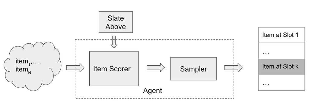
Recommendations as Contextual Bandit

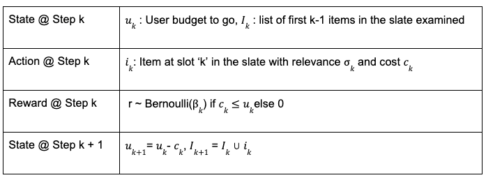
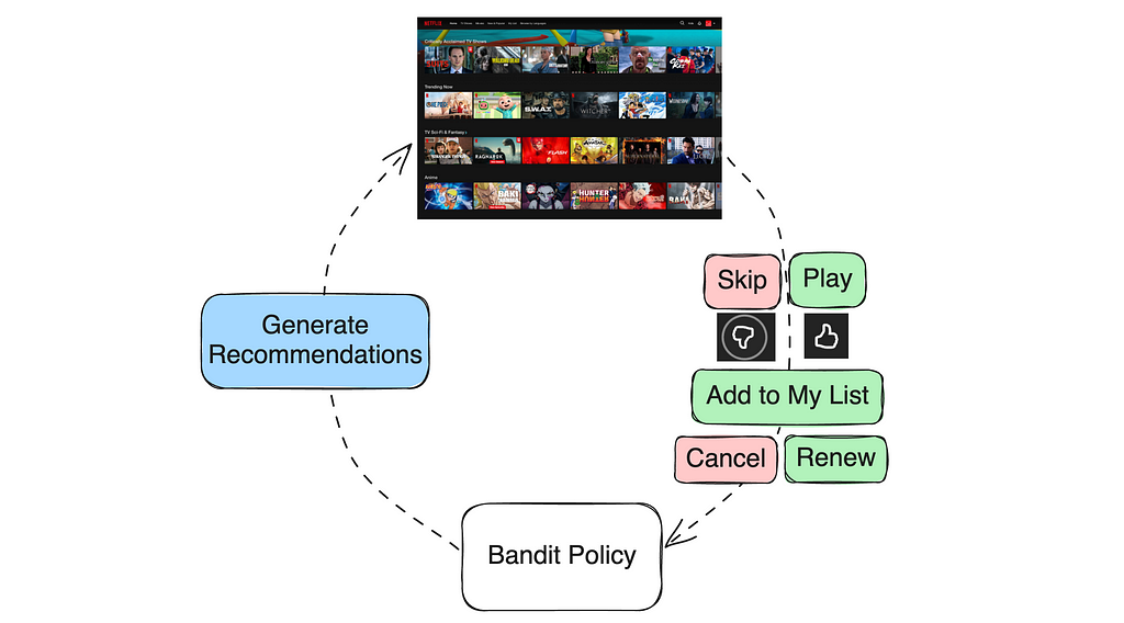
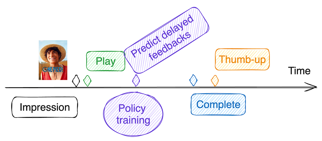
One simple way we can view recommendations is as a contextual bandit problem. When a member visits, that becomes a context for our system and it selects an action of what recommendations to show, and then the member provides various types of feedback. These feedback signals can be immediate (skips, plays, thumbs up/down, or adding items to their playlist) or delayed (completing a show or renewing their subscription). We can define reward functions to reflect the quality of the recommendations from these feedback signals and then train a contextual bandit policy on historical data to maximize the expected reward.

Improving Recommendations: Models and Objectives

There are many ways that a recommendation model can be improved. They may come from more informative input features, more data, different architectures, more parameters, and so forth. In this post, we focus on a less-discussed aspect about improving the recommender objective by defining a reward function that tries to better reflect long-term member satisfaction.

Retention as Reward?

Member retention might seem like an obvious reward for optimizing long-term satisfaction because members should stay if they’re satisfied, however it has several drawbacks:

  • Noisy: Retention can be influenced by numerous external factors, such as seasonal trends, marketing campaigns, or personal circumstances unrelated to the service.
  • Low Sensitivity: Retention is only sensitive for members on the verge of canceling their subscription, not capturing the full spectrum of member satisfaction.
  • Hard to Attribute: Members might cancel only after a series of bad recommendations.
  • Slow to Measure: We only get one signal per account per month.

Due to these challenges, optimizing for retention alone is impractical.

Proxy Rewards

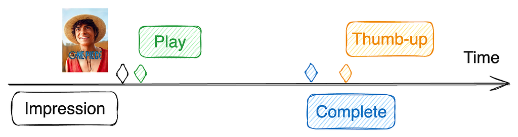
Instead, we can train our bandit policy to optimize a proxy reward function that is highly aligned with long-term member satisfaction while being sensitive to individual recommendations. The proxy reward r(user, item) is a function of user interaction with the recommended item. For example, if we recommend “One Piece” and a member plays then subsequently completes and gives it a thumbs-up, a simple proxy reward might be defined as r(user, item) = f(play, complete, thumb).

Click-through rate (CTR)

Click-through rate (CTR), or in our case play-through rate, can be viewed as a simple proxy reward where r(user, item) = 1 if the user clicks a recommendation and 0 otherwise. CTR is a common feedback signal that generally reflects user preference expectations. It is a simple yet strong baseline for many recommendation applications. In some cases, such as ads personalization where the click is the target action, CTR may even be a reasonable reward for production models. However, in most cases, over-optimizing CTR can lead to promoting clickbaity items, which may harm long-term satisfaction.

Beyond CTR

To align the proxy reward function more closely with long-term satisfaction, we need to look beyond simple interactions, consider all types of user actions, and understand their true implications on user satisfaction.

We give a few examples in the Netflix context:

  • Fast season completion ✅: Completing a season of a recommended TV show in one day is a strong sign of enjoyment and long-term satisfaction.
  • Thumbs-down after completion ❌: Completing a TV show in several weeks followed by a thumbs-down indicates low satisfaction despite significant time spent.
  • Playing a movie for just 10 minutes ❓: In this case, the user’s satisfaction is ambiguous. The brief engagement might indicate that the user decided to abandon the movie, or it could simply mean the user was interrupted and plans to finish the movie later, perhaps the next day.
  • Discovering new genres ✅ ✅: Watching more Korean or game shows after “Squid Game” suggests the user is discovering something new. This discovery was likely even more valuable since it led to a variety of engagements in a new area for a member.
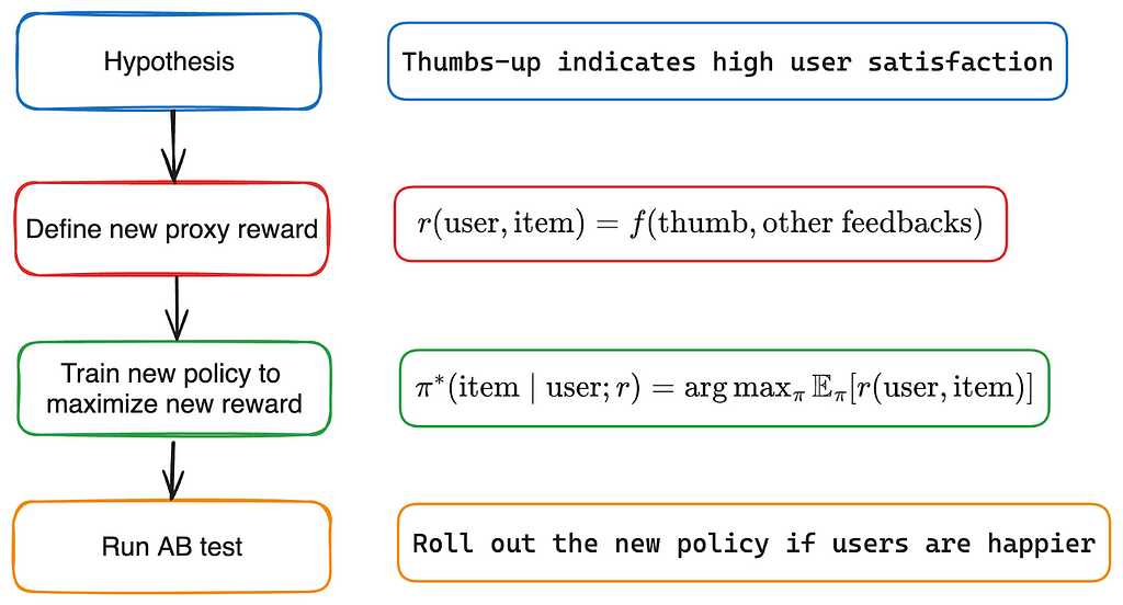
Reward Engineering

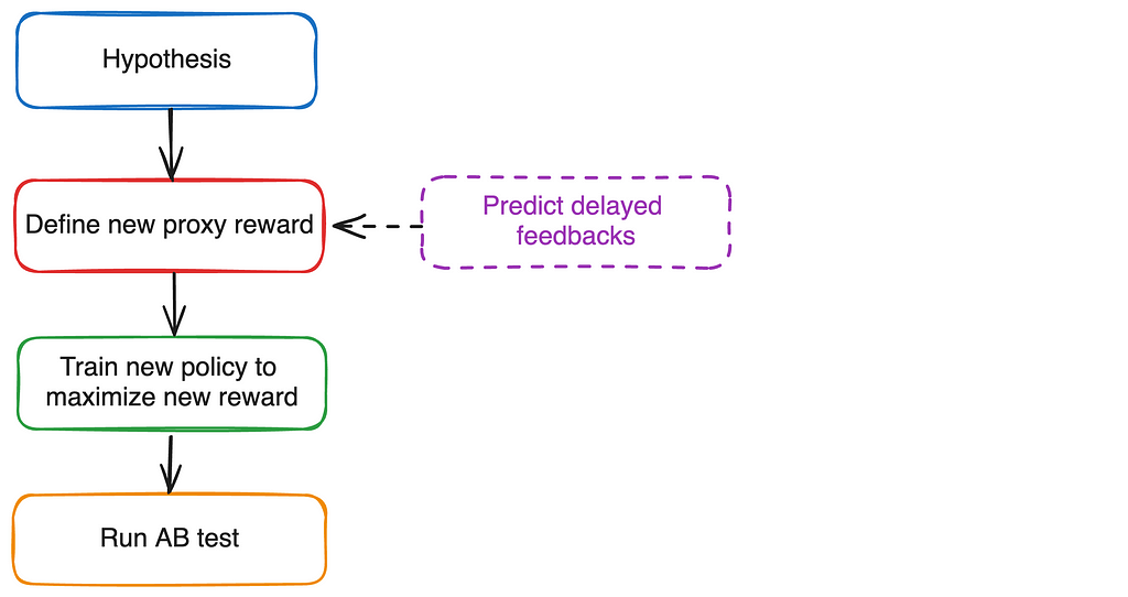
Reward engineering is the iterative process of refining the proxy reward function to align with long-term member satisfaction. It is similar to feature engineering, except that it can be derived from data that isn’t available at serving time. Reward engineering involves four stages: hypothesis formation, defining a new proxy reward, training a new bandit policy, and A/B testing. Below is a simple example.

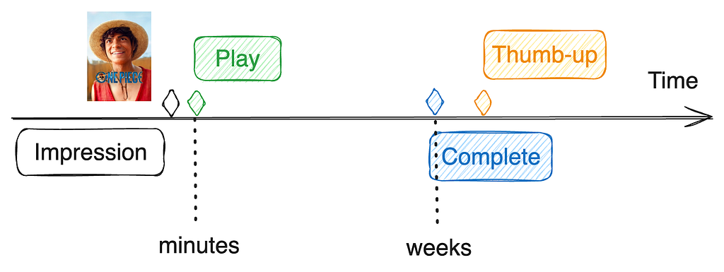
Challenge: Delayed Feedback

User feedback used in the proxy reward function is often delayed or missing. For example, a member may decide to play a recommended show for just a few minutes on the first day and take several weeks to fully complete the show. This completion feedback is therefore delayed. Additionally, some user feedback may never occur; while we may wish otherwise, not all members provide a thumbs-up or thumbs-down after completing a show, leaving us uncertain about their level of enjoyment.

We could try and wait to give a longer window to observe feedback, but how long should we wait for delayed feedback before computing the proxy rewards? If we wait too long (e.g., weeks), we miss the opportunity to update the bandit policy with the latest data. In a highly dynamic environment like Netflix, a stale bandit policy can degrade the user experience and be particularly bad at recommending newer items.

Solution: predict missing feedback

We aim to update the bandit policy shortly after making a recommendation while also defining the proxy reward function based on all user feedback, including delayed feedback. Since delayed feedback has not been observed at the time of policy training, we can predict it. This prediction occurs for each training example with delayed feedback, using already observed feedback and other relevant information up to the training time as input features. Thus, the prediction also gets better as time progresses.

The proxy reward is then calculated for each training example using both observed and predicted feedback. These training examples are used to update the bandit policy.

But aren’t we still only relying on observed feedback in the proxy reward function? Yes, because delayed feedback is predicted based on observed feedback. However, it is simpler to reason about rewards using all feedback directly. For instance, the delayed thumbs-up prediction model may be a complex neural network that takes into account all observed feedback (e.g., short-term play patterns). It’s more straightforward to define the proxy reward as a simple function of the thumbs-up feedback rather than a complex function of short-term interaction patterns. It can also be used to adjust for potential biases in how feedback is provided.

The reward engineering diagram is updated with an optional delayed feedback prediction step.

Two types of ML models

It’s worth noting that this approach employs two types of ML models:

  • Delayed Feedback Prediction Models: These models predict p(final feedback | observed feedbacks). The predictions are used to define and compute proxy rewards for bandit policy training examples. As a result, these models are used offline during the bandit policy training.
  • Bandit Policy Models: These models are used in the bandit policy π(item | user; r) to generate recommendations online and in real-time.

Challenge: Online-Offline Metric Disparity

Improved input features or neural network architectures often lead to better offline model metrics (e.g., AUC for classification models). However, when these improved models are subjected to A/B testing, we often observe flat or even negative online metrics, which can quantify long-term member satisfaction.

This online-offline metric disparity usually occurs when the proxy reward used in the recommendation policy is not fully aligned with long-term member satisfaction. In such cases, a model may achieve higher proxy rewards (offline metrics) but result in worse long-term member satisfaction (online metrics).

Nevertheless, the model improvement is genuine. One approach to resolve this is to further refine the proxy reward definition to align better with the improved model. When this tuning results in positive online metrics, the model improvement can be effectively productized. See [1] for more discussions on this challenge.

Summary and Open Questions

In this post, we provided an overview of our reward engineering efforts to align Netflix recommendations with long-term member satisfaction. While retention remains our north star, it is not easy to optimize directly. Therefore, our efforts focus on defining a proxy reward that is aligned with long-term satisfaction and sensitive to individual recommendations. Finally, we discussed the unique challenge of delayed user feedback at Netflix and proposed an approach that has proven effective for us. Refer to [2] for an earlier overview of the reward innovation efforts at Netflix.

As we continue to improve our recommendations, several open questions remain:

  • Can we learn a good proxy reward function automatically by correlating behavior with retention?
  • How long should we wait for delayed feedback before using its predicted value in policy training?
  • How can we leverage Reinforcement Learning to further align the policy with long-term satisfaction?

References

[1] Deep learning for recommender systems: A Netflix case study. AI Magazine 2021. Harald Steck, Linas Baltrunas, Ehtsham Elahi, Dawen Liang, Yves Raimond, Justin Basilico.

[2] Reward innovation for long-term member satisfaction. RecSys 2023. Gary Tang, Jiangwei Pan, Henry Wang, Justin Basilico.


Recommending for Long-Term Member Satisfaction at Netflix was originally published in Netflix TechBlog on Medium, where people are continuing the conversation by highlighting and responding to this story.

Reinforcement Learning for Budget Constrained Recommendations

Post Syndicated from Netflix Technology Blog original https://netflixtechblog.com/reinforcement-learning-for-budget-constrained-recommendations-6cbc5263a32a

by Ehtsham Elahi
with
James McInerney, Nathan Kallus, Dario Garcia Garcia and Justin Basilico

Introduction

This writeup is about using reinforcement learning to construct an optimal list of recommendations when the user has a finite time budget to make a decision from the list of recommendations. Working within the time budget introduces an extra resource constraint for the recommender system. It is similar to many other decision problems (for e.g. in economics and operations research) where the entity making the decision has to find tradeoffs in the face of finite resources and multiple (possibly conflicting) objectives. Although time is the most important and finite resource, we think that it is an often ignored aspect of recommendation problems.

In addition to relevance of the recommendations, time budget also determines whether users will accept a recommendation or abandon their search. Consider the scenario that a user comes to the Netflix homepage looking for something to watch. The Netflix homepage provides a large number of recommendations and the user has to evaluate them to choose what to play. The evaluation process may include trying to recognize the show from its box art, watching trailers, reading its synopsis or in some cases reading reviews for the show on some external website. This evaluation process incurs a cost that can be measured in units of time. Different shows will require different amounts of evaluation time. If it’s a popular show like Stranger Things then the user may already be aware of it and may incur very little cost before choosing to play it. Given the limited time budget, the recommendation model should construct a slate of recommendations by considering both the relevance of the items to the user and their evaluation cost. Balancing both of these aspects can be difficult as a highly relevant item may have a much higher evaluation cost and it may not fit within the user’s time budget. Having a successful slate therefore depends on the user’s time budget, relevance of each item as well as their evaluation cost. The goal for the recommendation algorithm therefore is to construct slates that have a higher chance of engagement from the user with a finite time budget. It is important to point out that the user’s time budget, like their preferences, may not be directly observable and the recommender system may have to learn that in addition to the user’s latent preferences.

A typical slate recommender system

We are interested in settings where the user is presented with a slate of recommendations. Many recommender systems rely on a bandit style approach to slate construction. A bandit recommender system constructing a slate of K items may look like the following:

A bandit style recommender system for slate construction

To insert an element at slot k in the slate, the item scorer scores all of the available N items and may make use of the slate constructed so far (slate above) as additional context. The scores are then passed through a sampler (e.g. Epsilon-Greedy) to select an item from the available items. The item scorer and the sampling step are the main components of the recommender system.

Problem formulation

Let’s make the problem of budget constrained recommendations more concrete by considering the following (simplified) setting. The recommender system presents a one dimensional slate (a list) of K items and the user examines the slate sequentially from top to bottom.

A user with a fixed time budget evaluating a slate of recommendations with K items. Item 2 gets the click/response from the user. The item shaded in red falls outside of the user’s time budget.

The user has a time budget which is some positive real valued number. Let’s assume that each item has two features, relevance (a scalar, higher value of relevance means that the item is more relevant) and cost (measured in a unit of time). Evaluating each recommendation consumes from the user’s time budget and the user can no longer browse the slate once the time budget has exhausted. For each item examined, the user makes a probabilistic decision to consume the recommendation by flipping a coin with probability of success proportional to the relevance of the video. Since we want to model the user’s probability of consumption using the relevance feature, it is helpful to think of relevance as a probability directly (between 0 and 1). Clearly the probability to choose something from the slate of recommendations is dependent not only on the relevance of the items but also on the number of items the user is able to examine. A recommendation system trying to maximize the user’s engagement with the slate needs to pack in as many relevant items as possible within the user budget, by making a trade-off between relevance and cost.

Connection with the 0/1 Knapsack problem

Let’s look at it from another perspective. Consider the following definitions for the slate recommendation problem described above

Clearly the abandonment probability is small if the items are highly relevant (high relevance) or the list is long (since the abandonment probability is a product of probabilities). The abandonment option is sometimes referred to as the null choice/arm in bandit literature.

This problem has clear connections with the 0/1 Knapsack problem in theoretical computer science. The goal is to find the subset of items with the highest total utility such that the total cost of the subset is not greater than the user budget. If β_i and c_i are the utility and cost of the i-th item and u is the user budget, then the budget constrained recommendations can be formulated as

0/1 Knapsack formulation for Budget constrained recommendations

There is an additional requirement that optimal subset S be sorted in descending order according to the relevance of items in the subset.

The 0/1 Knapsack problem is a well studied problem and is known to be NP-Complete. There are many approximate solutions to the 0/1 Knapsack problem. In this writeup, we propose to model the budget constrained recommendation problem as a Markov Decision process and use algorithms from reinforcement learning (RL) to find a solution. It will become clear that the RL based solution to budget constrained recommendation problems fits well within the recommender system architecture for slate construction. To begin, we first model the budget constrained recommendation problem as a Markov Decision Process.

Budget constrained recommendations as a Markov Decision Process

In a Markov decision process, the key component is the state evolution of the environment as a function of the current state and the action taken by the agent. In the MDP formulation of this problem, the agent is the recommender system and the environment is the user interacting with the recommender system. The agent constructs a slate of K items by repeatedly selecting actions it deems appropriate at each slot in the slate. The state of the environment/user is characterized by the available time budget and the items examined in the slate at a particular step in the slate browsing process. Specifically, the following table defines the Markov Decision Process for the budget constrained recommendation problem,

Markov Decision Process for Budget constrained recommendations

In real world recommender systems, the user budget may not be observable. This problem can be solved by computing an estimate of the user budget from historical data (e.g. how long the user scrolled before abandoning in the historical data logs). In this writeup, we assume that the recommender system/agent has access to the user budget for sake of simplicity.

The slate generation task above is an episodic task i-e the recommender agent is tasked with choosing K items in the slate. The user provides feedback by choosing one or zero items from the slate. This can be viewed as a binary reward r per item in the slate. Let π be the recommender policy generating the slate and γ be the reward discount factor, we can then define the discounted return for each state, action pair as,

State, Action Value function estimation

The reinforcement learning algorithm we employ is based on estimating this return using a model. Specifically, we use Temporal Difference learning TD(0) to estimate the value function. Temporal difference learning uses Bellman’s equation to define the value function of current state and action in terms of value function of future state and action.

Bellman’s equation for state, action value function

Based on this Bellman’s equation, a squared loss for TD-Learning is,

Loss Function for TD(0) Learning

The loss function can be minimized using semi-gradient based methods. Once we have a model for q, we can use that as the item scorer in the above slate recommender system architecture. If the discount factor γ =0, the return for each (state, action) pair is simply the immediate user feedback r. Therefore q with γ = 0 corresponds to an item scorer for a contextual bandit agent whereas for γ > 0, the recommender corresponds to a (value function based) RL agent. Therefore simply using the model for the value function as the item scorer in the above system architecture makes it very easy to use an RL based solution.

Budget constrained Recommendation Simulation

As in other applications of RL, we find simulations to be a helpful tool for studying this problem. Below we describe the generative process for the simulation data,

Generative model for simulated data

Note that, instead of sampling the per-item Bernoulli, we can alternatively sample once from a categorical distribution with relative relevances for items and a fixed weight for the null arm. The above generative process for simulated data depends on many hyper-parameters (loc, scale etc.). Each setting of these hyper-parameters results in a different simulated dataset and it’s easy to realize many simulated datasets in parallel. For the experiments below, we fix the hyper-parameters for the cost and relevance distributions and sweep over the initial user budget distribution’s location parameter. The attached notebook contains the exact settings of the hyper-parameters used for the simulations.

Metric

A slate recommendation algorithm generates slates and then the user model is used to predict the success/failure of each slate. Given the simulation data, we can train various recommendation algorithms and compare their performance using a simple metric as the average number of successes of the generated slates (referred to as play-rate below). In addition to play-rate, we look at the effective-slate-size as well, which we define to be the number of items in the slate that fit the user’s time budget. As mentioned earlier, one of the ways play-rate can be improved is by constructing larger effective slates (with relevant items of-course) so looking at this metric helps understand the mechanism of the recommendation algorithms.

On-policy learning results

Given the flexibility of working in the simulation setting, we can learn to construct optimal slates in an on-policy manner. For this, we start with some initial random model for the value function, generate slates from it, get user feedback (using the user model) and then update the value function model using the feedback and keep repeating this loop until the value function model converges. This is known as the SARSA algorithm.

The following set of results show how the learned recommender policies behave in terms of metric of success, play-rate for different settings of the user budget distributions’s location parameter and the discount factor. In addition to the play rate, we also show the effective slate size, average number of items that fit within the user budget. While the play rate changes are statistically insignificant (the shaded areas are the 95% confidence intervals estimated using bootstrapping simulations 100 times), we see a clear trend in the increase in the effective slate size (γ > 0) compared to the contextual bandit (γ= 0)

Play-Rate and Effective slate sizes for different User Budget distributions. The user budget distribution’s location is on the same scale of the item cost and we are looking for changes in the metrics as we make changes to the user budget distribution

We can actually get a more statistically sensitive result by comparing the result of the contextual bandit with an RL model for each simulation setting (similar to a paired comparison in paired t-test). Below we show the change in play rate (delta play rate) between any RL model (shown with γ = 0.8 below as an example) and a contextual bandit (γ = 0). We compare the change in this metric for different user budget distributions. By performing this paired comparison, we see a statistically significant lift in play rate for small to medium budget user budget ranges. This makes intuitive sense as we would expect both approaches to work equally well when the user budget is too large (therefore the item’s cost is irrelevant) and the RL algorithm only outperforms the contextual bandit when the user budget is limited and finding the trade-off between relevance and cost is important. The increase in the effective slate size is even more dramatic. This result clearly shows that the RL agent is performing better by minimizing the abandonment probability by packing more items within the user budget.

Paired comparison between RL and Contextual bandit. For limited user budget settings, we see statistically significant lift in play rate for the RL algorithm.

Off-policy learning results

So far the results have shown that in the budget constrained setting, reinforcement learning outperforms contextual bandit. These results have been for the on-policy learning setting which is very easy to simulate but difficult to execute in realistic recommender settings. In a realistic recommender, we have data generated by a different policy (called a behavior policy) and we want to learn a new and better policy from this data (called the target policy). This is called the off-policy setting. Q-Learning is one well known technique that allows us to learn optimal value function in an off-policy setting. The loss function for Q-Learning is very similar to the TD(0) loss except that it uses Bellman’s optimality equation instead

Loss function for Q-Learning

This loss can again be minimized using semi-gradient techniques. We estimate the optimal value function using Q-Learning and compare its performance with the optimal policy learned using the on-policy SARSA setup. For this, we generate slates using Q-Learning based optimal value function model and compare the play-rate with the slates generated using the optimal policy learned with SARSA. Below is result of the paired comparison between SARSA and Q-Learning,

Paired comparison between Q-Learning and SARSA. Play rates are similar between the two approaches but effective slate sizes are very different.

In this result, the change in the play-rate between on-policy and off-policy models is close to zero (see the error bars crossing the zero-axis). This is a favorable result as this shows that Q-Learning results in similar performance as the on-policy algorithm. However, the effective slate size is quite different between Q-Learning and SARSA. Q-Learning seems to be generating very large effective slate sizes without much difference in the play rate. This is an intriguing result and needs a little more investigation to fully uncover. We hope to spend more time understanding this result in future.

Conclusion:

To conclude, in this writeup we presented the budget constrained recommendation problem and showed that in order to generate slates with higher chances of success, a recommender system has to balance both the relevance and cost of items so that more of the slate fits within the user’s time budget. We showed that the problem of budget constrained recommendation can be modeled as a Markov Decision Process and we can find a solution to optimal slate construction under budget constraints using reinforcement learning based methods. We showed that the RL outperforms contextual bandits in this problem setting. Moreover, we compared the performance of On-policy and Off-policy approaches and found the results to be comparable in terms of metrics of success.

Code

Github repo


Reinforcement Learning for Budget Constrained Recommendations was originally published in Netflix TechBlog on Medium, where people are continuing the conversation by highlighting and responding to this story.