Over the first weekend in November, members of the global Code Club community came together for two inspiring days of learning, creativity and connection. The annual event celebrates the people who make Code Clubs happen, allowing them to share ideas, explore new tools, and connect with others who help young people learn to code.
Exploring new technologies and inclusive teaching
Saturday began with hands-on sessions that brought creativity and technology together, exploring large language models and prompt engineering in Collaborating with LLMs and being a prompt boss. There was a lot of laughter from attendees about how large language models can produce confident but incorrect answers if given vague prompts, but many left inspired to experiment with new technologies in their own clubs.
“First time there and it was amazing. Met loads of great people and the amazing code club crew. I learnt loads of new skills around AI and Arduino.” – An attendee
Collaboration that counts brought mentors together to discuss common challenges like volunteer retention, limited resources, and communication barriers. A crowd favourite was a shared volunteer toolkit, as well as event checklists and safeguarding resources.
“What I enjoyed most about the Clubs Conference was the opportunity to meet other facilitators and hear their stories — their successes and challenges. These conversations validated the volunteer work I do and reminded me of the impact of our clubs.” – An attendee
From the theatre sessions, you can watch Inclusive learning – Supporting Deaf learners in clubs which was both moving and insightful. We learnt that visual demonstrations, colour cues, and repetition were key to supporting Deaf learners. One memorable quote captured the spirit of the session:
“The children couldn’t speak to us. The children — we couldn’t hear their voices but by the eighth week we were able to hear their voices from what they built on the screen and it was echoing all around the classroom.” – Chidi Duru
The weekend’s talks showcased the reach of Code Club worldwide, with volunteers sharing their experiences of collaboration, sustainability, and creativity.
WatchLessons from resourceful Code Clubs in India, which highlighted the ingenuity of young learners in under-resourced settings, while Hands-on with the Raspberry Pi Pico showcased low-cost, high-impact projects from Kenya and South Africa.
Speakers showed how community clubs adapt to local needs with unplugged activities and coding games inspired by cricket and kabaddi, empowering young people to solve real problems and celebrate curiosity through play. Excitingly, these new resources will be launching early next year; keep an eye on our activities page to be among the first to try them out!
In the session Code Club Projects Unplugged, facilitators shared the idea of “hiding the vegetables” — hiding the learning inside the fun. Whether through a collaborative Scratch game, a micro:bit prop on stage, or a Pico gadget solving a real problem, this approach helps young people learn through play. They remember the joy, and the skills come naturally.
Learning beyond the screen
Teaching tech away from the computer screen shared a fun unplugged cybersecurity activity, The Chicken Shop, where learners role-play social engineering scenarios. Its success came from clear printed instructions, movement, humour, and strong debriefing.
Learning coding outside the box explored how to engage young people with diverse learning styles while the Arduino crash course gave attendees a taste of physical computing and C++ programming in action. Workshops on AI, sustainability, and youth empowerment with Raspberry Pi computers and Unlocking Code Club resources helped club leaders discover practical ways to inspire problem-solving and make use of all the support available through Code Club.
The message from the sessions was clear: young people learn best when technology is human and hands-on.
Showcasing creativity with Coolest Projects
Coolest Projects – get involved!championed creativity over competition. Any young person under 18 can submit their project, including unfinished ideas. In-person and online showcases celebrate progress, imagination, and teamwork.
Speaking on the closing panel, Code Club leader Rachael Coultart talked about the importance of Coolest Projects as a rare platform for children to talk about their learning. She spoke about the experience of one particular child, explaining that it had made a powerful impression on her, saying:
“It had such a huge impact. I felt so proud of her and what she’d achieved. Afterwards, her parents told me that they felt it was the first time she had really been seen.”
What the community is taking forward
The community is united in its commitment to making Code Clubs inclusive, creative, and sustainable.
Context matters — projects that reflect local interests and challenges motivate young people to learn
Accessibility is central: visual cues, repetition, interpreters, and inclusive resources support every learner
Structure builds confidence; start with simple, guided activities before open-ended exploration
Volunteers are vital; shared toolkits, checklists, and training help them deliver engaging sessions
Celebration and affordability matter too: regular showcases and tools like the micro:bit, Pico, and Crumble keep computing fun, hands-on, and accessible for all
“Thank you. Clubs Conference is a highlight of my year.” – An attendee
Stay connected
If you want to stay up to date with the latest news, events and opportunities from Code Club, sign up for our newsletter and be part of the growing global community.
Operate systems reliably in production with minimal overhead, at Netflix scale.
Metaflow works with many battle-hardened tooling to address the second point — among them Maestro, our newly open-sourced workflow orchestrator that powers nearly every ML and AI system at Netflix and serves as a backbone for Metaflow itself.
In this post, we focus on the first point and introduce a new Metaflow functionality, Spin, that helps users accelerate their iterative development process. By the end, you’ll have a solid understanding of Spin’s capabilities and learn how to try it out yourself with Metaflow 2.19.
Iterative development in ML and AI workflows
Developing a Metaflow flow with cards in VSCode
To understand our approach to improving the ML and AI development experience, it helps to consider how these workflows differ from traditional software engineering.
ML and AI development revolves not just around code but also around data and models, which are large, mutable, and computationally expensive to process. Iteration cycles can involve long-running data transformations, model training, and stochastic processes that yield slightly different results from run to run. These characteristics make fast, stateful iteration a critical part of productive development.
This is where notebooks — such as Jupyter, Observable, or Marimo — shine. Their ability to preserve state in memory allows developers to load a dataset once and iteratively explore, transform, and visualize it without reloading or recomputing from scratch. This persistent, interactive environment turns what would otherwise be a slow, rigid loop into a fluid, exploratory workflow — perfectly suited to the needs of ML and AI practitioners.
Because ML and AI development is computationally intensive, stochastic, and data- and model-centric, tools that optimize iteration speed must treat state management as a first-class design concern. Any system aiming to improve the development experience in this domain must therefore enable quick, incremental experimentation without losing continuity between iterations.
New: rapid, iterative development with spin
At first glance, Metaflow code looks like a workflow — similar to Airflow — but there’s another way to look at it: each Metaflow @step serves as a checkpoint boundary. At the end of every step, Metaflow automatically persists all instance variables as artifacts, allowing the execution to resume seamlessly from that point onward. The below animation shows this behavior in action:
Using resume in Metaflow
In a sense, we can consider a @step similar to a notebook cell: it is the smallest unit of execution that updates state upon completion. It does have a few differences that address the issues with notebook cells:
The execution order is explicit and deterministic: no surprises due to out-of-order cell execution;
The state is not hidden: state is explicitly stored as self. variables as shared state, which can be discovered and inspected;
The state is versioned and persisted making results more reproducible.
While Metaflow’s resume feature can approximate the incremental and iterative development approach of notebooks, it restarts execution from the selected step onward, introducing more latency between iterations. In contrast, a notebook allows near-instant feedback by letting users tweak and rerun individual cells while seamlessly reusing data from earlier cells held in memory.
The new spin command in Metaflow 2.19 addresses this gap. Similar to executing a single notebook cell, it quickly executes a single Metaflow @step — with all the state carried over from the parent step. As a result, users can develop and debug Metaflow steps as easily as a cell in a notebook.
The effect becomes clear when considering the three complementary execution modes — run, resume, and spin — side by side, mapping them to the corresponding notebook behavior:
Run, Resume and Spin “modes”
Another major difference isn’t just what gets executed, but what gets recorded. Both run and resume create a full, versioned run with complete metadata and artifacts, while spin skips tracking altogether. It’s built for fast, throw-away iterations during development.
The one-minute clip below illustrates a typical iterative development workflow that alternates between run and spin. In this example, we are building a flow that reads a dataset from a Parquet file and trains a separate model for each product category, focusing on computer-related categories.
As shown in the video, we start by creating a flow from scratch and running a minimal version of it to persist test artifacts — in this case, a Parquet dataset. From there, we can use spin to iterate on one step at a time, incrementally building out the flow, for example, by adding the parallel training steps demonstrated in the clip.
Once the flow has been iterated on locally, it can be seamlessly deployed to production orchestrators like Maestro or Argo, and scaled up on compute platforms such as AWS Batch, Titus, Kubernetes and more. Thus, the experience is as smooth as developing in a notebook, but the outcome is a production-ready, scalable workflow, implemented as an idiomatic Python project!
Spin up smooth development in VSCode/Cursor
Instead of typing run and spin manually in the terminal, we can bind them to keyboard shortcuts. For example, the simple metaflow-dev VS Code extension (works with Cursor as well) maps Ctrl+Opt+R to run and Ctrl+Opt+S to spin. Just hack away, hit Ctrl+Opt+S, and the extension will save your file and spin the step you are currently editing.
One area where spin truly shines is in creating mini-dashboards and reports with Metaflow Cards. Visualization is another strong point of notebooks but the combination of spin and cards makes Metaflow a very compelling alternative for developing real-time and post-execution visualizations. Developing cards is inherently iterative and visual (much like building web pages) where you want to tweak code and see the results instantly. This workflow is readily available with the combination of VSCode/Cursor, which includes a built-in web-view, the local card viewer, and spin.
To see the trio of tools — along with the VS Code extension — in action, in this short clip we add observability to the train step that we built in the earlier example:
A major benefit of Metaflow Cards is that we don’t need to deploy any extra services, data streams, and databases for observability. Just develop visual outputs as above, deploy the flow, and wehave a complete system in production with reporting and visualizations included.
Spin to the next level: injecting inputs, inspecting outputs
Spin does more than just run code — it also lets us take full control of a spun @step’s inputs and outputs, enabling a range of advanced patterns.
In contrast to notebooks, we can spin any arbitrary @step in a flow using state from any past run, making it easy to test functions with different inputs. For example, if we have multiple models produced by separate runs, we could spin an inference step, supplying a different model run each time.
We can also override artifact values or inject arbitrary Python objects — similar to a notebook cell — for spin. Simply specify a Python module with an ARTIFACTS dictionary:
ARTIFACTS = {
  "model": "kmeans",
  "k": 15
}
and point spin at the module:
spin train --artifacts-module artifacts.py
By default spin doesn’t persist artifacts, but we can easily change this by adding –persist. Even in this case, artifacts are not persisted in the usual Metaflow datastore but to a directory-specific location which you can easily clean up after testing. We can access the results with the Client API as usual — just specify the directory you want to inspect with inspect_spin:
Being able to inspect and modify a step’s inputs and outputs on the fly unlocks a powerful use case: unit testing individual steps. We can use spin programmatically through the Runner API and assert the results:
from metaflow import Runner

with Runner("flow.py").spin("train", persist=True) as spin:
  assert spin.task["model"].data == "kmeans"
Making AI agents spin
In addition to speeding up development for humans, spin turns out to be surprisingly handy for coding agents too. There are two major advantages to teaching AI how to spin:
It accelerates the development loop. Agents don’t naturally understand what’s slow, or why speed matters, so they need to be nudged to favor faster tools over slower ones.
It helps surface errors faster and contextualizes them to a specific piece of code, increasing the chance that the agent is able to fix errors by itself.
Metaflow users are already using Claude Code; spin makes this even easier. In the example below, we added the following section in a CLAUDE.md file:
## Developing Metaflow code
Follow this incremental development workflow that ensures quick iterations
and correct results. You must create a flow incrementally, step by step
following this process:
1. Create a flow skeleton with empty `@step`s.
2. Add a data loading step.
3. `run` the flow.
4. Populate the next step and use `spin` to test it with the correct inputs.
5. `run` the flow to record outputs from the new step.
5. Iterate on (4–5) until all steps have been implemented and work correctly.
6. `run` the whole flow to ensure final correctness.

To test a flow, run the flow as follows
```
python flow.py - environment=pypi run
```

Do this once before running `spin`.
As you are building the flow, you `spin` to test steps quickly.
For instance
```
python flow.py - environment=pypi spin train
```
Just based on these quick instructions, the agent is able to use spin effectively. Take a look at the following inspirational example that one-shots Claude to create a flow, along the lines of our earlier examples, which trains a classifier to predict product categories:
In the video, we can see Claude using spin around the 45-second mark to test a preprocess step. The step initially fails due to a classic data science pitfall: during testing, Claude samples only a small subset of data, causing some classes to be underrepresented. The first spin surfaces the issue, which Claude then fixes by switching to stratified sampling — and finally does another spin to confirm the fix, before proceeding to complete the task.
The inner loop of end-to-end ML/AI
To circle back to where we started, our motivation for adding spin — and for creating Metaflow in the first place — is to accelerate development cycles so we can deliver more joy to our subscribers, faster. Ultimately, we believe there’s no single magic feature that makes this possible. It takes all parts of an ML/AI platform working together coherently — spin included.
From this perspective, it’s useful to place spin in the context of other Metaflow features. It’s designed for the innermost loop of model and business-logic development, with the added benefit of supporting unit testing during deployment, as shown in the overall blueprint of the Metaflow toolchain below.
Metaflow tool-chain
In this diagram, the solid blue boxes represent different Metaflow commands, while the blue text denotes decorators and other features. In particular, note the Shared Functionality box — another key focus area for us over the past year — which includes configuration management and custom decorators. These capabilities let domain-specific teams and platform providers tailor Metaflow to their own use cases. Following our ethos of composability, all of these features integrate seamlessly with spin as well.
Another key design philosophy of Metaflow is to let projects start small and simple, adding complexity only when it becomes necessary. So don’t be overwhelmed by the diagram above. To get started, install Metaflow easily with
pip install metaflow
and take your first baby @steps for a spin! Check out the docs and for questions, support, and feedback, join the friendly Metaflow Community Slack.
Current artificial intelligence (AI) methods, especially machine learning (ML), rely heavily on data. To complement our work on AI literacy, we have been investigating what data science teaching resources and education research are currently available. Our goal is to work out what data science concepts should be taught in a data science curriculum for schools.
Read on to find out what resources and materials we have reviewed, and what concept themes we have identified.
What is data science? Why is teaching it important?
Data science is an interdisciplinary science of learning from large datasets, aided by modern computational tools and methods (Ow‑Yeong et al., 2023). We see data science skills as fundamental for using, creating, and thinking critically about:
Insights from data, generally
Data-driven computational tools and methods (such as machine learning) and their outputs and predictions, specifically
To navigate a world where decision making in many areas is influenced by data-driven insights and predictions, young people need to be taught about data science. Data science skills empower young people to become critical thinkers, discerning consumers, adaptable professionals, and informed citizens.
In some countries, such as India and Israel, data science education is an established school subject. It is taught as part of the curriculum in at least one of the primary, secondary, or post-16 age phases. Meanwhile in other countries, for example Canada, Germany, and Poland, data science is a very new school subject, or there are still only recommendations to develop it into a school subject.
While we are currently considering what a comprehensive data science curriculum should include, we already offer several resources to support you with your teaching about data science and data-driven technologies. You can find a list of these resources at the end of this blog. Now, however, I’ll give you an overview of our recent work to identify concepts for a data science curriculum that fits with our approach to AI literacy.
Data science education: What should we teach?
To answer the question ‘What should we teach about data science to learners aged 5 to 19?’, we undertook a grey literature review of data science teaching materials. A grey literature review is structured like an academic literature review and conducted with the same rigour. The difference is that a grey literature review also considers publications that have not been peer-reviewed, including reports, white papers, curriculum materials, and similar resources.
To orient our work, we combined four frameworks for data science and AI/ML education:
With these combined frameworks as our map, we reviewed 79 data science learning resources. The resources varied:
In quality in terms of clarity and teaching approach
In their focus, e.g. on maths, coding, or a specific field such as biology
In their perspective on data science, with some prioritising theory and others real-world applications
From among the 79 resources, we chose 9 that included clear learning outcomes, and that together covered a wide field of concepts. We examined these 9 in detail to extract 181 explicit and implicit data science concepts. Next, we grouped the concepts into themes, and finally we refined these themes by comparing them against the four frameworks listed above.
The themes we have identified for a data science curriculum are:
Fundamentals of data literacy: Key terms and definitions
Understanding bias in data
Ethical responsibility in data use
Data creation, curation, and transformation
Analysis and modelling: Maths and statistics fundamentals
ML principles
Deploying and maintaining ML applications
Software tools and programming
Data visualisation
Presenting findings effectively
This set of themes both fits with the frameworks by Olari and Romeike and Data Science 4 Everyone, and expands them by covering ML principles and programming approaches and calling out data bias and ethics.
What’s next for this work?
Through our grey literature review on data science education, we’ve:
Pinpointed a large set of candidate concepts that could be taught within a data science curriculum
Created a set of clear themes to structure our work going forward
Our next step is to shape these candidate concepts into a progression framework to describe their relationships and establish which concepts could be taught at each age or phase of schooling.
The literature review also gave us an overview of the pedagogical approaches and tools used for teaching data science concepts. These findings will become useful once we start designing learning activities.
You’ll hear more about how this work is going here on our blog and on our social channels. In the meantime, comment below to let us know what you think about the themes, or to tell us what you’d like to see in a data science curriculum for the learners you work with.
The report lists the data-related units within The Computing Curriculum materials, which we no longer update but continue to offer as free downloads. Updated classroom materials are available as part of the Computing materials we created for Oak National Academy in the UK for ages 5–11 and ages 12–19.
The Ada Computer Science platform offers learning materials on data and information, and on AI and ML, for ages 14–19.
You might also be interested in exploring the Experience AI programme, which offers everything teachers need to help students develop a foundational understanding of data-driven AI technologies, their social and ethical implications, and the role that AI can play in their lives.
Teacher training and development resources
Our free online course ‘Teach teens computing: Machine learning and AI‘ helps teachers understand and explain the types of problems that ML can help to solve, discuss how AI is changing the world, and think about the ethics of collecting data to train a ML model.
Teaching young people to understand data-driven AI technologies means teaching them thinking skills that are different to those needed to understand rule-based computer systems. You can read about these Computational Thinking 2.0 skills in our Quick Read PDF.
We recently upgraded the Maestro engine to go beyond scalability and improved its performance by 100X! The overall overhead is reduced from seconds to milliseconds. We have updated the Maestro open source project with this improvement! Please visit the Maestro GitHub repository to get started. If you find it useful, please give us a star.
Introduction
In our previous blog post, we introduced Maestro as a horizontally scalable workflow orchestrator designed to manage large-scale Data/ML workflows at Netflix. Over the past two and a half years, Maestro has achieved its design goal and successfully supported massive workflows with hundreds of thousands of jobs, managing millions of executions daily. As the adoption of Maestro increases at Netflix, new use cases have emerged, driven by Netflix’s evolving business needs, such as Live, Ads, and Games. To meet these needs, some of the workflows are now scheduled on a sub-hourly basis. Additionally, Maestro is increasingly being used for low-latency use cases, such as ad hoc queries, beyond traditional daily or hourly scheduled ETL data pipeline use cases.
While Maestro excels in orchestrating various heterogeneous workflows and managing user end-to-end development experiences, users have experienced noticeable speedbumps (i.e. ten seconds overhead) from the Maestro engine during workflow executions and development, affecting overall efficiency and productivity. Although being fully scalable to support Netflix-scale use cases, the processing overhead from Maestro internal engine state transitions and lifecycle activities have become a bottleneck, particularly during development cycles. Users have expressed the need for a high performance workflow engine to support iterative development use cases.
To visualize our end users’ needs for the workflow orchestrator, we create a 5-layer structure graph shown below. Before the change, Maestro reached level 4 but faced challenges to satisfy the user’s needs in level 5. With the new engine design, Maestro is able to power the users to work with their highest capacity and spark joy for end users during their development over the Maestro.
Figure 1. A 5-layer structure showing needs for the workflow orchestrator.
In this blog post, we will share our new engine details, explain our design trade-off decisions, and share learnings from this redesign work.
Architectural Evolution of Maestro
Before the change
To understand the improvements, we will first revisit the original architecture of Maestro to understand why the overhead is high. The system was divided into three main layers, as illustrated in the diagram below. In the sections that follow we will explain each layer and the role it played in our performance optimization.
Figure 2. The architecture diagram before the evolution.
Maestro API and Step Runtime Layer
This layer offers seamless integrations with other Netflix services (e.g., compute engines like Spark and Trino). Using Maestro, thousands of practitioners build production workflows using a paved path to access platform services . They can focus primarily on their business logic while relying on Maestro to manage the lifecycle of jobs and workflows plus the integration with data platform services and required integrations such as for authentication, monitoring and alerting. This layer functioned efficiently without introducing significant overhead.
Maestro Engine Layer
The Maestro engine serves several crucial functions:
Managing the lifecycle of workflows, their steps and maintaining their state machines
Supporting all user actions (e.g., start, restart, stop, pause) on workflow and step entities
Translating complex Maestro workflow graphs into parallel flows, where each flow is an array of sequentially chained flow tasks, translating every step into a flow task, and then executing transformed flows using the internal flow engine
Acting as a middle layer to maintain isolation between the Maestro step runtime layer and the underlying flow engine layer
Implementing required data access patterns and writing Maestro data into the database
In terms of speed, this layer had acceptable overhead but faced edge cases (e.g. a step might be concurrently executed by two workers at the same time, causing race conditions) due to lacking a strong guarantee from the internal flow engine and the external distributed job queue.
Maestro Internal Flow Engine Layer
The Maestro internal flow engine performed 2 primary functions:
Calling task’s execution functions at a given interval.
Starting the next tasks in an array of sequential task flows (not a graph), if applicable.
This foundational layer was based on Netflix OSS Conductor 2.x (deprecated since Apr 2021), which requires a dedicated set of separate database tables and distributed job queues.
The existing implementation of this layer introduces an impactful overhead (e.g. a few seconds to tens of seconds overall delays). The lack of strong guarantees (e.g. exactly once publishing) from this layer leads to race conditions which cause stuck jobs or lost executions.
Options to consider
We have evaluated three options to address those existing issues:
Option 1: Implement an internal flow engine optimized for Maestro specific use cases
Option 2: Upgrade Conductor library to 4.0, which addresses the overheads and offers other improvements and enhancements compared with Conductor 2.X.
Option 3: Use Temporal as the internal flow engine
One aspect that influenced our assessment of option two is that Conductor 2 provided a final callback capability in the state machine that was contributed specifically for Maestro’s use case to ensure database synchronization between the Conductor and Maestro engine states. It would require porting this functionality to Conductor 4 though it had been dropped given no other Conductor use cases besides Maestro relied on this. By rewriting the flow engine it would allow removal of several complex internal databases and database synchronization requirements which was attractive for simplifying operational reliability. Given Maestro did not need the full set of state engine features offered by Conductor, this motivated us to consider a flow engine rewrite as a higher priority.
The decision for Temporal was more straightforward. Temporal is optimized towards facilitating inter-process orchestration and would involve calling an external service to interact with the Temporal flow engine. Given Maestro is operating greater than a million tasks per day, many of which are long running, we felt it was an unnecessary source of risk to couple the DAG engine execution with an external service call. If our requirements went beyond lightweight state transition management we might reconsider because Temporal is a very robust control plane orchestration system, but for our needs it introduced complexity and potential reliability weak spots when there was no direct need for the advanced feature set that it offered.
After considering Option 2 and Option 3, we developed more conviction that Maestro’s architecture could be greatly simplified by not using a full DAG evaluation engine and having to maintain the state machine for two systems (Maestro and Conductor/Temporal). Therefore, we have decided to go with Option 1.
After the change
To address these issues, we completely rewrote the Maestro internal flow engine layer to satisfy Maestro’s specific needs and optimize its performance. This new flow engine is lightweight with minimal dependencies, focusing on excelling in the two primary functions mentioned above. We also replaced existing distributed job queues with internal ones to provide a strong guarantee.
The new engine is highly performant, efficient, scalable, and fault-tolerant. It is the foundation for all upper components of Maestro and provides the following guarantees to avoid race conditions:
A single step should only be executed by a single worker at any given time
Step state should never be rolled back
Steps should always eventually run to a terminal state
The internal flow state should be eventually consistent with the Maestro workflow state
External API and user actions should not cause race conditions on the workflow execution
Here is the new architecture diagram after the change, which is much simpler with less dependencies:
Figure 3. The architecture diagram after the evolution.
New Flow Engine Optimization
The new flow engine significantly boosts speed by maintaining state in memory. It ensures consistency by using Maestro engine’s database as the source of truth for workflow and step states. During bootstrapping, the flow engine rebuilds its in-memory state from the database, improving performance and simplifying the overall architecture. This is in contrast to the previous design in which multiple databases had to be reconciled against one another (Conductor’s tables and Maestro’s tables) or else suffer race conditions and rare orphaned job status.
The flow engine operates on in-memory flow states, resembling a write through caching pattern. Updates to workflow or step state in the database also update the in-memory flow state. If in-memory state is lost, the flow engine rebuilds it from the database, ensuring eventual consistency and resolving race conditions.
This design delivers lower latency and higher throughput, avoids inconsistencies from dual persistence, simplifies the architecture, and keeps the in‑memory view eventually consistent with the database.
Maintaining Scalability While Gaining Speed
With the new engine, we significantly boost performance by collocating flows and their tasks on the same node throughout their lifecycle. Therefore, states of a flow and its tasks will stay in a single node’s memory without persisting to the database. This stickiness and locality bring great performance benefits but inevitably impact scalability since tasks are no longer reassigned to a new worker of the whole cluster in each polling cycle.
To maintain horizontal scalability, we introduced a flow group concept to partition running flows into groups. In this way, each Maestro flow engine instance only needs to maintain ownership of groups rather than individual flows, reducing maintenance costs (e.g., heartbeat) and simplifying reconciliation by allowing each Maestro node to load flows for a group in batches. Each Maestro node claims ownership of a group of flows through a flow group actor and manages their entire lifecycle via child flow actors. If ownership is lost due to node failure or long JVM GC, another node can claim the group to resume flow executions by reconciling internal state from Maestro database. The following diagram illustrates the ownership maintenance.
Figure 4. Ownership maintenance sequence diagram.
Flow Partitioning
To efficiently distribute traffic, Maestro assigns a consistent group ID to flows/workflows by a simple stable ID assignment method, as shown in the diagram’s Partitioning Function box. We chose this simpler partitioning strategy over advanced ones, e.g. consistent hashing, primarily due to execution and reconciliation costs and consistency challenges in a distributed system.
Since Maestro decomposes workflows into hierarchical internal flows (e.g., foreach), parent flows need to interact with child flows across different groups. To enable this, the maximal group number from the parent, denoted as N’ in the diagram, is passed down to all child flows. This allows child flows, such as subworkflows or foreach iterations, to recompute their own group IDs and also ensures that a parent flow can always determine the group ID of its child flows using only their workflow identifiers.
Figure 5. Flow group partitioning mechanism diagram.
After a flow’s group ID is determined, the flow operator routes the flow request to the appropriate node. Each node owns a specific range of group IDs. For example, in the diagram, Node 1 owns groups 0, 1, and 2, while Node 3 owns groups 6, 7, and 8. The groups then contain the individual flows (e.g., Flow A, Flow B).
In this design, the group size is configurable and nodes can also have different group size configurations. The following diagram shows a flow group partitioning example while the maximal group number is changed during the engine execution without impacting any existing workflows.
Figure 6. A flow group partitioning example.
In short, Maestro flow engine shares the group info across the parent and child workflows to provide a flexible and stable partitioning mechanism to distribute work across the cluster.
Queue Optimization
We replaced both external distributed job queues in the existing system with internal ones, preserving the same fault‑tolerance and recovery guarantees while reducing latency and boosting throughput.
For the internal flow engine, the queue is a simple in‑memory Java blocking queue. It requires no persistence and can be rebuilt from Maestro state during reconciliation.
For the Maestro engine, we implemented a database‑backed in‑memory queue that provides exactly‑once publishing and at‑least‑once delivery guarantees, addressing multiple edge cases that previously required manual state correction.
This design is similar to the transactional outbox pattern. In the same transaction that updates Maestro tables, a row is inserted into the `maestro_queue` table. Upon transaction commit, the job is immediately pushed to a queue worker on the same node, eliminating polling latency. After successful processing, the worker deletes the row from the database. A periodic sweeper re-enqueues any rows whose timeout has expired, ensuring another worker picks them up if a worker stalls or a node fails.
This design handles failures cleanly. If the transaction fails, both data and message roll back atomically, no partial publishing. If a worker or node fails after commit, the timeout mechanism ensures the job is retried elsewhere. On restart, a node rebuilds its in‑memory queue from the queue table, providing at-least-once delivery guarantee.
To enhance scalability and avoid contention across event types, each event type is assigned a `queue_id`. Job messages are then partitioned by `queue_id`, optimizing performance and maintaining system efficiency under high load.
From Stateless Worker Model to Stateful Actor Model
Maestro previously used a shared-nothing stateless worker model with a polling mechanism. When a task started, its identifier was enqueued to a distributed task queue. A worker from the flow engine would pick the task identifier from the queue, load the complete states of the whole workflow (including the flow itself and every task), execute the task interface method once, write the updated task data back to the database, and put the task back in the queue with a polling delay. The worker would then forget this task and start polling the next one.
That architecture was simple and horizontally scalable (excluding database scalability considerations), but it had drawbacks. The process introduced considerable overhead due to polling intervals and state loading. The time spent in one polling cycle on distributed queues, loading complete states, and other DB queries was significant.
As Maestro engine decomposes complex workflow graphs into multiple flows, actions might involve multiple flows spanning multiple polling cycles, adding up to significant overhead (around ten seconds in the worst cases). Also, this design didn’t offer strong execution guarantees mainly because the distributed job queue could only provide at-least-once guarantees. Tasks might be dequeued and dispatched to multiple workers, workers might reset states in certain race conditions, or load stale states of other tasks and make incorrect decisions. For example, after a long garbage-collection pause or network hiccup, two workers can pick up the same task: one sets the task status as completed and then unblocks the downstream steps to move forward. However, the other worker, working off stale state, resets the task status back to running, leaving the whole workflow in a conflicting state.
In the new design, we developed a stateful actor model, keeping internal states in memory. All tasks of a workflow are collocated in the same Maestro node, providing the best performance as states are in the same JVM.
Actor-Based Model
The new flow engine fits well into an actor model. We also deliberately designed it to allow sharing certain local states (read-only) between parent, child, and sibling actors. This optimization gains performance benefits without losing thread safety due to Maestro’s use cases. We used Java 21’s virtual thread support to implement it with minimal dependencies.
The new actor-based flow engine is fully message/event-driven and can take actions immediately when events are received, eliminating polling interval delays. To maintain compatibility with the existing polling-based logic, we developed a wakeup mechanism. This model requires flow actors and their child task actors to be collocated in the same JVM for communication over the in-memory queue. Since the Maestro engine already decomposes large-scale workflow instances into many small flows, each flow has a limited number of tasks that fit well into memory.
Below is a high-level overview of the Maestro execution flow based on the actor model.
Figure 7. The high level overview of the Maestro execution.
When a workflow starts or during reconciliation, the flow engine inserts (if not existing) or loads the Maestro workflow and step instance from the database, transforming it into the internal flow and task state. This state remains in JVM memory until evicted (e.g., when the workflow instance reaches a terminal state).
A virtual thread is created for each entity (workflow instance or step attempt) as an actor to handle all updates or actions for this entity, ensuring thread safety and eliminating distributed locks and potential race conditions.
Each virtual thread actor contains an in-memory state, a thread-safe blocking queue, and a state machine to update states, ensuring thread safety and high efficiency.
Actors are organized hierarchically, with flow actors managing all their task actors. Flow actors and their task actors are kept in the same JVM for locality benefits, with the ability to relocate flow instances to other nodes if needed.
An event can wake up a virtual thread by pushing a message to the actor’s job queue, enabling Maestro to move toward an event-driven approach alongside the current polling-based approach.
A reconciliation process transforms the Maestro data model into the internal flow data.
Virtual Thread Based Implementation
We chose Java virtual threads to implement various actors (e.g. group actors and flow actors), which simplified the actor model implementation. With a smaller amount of code, we developed a fully functional and highly performant event-driven distributed flow engine. Virtual threads fit very well in use cases like state machine transitions within actors. They are lightweight enough to be created in a large number without Out-Of-Memory risks.
However, virtual threads can potentially deadlock. They’re not suitable for executing user-provided logic or complex step runtime logic that might depend on external libraries or services outside our control. To address this, we separate flow engine execution from task execution logic by adding a separate worker thread pool (not virtual threads) to run actual step runtime business logic like launching containers or making external API calls. Flow/task actors can wait indefinitely for the future of the thread poll executor to complete but don’t perform actual execution, allowing us to benefit from virtual threads while avoiding deadlock issues.
Figure 8. Virtual thread and worker thread separation.
Providing Strong Execution Guarantees
To provide strong execution guarantees, we implemented a generation ID-based solution to ensure that a single flow or task is executed by only one actor at any time, with states that never roll back and eventually reach a terminal state.
When a node claims a new group or a group with an expired heartbeat, it updates the database table row and increments the group generation ID. During node bootstrap, the group actor updates all its owned flows’ generation IDs while rebuilding internal flow states. When creating a new flow, the group actor verifies that the database generation ID matches its in-memory generation ID, otherwise rejecting the creation and reporting a retryable error to the caller. Please check the source code for the implementation details.
Figure 9. An example sequence diagram showing how generation id provides a strong guarantee.
Additionally, the new flow engine supports both event-driven execution and polling-based periodic reconciliation. Event-driven support allows us to extend polling intervals for state reconciliation at a very low cost, while polling-based reconciliation relaxes event delivery requirements to at-most-once.
Testing, Validation and Rollout
Migrating hundreds of thousands of Netflix data processing jobs to a new workflow engine required meticulous planning and execution to avoid data corruption, unexpected traffic patterns, and edge cases that could hinder performance gains. We adopted a principled approach to ensure a smooth transition:
Realistic Testing: Our testing mirrored real-world use cases as closely as possible.
Balanced Approach: We balanced the need for rapid delivery with comprehensive testing.
Minimal User Disruption: The goal was for users to be unaware of the underlying changes.
Clear Communication: For cases requiring user involvement, clear communication was provided.
Maestro Test Framework
To achieve our testing goals, we developed an adaptable testing framework for Maestro. This framework addresses the limitations of static unit and integration tests by providing a more dynamic and comprehensive approach, mimicking organic production traffic. It complements existing tests to instill confidence when rolling out major changes, such as new DAG engines.
The framework is designed to sample real user workflows, disconnecting business logic from external side effects like data reads or writes. This allows us to run workflow graphs of various shapes and sizes, reflecting the diverse use cases across Netflix. While system integrations are handled through deployment pipeline integration tests, the ability to exercise a wide variety of workflow topologies (e.g., parallel executions, for-each jobs, conditional branching and parameter passing between jobs) was crucial for ensuring the new flow engine’s correctness and performance.
The prototype workflow for the test framework focuses on auto-testing parameters, involving two main steps:
1. Caching Production Workflows:
Successful production instances are queried from a historical Maestro feed table over a specified period.
Run parameters, initiator, and instance IDs are extracted and organized into an instance data map.
YAML definitions and subworkflow IDs are pulled from S3 storage.
Both workflow definitions and instance data are cached on S3 for subsequent steps.
2. Pushing, Running, and Monitoring Workflows:
Cached workflow definitions and instance data are loaded.
Notebook-based jobs are replaced with custom notebooks, and certain job types (e.g., vanilla container runtime jobs, templated data movement jobs) and signal triggers are converted to a special no-op job type or skipped.
Abstract job types like Write-Audit-Publish are expressed as a single step template but are translated to multiple reified nodes of the DAG when executed. These are auto-translated into several custom notebook job types to replace the generated nodes.
Workflows and subworkflows are pushed, with only non-subworkflows being run using original production instance information.
1. In the parent workflow, each sub-workflow is replaced with a special no-op placeholder so that the overall topology is preserved but without executing any side-effects of child workflows and avoid cases using dynamic runtime parameter logic.
2. Each sub-workflow is then separately treated like a top-level parent workflow not initiated from its parent, to exercise the actual workflow steps of the sub-workflow.
The custom notebook internally compares all passed parameters for each job.
Workflow instances are monitored until termination (success or failure).
An email detailing failed workflow instances is generated.
Future phases of the test framework aim to expand support for native steps, more templates, Titus and Metaflow workflows, and include more robust signal testing. Further integration with the ecosystem, including dedicated Genie clusters for no-op jobs and DGS for our internal workflow UI feature verification, is also being explored.
Rollout Plan
Our rollout strategy prioritized minimal user disruption. We determined that an entire workflow, from its root instance, must reside in either the old or new flow engine, preventing mixed operations that could lead to complex failure modes and manual data reconciliation.
To facilitate this, we established a parallel infrastructure for the new workflow engine and leveraged our orchestrator gateway API to hide any routing or redirection logic from users. This approach provided excellent isolation for managing the migration. Initially, specific workflows could explicitly opt in via a system flag, allowing us to observe their execution and gain confidence. By scaling up traffic to the parallel infrastructure in direct proportion to what was scaled down from the original infrastructure, the dual infrastructure cost increase was negligible.
Once confident, we transitioned to a percentage-based cutover. In the event of a sustained failure in the new engine, our team could roll back a workflow by removing it from the new engine’s database and restarting it in the original stack. However, one consequence of rollback was that failed workflows had to restart from the beginning, recomputing previously successful steps, to ensure all artifacts were generated from a consistent flow engine.
Leveraging Maestro’s 10-day workflow timeout, we migrated users without disruption. Existing executions would either complete or time out. Upon restarting (due to failure/timeout) or triggering a new instance (due to success), the workflow would be picked up by the new engine. This effectively allowed us to gradually “drain” traffic from the old engine to the new one with no user involvement.
While the plan generally proceeded as expected with limited edge cases, we did encounter a few challenges:
Stuck Workflows: Around 50 workflows with defunct or incorrect ownership information entered a stuck state. In some cases, a backlog of queued instances behind a stuck instance created a race condition in which a new instance would be started immediately when an old instance was terminated, perpetually keeping the workflow on the old engine. For these, we proactively contacted users to negotiate manual stop-and-restart times, forcing them onto the new engine.
Configuration Discrepancies: A significant lesson learned was the importance of meticulous record-keeping and management of parallel infrastructure components. We discovered alerts, system flags, and feature flags configured for one stack but not the other. This led to a failure in a partner team’s system that dynamically rolled out a Python migration by analyzing workflow configurations. The absence of a required feature flag in the new engine stack caused the process to be silently skipped, resulting in incorrect Python version configurations for about 40 workflows. Although quickly remediated, this caused user inconvenience as affected workflows needed to be restarted and verified for no lingering data corruption issues. This issue also highlighted limitations in the testing framework since runtime configuration based on external API calls to the configuration service were not exercised in simulated workflow executions.
Despite these challenges, the migration was a success. We migrated over 60,000 active workflows generating over a million data processing tasks daily with almost no user involvement. By observing the flow engine’s lifecycle management latency, we validated a reduction in step launch overhead from around 5 seconds to 50 milliseconds. Workflow start overhead (incurred once per each workflow execution) also improved from 200 milliseconds to 50 milliseconds. Aggregating this over a million daily step executions translates to saving approximately 57 days of flow engine overhead per day, leading to a snappier user experience, more timely workflow status for data practitioners and greater overall task throughput for the same infrastructure scale.
We additionally realized significant benefits internally with reduced maintenance effort due to the new flow engine’s simplified set of database components. We were able to delete nearly 40TB of obsolete tables related to the previous stateless flow engine and saw a 90% reduction in internal database query traffic which had previously been a significant source of system alerts for the team.
Conclusion
The architectural evolution of Maestro represents a significant leap in performance, reducing overhead from seconds to milliseconds. This redesign with a stateful actor model not only enhances speed by 100X but also maintains scalability and reliability, ensuring Maestro continues to meet the diverse needs of Netflix’s data and ML workflows.
Key takeaways from this evolution include:
Performance matters: Even in a system designed for scale, the speed of individual operations significantly impacts user experience and productivity.
Simplicity wins: Reducing dependencies and simplifying architecture not only improved performance but also enhanced reliability and maintainability.
Strong guarantees are essential: Providing strong execution guarantees eliminates race conditions and edge cases that previously required manual intervention.
Locality optimizations pay off: Collocating related flows and tasks in the same JVM dramatically reduces overhead from the Maestro engine.
Modern language features help: Java 21’s virtual threads enabled an elegant actor-based implementation with minimal code complexity and dependencies.
We’re excited to share these improvements with the open-source community and look forward to seeing how Maestro continues to evolve. The performance gains we’ve achieved open new possibilities for low-latency workflow orchestration use cases while continuing to support the massive scale that Netflix and other organizations require.
Visit the Maestro GitHub repository to explore these improvements. If you have any questions, thoughts, or comments about Maestro, please feel free to create a GitHub issue in the Maestro repository. We are eager to hear from you. If you are passionate about solving large scale orchestration problems, please join us.
Acknowledgements
Special thanks to Big Data Orchestration team members for general contributions to Maestro and diligent review, discussion and incident response required to make this project successful: Davis Shepherd, Natallia Dzenisenka, Praneeth Yenugutala, Brittany Truong, Jonathan Indig, Deepak Ramalingam, Binbing Hou, Zhuoran Dong, Victor Dusa, and Gabriel Ikpaetuk — and and internal partners Yun Li and Romain Cledat.
Thank you to Anoop Panicker and Aravindan Ramkumar from our partner organization that leads Conductor development in Netflix. They helped us understand issues in Conductor 2.X that initially motivated the rearchitecture and helped provide context on later versions of Conductor that defined some of the core trade-offs for the decision to implement a custom DAG engine in Maestro.
We’d also like to thank our partners on the Data Security & Infrastructure and Engineering Support teams who helped identify and rapidly fix the configuration discrepancy error encountered during production rollout: Amer Hesson, Ye Ji, Sungmin Lee, Brandon Quan, Anmol Khurana, and Manav Garekar.
A special thanks also goes out to partners from the Data Experience team including Jeff Bothe, Justin Wei, and Andrew Seier. The flow engine speed improvement was actually so dramatic that it broke some integrations with our internal workflow UI that reported state transition durations. Our partners helped us catch and fix UI regressions before they shipped to avoid impact to users.
We also thank Prashanth Ramdas, Anjali Norwood, Eva Tse, Charles Zhao, Sumukh Shivaprakash, Joey Lynch, Harikrishna Menon, Marcelo Mayworm, Charles Smith and other leaders for their constructive feedback and guidance on the Maestro project.
Artificial intelligence (AI) is central to Grab’s mission of delivering valuable, personalised experiences to millions of users across Southeast Asia. Achieving this requires a deep understanding of individual preferences, such as their favorite foods, relevant advertisements, spending habits, and more. This personalisation is driven by recommender models, which depend heavily on high-quality representations of the user.
Traditionally, these models have relied on hundreds to thousands of manually engineered features. Examples include the types of food ordered in the past week, the frequency of rides taken, or the average spending per transaction. However, these features were often highly specific to individual tasks, siloed within teams, and required substantial manual effort to create. Furthermore, they struggled to effectively capture time-series data, such as the sequence of user interactions with the app.
With advancements in learning from tabular and sequential data, Grab has developed a foundation model that addresses these limitations. By simultaneously learning from user interactions (clickstream data) and tabular data (e.g. transaction data), the model generates user embeddings that capture app behavior in a more holistic and generalised manner. These embeddings, represented as numerical values, serve as input features for downstream recommender models, enabling higher levels of personalisation and improved performance. Unlike manually engineered features, they generalise effectively across a wide range of tasks, including advertisement optimisation, dual app prediction, fraud detection, and churn probability, among others.
Figure 1. The process of building a foundation model involves three steps.
We build foundation models by first constructing a diverse training corpus encompassing user, merchant, and driver interactions. The pre-trained model can then be used in two ways. Based on Figure 1, in 2a we extract user embeddings from the model to serve downstream tasks to improve user understanding. The other path is 2b, where we fine-tune the model to make predictions directly.
Crafting a foundation model for Grab’s users
Grab’s journey towards building its own foundation model began with a clear recognition: existing models are not well-suited to our data. A general-purpose Large Language Model (LLM), for example, lacks the contextual understanding required to interpret why a specific geohash represents a bustling mall rather than a quiet residential area. Yet, this level of insight is precisely what we need for effective personalisation. This challenge extends beyond IDs, encompassing our entire ecosystem of text, numerical values, locations, and transactions.
Moreover, this rich data exists in two distinct forms: tabular data that captures a user’s long-term profile, and sequential time-series data that reflects their immediate intent. To truly understand our users, we needed a model capable of mastering both forms simultaneously. It became evident that off-the-shelf solutions would not suffice, prompting us to develop a custom foundation model tailored specifically to our users and their unique data.
The importance of data
Figure 2. We use tabular and time-series data to build user embeddings.
The success of foundation models hinges on the quality and diversity of the datasets used for training. Grab identified two essential sources of data for building user embeddings as shown in Figure 2. Tabular data provides general attributes and long-term behavior. Time-series data reflects how the user uses the app and captures the evolution of user preferences.
Tabular data: This classic data source provides general user attributes and insights into long-term behavior. For example, this includes attributes like a user’s age and saved locations, along with aggregated behavioral data such as their average monthly spending or most frequently used service.
Time-series clickstream data: Sequential data captures the dynamic nature of user decision-making and trends. Grab tracks every interaction on its app, including what users view, click, consider, and ultimately transact. Additionally, metrics like the duration between events reveal insights into user decisiveness. Time-series data provides a valuable perspective on evolving user preferences.
A successful user foundation model must be capable of integrating both tabular and time-series data. Adding to the complexity is the diversity of data modalities, including categorical/text, numerical, user IDs, images, and location data. Each modality carries unique information, often specific to Grab’s business, underscoring the need for a bespoke architecture.
This inherent diversity in data modalities distinguishes Grab from many other platforms. For example, a video recommendation platform primarily deals with a single modality: videos, supplemented by user interaction data such as watch history and ratings. Similarly, social media platforms are largely centred around posts, images, and videos. In contrast, Grab’s identity as a “superapp” generates a far broader spectrum of user actions and data types. As users navigate between ordering food, booking taxis, utilising courier services, and more, their interactions produce a rich and varied data trail that a successful model must be able to comprehend. Moreover, an effective foundation model for Grab must not only create embeddings for our users but also for our merchant-partners and driver-partners, each of whom brings their own distinctive sets of data modalities.
Examples of data modalities at Grab
To illustrate the breadth of data, consider these examples across different modalities:
Text: This includes user-provided information such as search queries within GrabFood or GrabMart (“chicken rice,” “fresh milk”) and reviews or ratings for drivers and restaurants. For merchants, this could encompass the restaurant’s name, menu descriptions, and promotional texts.
Numerical: This modality is rich with data points such as the price of a food order, the fare for a ride, the distance of a delivery, the waiting time for a driver, and the commission earned by a driver-partner. User behavior can also be quantified through numerical data, such as the frequency of app usage or average spending over a month.
Merchant/User/Driver ID: These categorical identifiers are central to the platform. A user_id tracks an individual’s activity across all of Grab’s services. A merchant_id represents a specific restaurant or store, linking to its menu, location, and order history. A driver_id corresponds to a driver-partner, associated with their vehicle type, service area, and performance metrics.
Location data: Geographic information is fundamental to Grab’s operations. This includes airport locations, malls, pickup and drop-off points for a ride ((lat_A, lon_A) to (lat_B, lon_B)), the delivery address for a food order, and the real-time location of drivers. This data helps in understanding user routines (e.g., commuting patterns) and logistical flows.
The challenges and opportunities of diverse modalities
The sheer variety of these data modalities presents several significant challenges and opportunities for building a unified user foundation model:
Data heterogeneity: The different data types—text, numbers, geographical coordinates, and categorical IDs do not naturally lend themselves to being combined. Each modality has its own unique structure and requires specialised processing techniques before it can be integrated into a single model.
Complex interactions as an opportunity: The relationships between different modalities are often intricate, revealing a user’s context and intent. A model that only sees one data type at a time will miss the full picture.
For example, consider a single user’s evening out. The journey begins when they book a ride (involving their user_id and a driver_id) to a specific drop-off point, such as a popular shopping mall (location data). Two hours later, from that same mall location, they open the app again and perform a search for “Japanese food” (text data). They then browse several restaurant profiles (merchant_ids) before placing an order, which includes a price (numerical data).
A traditional, siloed model would treat the ride and the food search as two independent events. However, the real opportunity lies in capturing the interactions within a single user’s journey. This is precisely what our unified foundation model is designed to achieve: to identify the connections and recognise that the drop-off location of a ride provides valuable context for a subsequent text search. A model that understands a location is not merely a coordinate, but a place that influences a user’s next action, can develop a far deeper understanding of user context. Unlocking this capability is the key to achieving superior performance in downstream tasks, such as personalisation.
Model architecture
Figure 3. Transformer architecture
Figure 3 displays Grab’s transformer architecture, enabling joint pre-training on tabular and time-series data with different modalities. Grab’s foundation model is built on a transformer architecture specifically designed to tackle four fundamental challenges inherent to Grab’s superapp ecosystem:
Jointly training on tabular and time-series data: A core requirement is to unify column order invariant tabular data (e.g. user attributes) with order-dependent time-series data (e.g. a sequence of user actions) within a single, coherent model.
Handling a wide variety of data modalities: The model must process and integrate diverse data types, including text, numerical values, categorical IDs, and geographic locations, each requiring its own specialised encoding techniques.
Generalising beyond a single task: The model must learn a universal representation from the entire ecosystem to power a wide array of downstream applications (e.g., recommendations, churn prediction, logistics) across all of Grab’s verticals.
Scaling to massive entity vocabularies: The architecture must efficiently handle predictions across vocabularies containing hundreds of millions of unique entities (users, merchants, drivers), a scale that makes standard classification techniques computationally prohibitive.
In the following section, we highlight how we tackled each challenge.
1. Unifying tabular and time-series data
Figure 4. Differences between tabular data and time-series data
A key architectural challenge lies in jointly training on both tabular and time-series data. Tabular data, which contains user attributes, is inherently order-agnostic — the sequence of columns does not matter. In contrast, time-series data is order-dependent, as the sequence of user actions is critical for understanding intent and behavior.
Traditional approaches often process these data types separately or attempt to force tabular data into a sequential format. However, this can result in suboptimal representations, as the model may incorrectly infer meaning from the arbitrary order of columns.
Our solution begins with a novel tokenisation strategy. We define a universal token structure as a key:value pair.
For tabular data, the key is the column name (e.g. online_hours) and the value is the user’s attribute (e.g. 4).
For time-series data, the key is the event type (e.g. view_merchant) and the value is the specific entity involved (e.g. merchant_id_114).
This key:value format creates a common language for all input data. To preserve the distinct nature of each data source, we employ custom positional embeddings and attention masks. These components instruct the model to treat key:value pairs from tabular data as an unordered set while treating tokens from time-series data as an ordered sequence. This allows the model to benefit from both data structures simultaneously within a single, coherent framework.
2. Handling diverse modalities with an adapter-based design
The second major challenge is the sheer variety of data modalities: user IDs, text, numerical values, locations, and more. To manage this diversity, our model uses a flexible adapter-based design. Each adapter acts as a specialised “expert” encoder for a specific modality, transforming its unique data format into a unified, high-dimensional vector space.
For modalities like text, adapters can be initialised with powerful pre-trained language models to leverage their existing knowledge.
For ID data like user/merchant/driver IDs, we initialise dedicated embedding layers.
For complex and specialised data like location coordinates or not-so-well-modeled modalities like numbers in existing LLMs, we design custom adapters.
After each token passes through its corresponding modality adapter, an additional alignment layer ensures that all the resulting vectors are projected into the same representation space. This step is critical for allowing the model to compare and combine insights from different data types, for example, to understand the relationship between a text search query (“chicken rice”) and a location pin (a specific hawker center). Finally, we feed the aligned vectors into the main transformer model.
This modular adapter approach is highly scalable and future-proof, enabling us to easily incorporate new modalities like images or audio and upgrade individual components as more advanced architectures become available.
3. Unsupervised pre-training for a complex ecosystem
A powerful model architecture is only half the story; the learning strategy determines the quality and generality of the knowledge captured in the final embeddings.
In the industry, recommender models are often trained using a semi-supervised approach. A model is trained on a specific, supervised objective, such as predicting the next movie a user will watch or whether they will click on an ad. After this training, the internal embeddings, which now carry information fine-tuned for that one task, can be extracted and used for related applications. This method is highly effective for platforms with a relatively homogeneous primary task, like video recommendation or social media platforms.
However, this single-task approach is fundamentally misaligned with the needs of a superapp. At Grab, we need to power a vast and diverse set of downstream use cases, including food recommendations, ad targeting, transport optimisation, fraud detection, and churn prediction. Training a model solely on one of these objectives would create biased embeddings, limiting their utility for all other tasks. Furthermore, focusing on a single vertical like Food would mean ignoring the rich signals from a user’s activity in Transport, GrabMart, and Financial Services, preventing the model from forming a truly holistic understanding.
Our goal is to capture the complex and diverse interactions between our users, merchants, and drivers across all verticals. To achieve this, we concluded that unsupervised pre-training is the most effective path forward. This approach allows us to leverage the full breadth of data available, learning a universal representation of the entire Grab ecosystem without being constrained to a single predictive task.
To pre-train our model on tabular and time-series data, we combine masked language modeling (reconstructing randomly masked tokens) with next action prediction. On a superapp like Grab, a user’s journey is inherently unpredictable. A user might finish a ride and immediately search for a place to eat, or transition from browsing groceries on GrabMart to sending a package with GrabExpress. The next action could belong to any of our diverse services like mobility, deliveries, or financial services.
This ambiguity means the model faces a complex challenge: it’s not enough to predict which item a user might choose; it must first predict the type of interaction they will even initiate. Therefore, to capture the full complexity of user intent, our model performs a dual prediction that directly mirrors our key:value token structure:
It predicts the type of the next action, such as click_restaurant, book_ride, or search_mart.
It predicts the value associated with that action, like the specific restaurant ID, the destination coordinates, or the text of the search query.
This dual-prediction task forces the model to learn the intricate patterns of user behavior, creating a powerful foundation that can be extended across our entire platform. To handle these predictions, where the output could be of any modality (an ID, a location, text, etc.), we employ modality-specific reconstruction heads. Each head is designed for a particular data type and uses a tailored loss function (e.g. cross-entropy for categorical IDs, mean squared error for numerical values) to accurately evaluate the model’s predictions.
4. The ID reconstruction challenge
A significant challenge is the sheer scale of our categorical ID vocabularies. The total number of unique merchants, users, and drivers on the Grab platform runs into the hundreds of millions. A standard cross-entropy loss function would require a final prediction layer with a massive output dimension. For instance, a vocabulary of 100 million IDs with a 768-dimension embedding would result in a prediction head of nearly 80 billion parameters, blowing up model parameter count.
To overcome this, we employ hierarchical classification. Instead of predicting from a single flat list of millions of IDs, we first classify IDs into smaller, meaningful groups based on their attributes (e.g. by city, cuisine type, etc). This is followed by a second-stage prediction within that much smaller subgroup. This technique dramatically reduces the computational complexity, making it feasible to learn meaningful representations for an enormous vocabulary of entities.
Extracting value from our foundation model
Figure 5. Our foundation model is pre-trained with tabular and time-series data.
Once our foundation model is pre-trained on the vast and diverse data within the Grab ecosystem, it becomes a powerful engine for driving business value. There are two primary pathways to harness its capabilities: fine-tuning and embedding extraction.
The first pathway involves fine-tuning the entire model on a labeled dataset for a specific downstream task, such as churn probability or fraud detection, to create a highly specialised and performant predictor.
The second, more flexible pathway is to use the model to generate powerful pre-trained embeddings. These embeddings serve as rich, general-purpose features that can support a wide range of separate downstream models. The remainder of this section will focus on this second pathway, exploring the types of embeddings we extract and how they empower our applications.
The dual-embedding strategy: Long-term and short-term memory
Our architecture is deliberately designed to produce two distinct but complementary types of user embeddings, providing a holistic view by capturing both the user’s stable, long-term identity and their dynamic, short-term intent.
The long-term representation: A stable identity profile
The long-term embedding captures a user’s persistent habits, established preferences, and overall persona. This representation is the learned vector for a given user_id, which is stored within the specialised User ID adapter. As the model trains on countless sequences from a user’s history, the adapter learns to distill their consistent behaviors into this single, stable vector. After training, we can directly extract this embedding, which effectively serves as the user’s “long-term memory” on the platform.
The short-term representation: A snapshot of recent intent
The short-term embedding is designed to capture a user’s immediate context and current mission. To generate this, a sequence of the user’s most recent interactions is processed through the model’s adapters and main transformer block. A Sequence Aggregation Module then condenses the transformer’s output into a single vector. This creates a snapshot of recent user intent, reflecting their most up-to-date activities and providing a fresh understanding of what they are trying to accomplish.
Scaling the foundation: From terabytes of data to millions of daily embeddings
Figure 6. Ray framework
Building a foundation model of this magnitude introduces monumental engineering challenges that extend beyond the model architecture itself. The practical success of our system hinges on our ability to solve two distinct scalability problems:
Massive-scale training: Pre-training our model involves processing terabytes of diverse, multimodal data. This requires a distributed computing framework that is not only powerful but also flexible enough to handle our unique data processing needs efficiently.
High-throughput inference: To keep our user understanding current, we must regenerate embeddings for millions of active users daily. This demands a highly efficient, scalable, and reliable batch processing system.
To meet these challenges, we built upon the Ray framework, an open-source standard for scalable computing. This choice allows us to manage both training and inference within a unified ecosystem, tailored to our specific needs.
Core principle: A unified architecture for heterogeneous workloads
As illustrated by the Ray framework, both our training and inference pipelines share a fundamental workflow: they begin with a complex Central Processing Unit (CPU) intensive data preprocessing stage (tokenisation), which is followed by a Graphics Processing Unit (GPU) intensive neural network computation.
A naive approach would bundle these tasks together, forcing expensive GPU resources to sit idle while the CPU handles data preparation. Our core architectural principle is to decouple these workloads. Using Ray’s native ability to manage heterogeneous hardware, we create distinct, independently scalable pools of CPU and GPU workers.
This allows for a highly efficient, assembly-line-style process. Data is first ingested by the CPU workers for parallelised tokenisation. The resulting tensors are then streamed directly to the GPU workers for model computation. This separation is the key to achieving near-optimal GPU utilisation, which dramatically reduces costs and accelerates processing times for both training and inference.
Distributed training
Applying this core principle, our training pipeline efficiently processes terabytes of raw data. The CPU workers handle the complex key:value tokenisation at scale, ensuring the GPU workers are consistently fed with training batches. This robust setup significantly reduces the end-to-end training time, enabling faster experimentation and iteration. We will go into more detail on our training framework in a future blog post.
Efficient and scalable daily inference
This same efficient architecture is mirrored for our daily inference task. To generate fresh embeddings for millions of users, we leverage Ray Data—an open-source library used for data processing in AI and Machine Learning (ML) workload, to execute a distributed batch inference pipeline. The process seamlessly orchestrates our CPU workers for tokenisation and our GPU workers for model application.
This batch-oriented approach is the key to our efficiency, allowing us to process thousands of users’ data simultaneously and maximise throughput. This robust and scalable inference setup ensures that our dozens of downstream systems are always equipped with fresh, high-quality embeddings, enabling the timely and personalised experiences our users expect.
Conclusion: A general foundation for intelligence across Grab
The development of our user foundation model marks a pivotal shift in how Grab leverages AI. It moves us beyond incremental improvements on task-specific models toward a general, unified intelligence layer designed to understand our entire ecosystem. While previous efforts at Grab have combined different data modalities, this model is the first to do so at a foundational level, creating a truly holistic and reusable understanding of our users, merchants, and drivers.
The generality of this model is its core strength. By pre-training on diverse and distinct data sources from across our platform—ranging from deep, vertical-specific interactions to broader behavioral signals—it is designed to capture rich, interconnected signals that task-specific models invariably miss. The potential of this approach is immense: a user’s choice of transport can become a powerful signal to inform food recommendations, and a merchant’s location can help predict ride demand.
This foundational approach fundamentally accelerates AI development across the organisation. Instead of starting from scratch, teams can now build new models on top of our high-quality, pre-trained embeddings, significantly reducing development time and improving performance. Existing models can be enhanced by incorporating these rich features, leading to better predictions and more personalised user experiences. Key areas such as ad optimisation, dual app prediction, fraud detection, and churn probability already heavily benefit from our foundation model, but this is just the beginning.
Our vision for the future
Our work on this foundation model is just the beginning. The ultimate goal is to deliver “embeddings as a product”. A stable, reliable, and powerful basis for any AI-driven application at Grab. While our initial embeddings for users, driver-partners, and merchant-partners have already proven their value, our vision extends to becoming the central provider for all fundamental entities within our ecosystem, including Locations, Bookings, Marketplace items, and more.
To realise this vision, we are focused on a path of continuous improvement across several key areas:
Unifying and enriching our datasets: Our current success comes from leveraging distinct, powerful data sources that capture different facets of the user journey. The next frontier is to unify these streams into a single, cohesive training corpus that holistically represents user activity across all of Grab’s services. This effort will create a comprehensive, low-noise view of user behavior, unlocking an even deeper level of insight.
Evolving the model architecture: We will continue to evolve the model itself, focusing on research to enhance its learning capabilities and predictive power to make the most of our increasingly rich data.
Improving scale and efficiency: As Grab grows, so must our systems. We are dedicated to further scaling our training and inference infrastructure to handle more data and complexity at an even greater efficiency.
By providing a continuously improving, general-purpose understanding of these core components, we are not just building a better model; we are building a more intelligent future for Grab. This enables us to innovate faster and deliver exceptional value to the millions who rely on our platform every day.
Join us
Grab is a leading superapp in Southeast Asia, operating across the deliveries, mobility and digital financial services sectors. Serving over 800 cities in eight Southeast Asian countries, Grab enables millions of people everyday to order food or groceries, send packages, hail a ride or taxi, pay for online purchases or access services such as lending and insurance, all through a single app. Grab was founded in 2012 with the mission to drive Southeast Asia forward by creating economic empowerment for everyone. Grab strives to serve a triple bottom line – we aim to simultaneously deliver financial performance for our shareholders and have a positive social impact, which includes economic empowerment for millions of people in the region, while mitigating our environmental footprint.
Powered by technology and driven by heart, our mission is to drive Southeast Asia forward by creating economic empowerment for everyone. If this mission speaks to you, join our team today!
At Netflix, data engineering has always been a critical function to enable the business’s ability to understand content, power recommendations, and drive business decisions. Traditionally, the function centered on building robust tables and pipelines to capture facts, derive metrics, and provide well modeled data products to their partners in analytics & data science functions. But as Netflix’s studio and content production scaled, so too have the challenges — and opportunities — of working with complex media data.
Today, we’re excited to share how our team is formalizing a new specialization of data engineering at Netflix: Media ML Data Engineering. This evolution is embodied in our latest collaboration with our platform teams, the Media Data Lake, which is designed to harness the full potential of media assets (video, audio, subtitles, scripts, and more) and enable the latest advances in machine learning, including latest transformer model architecture. As part of this initiative, we’re intentionally applying data engineering best practices — ensuring that our approach is both innovative and grounded in proven methodologies.
The Evolution: From Traditional Tables to Media Tables
Traditional data engineering at Netflix focused on building structured tables for metrics, dashboards, and data science models. These tables were primarily structured text or numerical fields, ideal for business intelligence, analytics and statistical modeling.
However, the nature of media data is fundamentally different:
It’s multi-modal (video, audio, text, images).
It contains derived fields from media (embeddings, captions, transcriptions…etc)
It’s unstructured and massive in scale when parsed out.
It’s deeply intertwined with creative workflows and business asset lineage.
As our studio operations (see below) expanded, we saw the need for a new approach — one that could provide centralized, standardized, and scalable access to all types of media assets and their metadata for both analytical and machine learning workflows.
The Rise of Media ML Data Engineering
Enter Media ML Data Engineering — a new specialization at Netflix that bridges the gap between traditional data engineering and the unique demands of media-centric machine learning. This role sits at the intersection of data engineering, ML infrastructure, and media production. Our mission is to provide seamless access to media assets and derived data (including outputs from machine learning models) for researchers, data scientists, and other downstream data consumers.
Key Responsibilities
Centralized Media Data Access: Building, cataloging and maintaining the data and pipelines that populates the Media Data Lake, a data platform for storing and serving media assets and their metadata.
Asset Standardization: Standardizing media assets across modalities (video, images, audio, text) to ensure consistency and quality for ML applications in partnership with domain engineering teams.
Metadata Management: Unifying and enriching asset metadata, making it easier to track asset lineage, quality, and coverage.
ML-Ready Data: Exposing large corpora of assets for early-stage algorithm exploration, benchmarking, and productionization.
Collaboration: Partnering closely with domain experts, algorithm researchers, upstream content engineering teams and (machine learning & data) platform colleagues to ensure our data meets real-world needs.
This new role is essential for bridging the gap between creative media workflows and the technical demands of cutting-edge ML.
Introducing the Media Data Lake
To enable the next generation of media analytics and machine learning, we are building the Media Data Lake at Netflix — a data lake designed specifically for media assets at Netflix using LanceDB. We have partnered with our data platform team on integrating LanceDB into our Big Data Platform.
Architecture and Key Components
Media Table: The core of the Media Data Lake, this structured dataset captures essential metadata and references to all media assets. It’s designed to be extensible, supporting both traditional metadata and outputs from ML models (including transformer-based embeddings, media understanding research and more).
Data Model: We are developing a robust data model to standardize how media assets and their attributes are represented, making it easier to query and join across schemas.
Data API: An pythonic interface that will provide programmatic access to the Media Table, supporting both interactive exploration and automated workflows.
UI Components: Off-the-shelf UI interfaces enable teams to visually explore assets in the media data lake, accelerating discovery and iteration for ICs.
Online and Offline System Architecture: Real-time access for lightweight queries and exploration of raw media assets; scalable large batch processing for ML training, benchmarking, and research.
Compute: distributed batch inference layer capable of processing using GPUs and media data processing at scale using CPUs.
Starting Small with New Technology
Our initial focus this past year has been on delivering a “data pond” — a mini-version of the Media Data Lake targeted at video/audio datasets for early stage model training, evaluation and research. All data for this phase comes from AMP, our internal asset management system and annotation store, and the scope is intentionally small to ensure a solid, extensible foundation could be built while introducing a new technology into the company. We are able to perform data exploration of the raw media assets to build up an intuitive understanding of the media via lightweight queries to AMP.
Media Tables: The New Foundation for ML and Innovation
One of the most exciting developments is the rise of media tables — structured datasets that not only capture traditional metadata, but also include the outputs of advanced ML models.
These media tables power a range of innovative applications, such as:
Translation & Audio Quality Measures: Managing audio clips and features via text-to-speech models for engineering localization quality metrics.
Media Fidelity Restoration: Research on restoration of videos to HDR for remastering and other image technology use-cases.
Story Understanding and Content Embedding: Structuring narrative elements extracted from textual evidence and video of a title to increase operational efficiency in title launch preparation and ratings, e.g. detection of smoking, gore, NSFW scenes in our titles.
Media Search: Leverage multi-modal vector search to find similar keyframes, shots, dialogue to facilitate research and experimentation.
These tables built on top of LanceDB are designed to scale, support complex queries, and serve both research and other data science & analytical needs.
The Human Side: New Roles and Collaboration
Media ML Data Engineering is a team sport. Our data engineers partner with domain experts, data scientists, ML researchers, upstream business ops and content engineering teams to ensure our data solutions are fit for purpose. We also work closely with our friendly platform teams to ensure technological breakthroughs that are beneficial beyond our small corner of the universe could become horizontal abstractions that benefit the rest of Netflix. This collaborative model enables rapid iteration, high data quality, innovative use cases and technology re-use.
Looking Ahead
The evolution from traditional data engineering to Media ML data engineering — anchored by our media data lake — is unlocking new frontiers for Netflix:
Richer, more accurate ML models trained on high-quality, standardized media data.
Supercharge ML Model evaluations via quick iteration cycles on the data.
Faster experimentation and productization of new AI-powered features.
Deeper insights into our content and creative workflows via metrics constructed from Media ML algorithms inferred features.
As we continue to grow the media data lake, be on the lookout for subsequent blog posts sharing our learnings and tools with the broader media ml & data engineering community.
At Netflix, the importance of ML observability cannot be overstated. ML observability refers to the ability to monitor, understand, and gain insights into the performance and behavior of machine learning models in production. It involves tracking key metrics, detecting anomalies, diagnosing issues, and ensuring models are operating reliably and as intended. ML observability helps teams identify data drift, model degradation, and operational problems, enabling faster troubleshooting and continuous improvement of ML systems.
One specific area where ML observability plays a crucial role is in payment processing. At Netflix, we strive to ensure that technical or process-related payment issues never become a barrier for someone wanting to sign up or continue using our service. By leveraging ML to optimize payment processing, and using ML observability to monitor and explain these decisions, we can reduce payment friction. This ensures that new members can subscribe seamlessly and existing members can renew without hassle, allowing everyone to enjoy Netflix without interruption.
ML Observability: A Primer
ML Observability is a set of practices and tools to help ML practitioners and stakeholders alike gain a deeper, end to end understanding of their ML systems across all stages of its lifecycle, from development to deployment to ongoing operations. An effective ML Observability framework not only facilitates automatic detection and surfacing of issues but also provides detailed root cause analysis, acting as a guardrail to ensure ML systems perform reliably over time. This enables teams to iterate and improve their models rapidly, reduce time to detection for incidents, while also increasing the buy-in and trust of their stakeholders by providing rich context about the system’s’ behaviors and impact.
Some examples of these tools include long-term production performance monitoring and analysis, feature, target, and prediction drift monitoring, automated data quality checks, and model explainability. For example, a good observability system would detect aberrations in input data, the feature pipeline, predictions, and outcomes as well provide insight into the likely causes of model decisions and/or performance.
As an ML portfolio grows, ad-hoc monitoring becomes increasingly challenging. Greater complexity also raises the likelihood of interactions between different model components, making it unrealistic to treat each model as an isolated black box. At this stage, investing strategically in observability is essential — not only to support the current portfolio, but also to prepare for future growth.
Stakeholder-Facing Observability Modules
In order to reliably and responsibly evolve our payments processing system to be increasingly ML-driven, we invested heavily up-front in ML observability solutions. To provide confidence to our business stakeholders through this evolution, we looked beyond technical metrics such as precision and recall and placed greater emphasis on real-world outcomes like “how much traffic did we send down this route” and “where are the regions that ML is underperforming.”
Using this as a guidepost, we designed a collection of interconnected modules for machine learning observability: logging, monitoring, and explaining.
Logging
In order to support the monitoring and explaining we wanted to do, we first needed to log the appropriate data. This seems obvious and trivial, but as usual the devil is in the details: what fields exactly do we need to log and when? How does this work for simple models vs. more complex ones? What about models that are actually made of multiple models?
Consider the following, relatively straightforward model. It takes some input data, creates features, passes these to a model which creates some score between 0 and 1, and then that score is translated into a decision (say, whether to process a card as Debit or Credit).
There are several elements you may wish to log: a unique identifier for each record that is trained and scored, the raw data, the final features that fed the model, a unique identifier for the model, the feature importances for that model, the raw model score, the cutoffs used to map a score to a decision, timestamps for the decision as well as the model, etc.
To address this, we drafted an initial data schema that would enable our various ML observability initiatives. We identified the following logical entities to be necessary for the observability initiatives we were pursuing:
Monitoring
The goal of monitoring is twofold: 1) enable self-serve analytics and 2) provide opinionated views into key model insights. It can be helpful to think of this as “business analytics on your models,” as a lot of the key concepts (online analytical processing cubes, visualizations, metric definitions, etc) carry over. Following this analogy, we can craft key metrics that help us understand our models. There are several considerations when defining metrics, including whether your needs are understanding real-world model behavior versus offline model metrics, and whether your audience are ML practitioners or model stakeholders.
Due to our particular needs, our bias for metrics is toward online, stakeholder-focused metrics. Online metrics tell us what actually happened in the real world, rather than in an idealized counterfactual universe that might have its own biases. Additionally, our stakeholders’ focus is on business outcomes, so our metrics tend to be outcome-focused rather than abstract and technical model metrics.
We focused on simple, easy to explain metrics:
These metrics begin to suggest reasons for changing trends in the model’s behavior over time, as well as more generally how the model is performing. This gives us an overall view of model health and an intuitive approximation of what we think the model should have done. For example, if payment processor A starts receiving more traffic in a certain market compared to payment processor B, you might ask:
Has the model seen something to make it prefer processor A?
Have more transactions become eligible to go to processor A?
However, to truly explain specific decisions made by the model, especially which features are responsible for current trends, we need to use more advanced explainability tools, which will be discussed in the next section.
Explaining
Explainability means understanding the “why” behind ML decisions. This can mean the “why” in aggregate (e.g. why are so many of our transactions suddenly going down one particular route) or the “why” for a single instance (e.g. what factors led to this particular transaction being routed a particular way). This gives us the ability to approximate the previous status quo where we could inspect our static rules for insights about route volume.
One of the most effective tools we can leverage for ML explainability is SHAP (Shapley Additive exPlanations, Lundberg & Lee 2017). At a high level, SHAP values are derived from cooperative game theory, specifically the Shapley values concept. The core idea is to fairly distribute the “payout” (in our case, the model’s prediction) among the “players” (the input features) by considering their contribution to the prediction.
Key Benefits of SHAP:
Model-Agnostic: SHAP can be applied to any ML model, making it a versatile tool for explainability.
Consistent and Local Explanations: SHAP provides consistent explanations for individual predictions, helping us understand the contribution of each feature to a specific decision.
Global Interpretability: By aggregating SHAP values across many predictions, we can gain insights into the overall behavior of the model and the importance of different features.
Mathematical properties: SHAP satisfies important mathematical axioms such as efficiency, symmetry, dummy, and additivity. These properties allow us to compute explanations at the individual level and aggregate them for any ad-hoc groups that stakeholders are interested in, such as country, issuing bank, processor, or any combinations thereof.
Because of the above advantages, we leverage SHAP as one core algorithm to unpack a variety of models and open the black box for stakeholders. Its well-documented Python interface makes it easy to integrate into our workflows.
Explaining Complex ML Systems
For ML systems that score single events and use the output scores directly for business decisions, explainability is relatively straightforward, as the production decision is directly tied to the model’s output. However, in the case of a bandit algorithm, explainability can be more complex because the bandit policy may involve multiple layers, meaning the model’s output may not be the final decision used in production. For example, we may have a classifier model to predict the likelihood of transaction approval for each route, but we might want to penalize certain routes due to higher processing fees.
Here is an example of a plot we built to visualize these layers. The traffic that the model would have selected on its own is on the left, and different penalty or guardrail layers impact final volume as you move left to right. For example, the model originally allocated 22% traffic to processor W with Configuration A, however for cost and contractual considerations, the traffic was reduced to 19% with 3% being allocated to Processor W with Configuration B, and Processor Nc with Configuration B.
While individual event analysis is crucial, such as in fraud detection where false positives need to be scrutinized, in payment processing, stakeholders are more interested in explaining model decisions at a group level (e.g., decisions for one issuing bank from a country). This is essential for business conversations with external parties. SHAP’s mathematical properties allow for flexible aggregation at the group level while maintaining consistency and accuracy.
Additionally, due to the multi-candidate structure, when stakeholders inquire about why a particular candidate was chosen, they are often interested in the differential perspective — specifically, why another similar candidate was not selected. We leverage SHAP to segment populations into cohorts that share the same candidates and identify the features that make subtle but critical differences. For example, while Feature A might be globally important, if we compare two candidates that both have the same value for Feature A, the local differences become crucial. This facilitates stakeholders discussions and helps understand subtle differences among different routes or payment partners.
Earlier, we were alerted that our ML model consistently reduced traffic to a particular route every Tuesday. By leveraging our explanation system, we identified that two features — route and day of the week — were contributing negatively to the predictions on Tuesdays. Further analysis revealed that this route had experienced an outage on a previous Tuesday, which the model had learned and encoded into the route and day of the week features. This raises an important question: should outage data be included in model training? This discovery opens up discussions with stakeholders and provides opportunities to further enhance our ML system.
The explanation system not only demystifies our machine learning models but also fosters transparency and trust among our stakeholders, enabling more informed and confident decision-making.
Wrapping Up
At Netflix, we face the challenge of routing thousands of payment transactions per minute in our mission to entertain the world. To help meet this challenge, we introduced an observability framework and set of tools to allow us to open the ML black box and understand the intricacies of how we route billions of dollars of transactions in hundreds of countries every year. This has led to a massive operational complexity reduction in addition to improved transaction approval rate, while also allowing us to focus on innovation rather than operations.
Looking ahead, we are generalizing our solution with a standardized data schema. This will simplify applying our advanced ML observability tools to other models across various domains. By creating a versatile and scalable framework, we aim to empower ML developers to quickly deploy and improve models, bring transparency to stakeholders, and accelerate innovation.
By Leo Isikdogan, Jesse Korosi, Zile Liao, Nagendra Kamath, Ananya Poddar
At Netflix, we support the filmmaking process that merges creativity with technology. This includes reducing manual workloads wherever possible. Automating tedious tasks that take a lot of time while requiring very little creativity allows our creative partners to devote their time and energy to what matters most: creative storytelling.
With that in mind, we developed a new method for quality control (QC) that automatically detects pixel-level artifacts in videos, reducing the need for manual visual reviews in the early stages of QC.
Examples of detected pixel errors.
Why This Matters
Netflix is deeply invested in ensuring our content creators’ stories are accurately carried from production to screen. As such, we invest manual time and energy in reviewing for technical errors that could distract from our members’ immersion in and enjoyment of these stories.
Teams spend a lot of time manually reviewing every shot to identify any issues that could cause problems down the line. One of the problems they look for is tiny bright spots caused by malfunctioning camera sensors (often called hot or lit pixels). Flagging those issues is a painstaking and error-prone process. They can be hard to catch even when every single frame in a shot is manually inspected. And if left undetected, they can surface unexpectedly later in production, leading to labor-intensive and costly fixes.
By automating these QC checks, we help production teams spot and address issues sooner, reduce tedious manual searches, and address issues before they accumulate.
Proof of Concept: hours spent on full-frame manual QC vs. minutes with the automated workflow.
Precision at the Pixel Level: Pixel Error Detection
Pixel errors come in two main types:
Hot (lit) pixels: single frame bright pixels
Dead (stuck) pixels: pixels that don’t respond to light
Earlier work at Netflix addressed detecting dead pixels using techniques based on pixel intensity gradients and statistical comparisons [1, 2]. In this work, we focus on hot pixels, which are a lot harder to flag manually.
Hot pixels in a frame can occupy only a few pixels and appear for just a single frame. Imagine reviewing thousands of high-resolution video frames looking for hot pixels. To reduce manual effort, we built a highly efficient neural network to pinpoint pixel-level artifacts in real time. While detection of hot pixels is not entirely new in video production workflows, we do it at scale and with near-perfect recall rates.
Detecting artifacts at the pixel level requires the ability to identify small-scale, fine features in large images. It also requires leveraging temporal information to distinguish between actual pixel artifacts and naturally bright pixels with artifact-like features, such as small lights, catch lights, and other specular reflections.
Given those requirements, we designed a bespoke model for this task. Many mainstream computer vision models downsample inputs to reduce dimensionality, but pixel errors are sensitive to this. For example, if we downsample a 4K frame to 480p resolution, pixel-level errors almost entirely disappear. For that reason, our model processes large-scale inputs at full resolution rather than explicitly downsampling them in pre-processing.
Why Downsampling Fails. Top: Original frame crop showing a prominent hot pixel. Bottom: Same area after 8x downscaling, causing the artifact to become nearly invisible before it even reaches the model.
The network analyzes a window of five consecutive frames at a time, giving it the temporal context it needs to tell the difference between a one-off sensor glitch and a naturally bright object that persists across frames.
For every frame, the model outputs a continuous-valued map of pixel error occurrences at the input resolution. During training, we directly optimize those error maps by minimizing dense, pixel-wise loss functions.
During inference, our algorithm binarizes the model’s outputs using a confidence threshold, then performs connected component labeling to find clusters of pixel errors. Finally, it calculates the centroids of those clusters to report (x, y) locations of the found pixel errors.
All of this processing happens in real-time on a single GPU.
Building a Synthetic Pixel Error Generator
Pixel errors are rare and make up a very small portion of videos, both temporally and spatially, in the context of the total volume of footage captured and the full resolution of a given frame. Therefore, they are hard to annotate manually. Initially, we had virtually no data to train our model. To overcome this, we developed a synthetic pixel error generator that closely mimicked real-world artifacts. We simulated two main types of pixel errors: symmetrical and curvilinear.
Symmetrical: Most pixel errors are symmetrical along at least one axis.
Symmetrical Artifacts. Left: Three real examples of hot pixels. Right: Three synthetically generated hot pixel samples.
Curvilinear: Some pixel errors follow curvilinear structures.
Curvilinear Artifacts. Left: Three real examples of hot pixels. Right: Three synthetically generated hot pixel samples.
To create realistic training samples, we superimposed these synthetic errors onto frames from the Netflix catalog. We added those artificial hot pixels to where they would be most visible: dark, still areas in the scenes. Instead of sampling (x, y) coordinates for the synthetic errors uniformly, we sampled them from a heatmap, with selection probabilities determined by the amount of motion and image intensity.
Synthetic data was essential for training our initial model. However, to close the domain gap and improve precision, we needed to run multiple tuning cycles on fresh, real-world footage.
After training an initial model solely on this synthetic data, we refined it iteratively with real-world data as follows:
Inference: Run the model on previously unseen footage without any added synthetic hot pixels.
False Positive Elimination: Manually review detections and zero out labels for false positives, which is easier than labeling hot pixels from scratch.
Fine-tuning and Iteration: Fine-tune on the refined dataset and repeat until convergence.
Synthetic-to-Real Training Pipeline
While false positives represent a small percentage of total input volume, they can still constitute a meaningful number of alerts in absolute terms given the scale of content processing. We continue to refine our model and reduce false positives through ongoing application on real-world datasets. This synthetic-to-real refinement loop steadily reduces false alarms while preserving high sensitivity.
Looking Ahead
What once required hours of painstaking manual review can now potentially be completed in minutes, freeing creative teams to focus on what matters most: the art of storytelling. As we continue refining these capabilities through ongoing real-world deployment, we’re inspired by the many ways production teams can gain more time to build amazing stories for audiences around the world. We are also working with our partners to better understand how pixel errors affect the viewing experience, which will help us further optimize our models.
Recommender systems have become essential components of digital services across e-commerce, streaming media, and social networks [1, 2]. At Netflix, these systems drive significant product and business impact by connecting members with relevant content at the right time [3, 4]. While our recommendation foundation model (FM) has made substantial progress in understanding user preferences through large-scale learning from interaction histories (please refer to this article about FM @ Netflix), there is an opportunity to further enhance its capabilities. By extending FM to incorporate the prediction of underlying user intents, we aim to enrich its understanding of user sessions beyond next-item prediction, thereby offering a more comprehensive and nuanced recommendation experience.
Recent research has highlighted the importance of understanding user intent in online platforms [5, 6, 7, 8]. As Xia et al. [8] demonstrated at Pinterest, predicting a user’s future intent can lead to more accurate and personalized recommendations. However, existing intent prediction approaches typically employ simple multi-task learning that adds intent prediction heads to next-item prediction models without establishing a hierarchical relationship between these tasks.
To address these limitations, we introduce FM-Intent, a novel recommendation model that enhances our foundation model through hierarchical multi-task learning. FM-Intent captures a user’s latent session intent using both short-term and long-term implicit signals as proxies, then leverages this intent prediction to improve next-item recommendations. Unlike conventional approaches, FM-Intent establishes a clear hierarchy where intent predictions directly inform item recommendations, creating a more coherent and effective recommendation pipeline.
FM-Intent makes three key contributions:
A novel recommendation model that captures user intent on the Netflix platform and enhances next-item prediction using this intent information.
A hierarchical multi-task learning approach that effectively models both short-term and long-term user interests.
Comprehensive experimental validation showing significant performance improvements over state-of-the-art models, including our foundation model.
Understanding User Intent in Netflix
In the Netflix ecosystem, user intent manifests through various interaction metadata, as illustrated in Figure 1. FM-Intent leverages these implicit signals to predict both user intent and next-item recommendations.
Figure 1: Overview of user engagement data in Netflix. User intent can be associated with several interaction metadata. We leverage various implicit signals to predict user intent and next-item.
In Netflix, there can be multiple types of user intents. For instance,
Action Type: Categories reflecting what users intend to do on Netflix, such as discovering new content versus continuing previously started content. For example, when a member plays a follow-up episode of something they were already watching, this can be categorized as “continue watching” intent.
Genre Preference: The pre-defined genre labels (e.g., Action, Thriller, Comedy) that indicate a user’s content preferences during a session. These preferences can shift significantly between sessions, even for the same user.
Movie/Show Type: Whether a user is looking for a movie (typically a single, longer viewing experience) or a TV show (potentially multiple episodes of shorter duration).
Time-since-release: Whether the user prefers newly released content, recent content (e.g., between a week and a month), or evergreen catalog titles.
These dimensions serve as proxies for the latent user intent, which is often not directly observable but crucial for providing relevant recommendations.
FM-Intent Model Architecture
FM-Intent employs a hierarchical multi-task learning approach with three major components, as illustrated in Figure 2.
Figure 2: An architectural illustration of our hierarchical multi-task learning model FM-Intent for user intent and item predictions. We use ground-truth intent and item-ID labels to optimize predictions.
1. Input Feature Sequence Formation
The first component constructs rich input features by combining interaction metadata. The input feature for each interaction combines categorical embeddings and numerical features, creating a comprehensive representation of user behavior.
2. User Intent Prediction
The intent prediction component processes the input feature sequence through a Transformer encoder and generates predictions for multiple intent signals.
The Transformer encoder effectively models the long-term interest of users through multi-head attention mechanisms. For each prediction task, the intent encoding is transformed into prediction scores via fully-connected layers.
A key innovation in FM-Intent is the attention-based aggregation of individual intent predictions. This approach generates a comprehensive intent embedding that captures the relative importance of different intent signals for each user, providing valuable insights for personalization and explanation.
3. Next-Item Prediction with Hierarchical Multi-Task Learning
The final component combines the input features with the user intent embedding to make more accurate next-item recommendations.
FM-Intent employs hierarchical multi-task learning where intent predictions are conducted first, and their results are used as input features for the next-item prediction task. This hierarchical relationship ensures that the next-item recommendations are informed by the predicted user intent, creating a more coherent and effective recommendation model.
Offline Results
We conducted comprehensive offline experiments on sampled Netflix user engagement data to evaluate FM-Intent’s performance. Note that FM-Intent uses a much smaller dataset for training compared to the FM production model due to its complex hierarchical prediction architecture.
Next-Item and Next-Intent Prediction Accuracy
Table 1 compares FM-Intent with several state-of-the-art sequential recommendation models, including our production model (FM-Intent-V0).
Table 1: Next-item and next-intent prediction results of baselines and our proposed method FM-Intent on the Netflix user engagement dataset.
All metrics are represented as relative % improvements compared to the SOTA baseline: TransAct. N/A indicates that a model is not capable of predicting a certain intent. Note that we added additional fully-connected layers to LSTM, GRU, and Transformer baselines in order to predict user intent, while we used original implementations for other baselines. FM-Intent demonstrates statistically significant improvement of 7.4% in next-item prediction accuracy compared to the best baseline (TransAct).
Most baseline models show limited performance as they either cannot predict user intent or cannot incorporate intent predictions into next-item recommendations. Our production model (FM-Intent-V0) performs well but lacks the ability to predict and leverage user intent. Note that FM-Intent-V0 is trained with a smaller dataset for a fair comparison with other models; the actual production model is trained with a much larger dataset.
Qualitative Analysis: User Clustering
Figure 3: K-means++ (K=10) clustering of user intent embeddings found by FM-Intent; FM-Intent finds unique clusters of users that share the similar intent.
FM-Intent generates meaningful user intent embeddings that can be used for clustering users with similar intents. Figure 3 visualizes 10 distinct clusters identified through K-means++ clustering.These clusters reveal meaningful user segments with distinct viewing patterns:
Users who primarily discover new content versus those who continue watching recent/favorite content.
Users with specific viewing patterns (e.g., Rewatchers versus casual viewers).
Potential Applications of FM-Intent
FM-Intent has been successfully integrated into Netflix’s recommendation ecosystem, can be leveraged for several downstream applications:
Personalized UI Optimization: The predicted user intent could inform the layout and content selection on the Netflix homepage, emphasizing different rows based on whether users are in discovery mode, continue-watching mode, or exploring specific genres.
Analytics and User Understanding: Intent embeddings and clusters provide valuable insights into viewing patterns and preferences, informing content acquisition and production decisions.
Enhanced Recommendation Signals: Intent predictions serve as features for other recommendation models, improving their accuracy and relevance.
Search Optimization: Real-time intent predictions help prioritize search results based on the user’s current session intent.
Conclusion
FM-Intent represents an advancement in Netflix’s recommendation capabilities by enhancing them with hierarchical multi-task learning for user intent prediction. Our comprehensive experiments demonstrate that FM-Intent significantly outperforms state-of-the-art models, including our prior foundation model that focused solely on next-item prediction. By understanding not just what users might watch next but what underlying intents users have, we can provide more personalized, relevant, and satisfying recommendations.
Acknowledgements
We thank our stunning colleagues in the Foundation Model team & AIMS org. for their valuable feedback and discussions. We also thank our partner teams for getting this up and running in production.
References
[1] Amatriain, X., & Basilico, J. (2015). Recommender systems in industry: A netflix case study. In Recommender systems handbook (pp. 385–419). Springer.
[2] Gomez-Uribe, C. A., & Hunt, N. (2015). The netflix recommender system: Algorithms, business value, and innovation. ACM Transactions on Management Information Systems (TMIS), 6(4), 1–19.
[3] Jannach, D., & Jugovac, M. (2019). Measuring the business value of recommender systems. ACM Transactions on Management Information Systems (TMIS), 10(4), 1–23.
[4] Bhattacharya, M., & Lamkhede, S. (2022). Augmenting Netflix Search with In-Session Adapted Recommendations. In Proceedings of the 16th ACM Conference on Recommender Systems (pp. 542–545).
[5] Chen, Y., Liu, Z., Li, J., McAuley, J., & Xiong, C. (2022). Intent contrastive learning for sequential recommendation. In Proceedings of the ACM Web Conference 2022 (pp. 2172–2182).
[6] Ding, Y., Ma, Y., Wong, W. K., & Chua, T. S. (2021). Modeling instant user intent and content-level transition for sequential fashion recommendation. IEEE Transactions on Multimedia, 24, 2687–2700.
[7] Liu, Z., Chen, H., Sun, F., Xie, X., Gao, J., Ding, B., & Shen, Y. (2021). Intent preference decoupling for user representation on online recommender system. In Proceedings of the Twenty-Ninth International Conference on International Joint Conferences on Artificial Intelligence (pp. 2575–2582).
[8] Xia, X., Eksombatchai, P., Pancha, N., Badani, D. D., Wang, P. W., Gu, N., Joshi, S. V., Farahpour, N., Zhang, Z., & Zhai, A. (2023). TransAct: Transformer-based Realtime User Action Model for Recommendation at Pinterest. In Proceedings of the 29th ACM SIGKDD Conference on Knowledge Discovery and Data Mining (pp. 5249–5259).
In the blog our previous introduction to the SOP-driven LLM Agent Framework, we the potential of LLM agent framework to revolutionise business operations was discussed. Now, we’re excited to explore a compelling use case: automating Account Takeover (ATO) investigations in Risk Operations (RiskOps). This framework has significantly reduced manual effort, improved efficiency, and minimised errors in the investigation process, setting a new standard for secure and streamlined operations.
The challenge in RiskOps
Traditionally, ATO investigations have been fraught with challenges due to their complexity and the manual effort required. Analysts must sift through vast amounts of data, cross-referencing multiple systems and executing numerous SQL queries to make informed decisions. This process is not only labor-intensive but also susceptible to human error, which can lead to inconsistencies and potential security breaches.
The manual approach often involves:
Time-consuming data analysis: Analysts spend significant time gathering and interpreting data from disparate sources, leading to delays and inefficiencies.
Decision fatigue: Continuous decision-making in a high-pressure environment can result in oversight or errors, especially when relying on predefined thresholds without adaptive insights.
Resource constraints: The need for specialised skills to handle SQL queries and interpret complex patterns limits the scalability of the process.
These challenges highlight the need for a more efficient, reliable, and scalable solution.
Leveraging the SOP agent framework
Our framework transforms the ATO investigation process by mirroring manual workflows while leveraging advanced automation.
At its core, a Standard Operating Procedure (SOP) guides the investigation process. This comprehensive SOP, is designed with an intuitive tree structure. It outlines the sequence of investigative actions, required data for each step, necessary SQL queries and external function calls, as well as decision criteria guiding the investigation. Figure 1 shows the example of ATO investigation SOP.
Figure 1: Example of fictional ATO investigation SOP
The SOP is written in natural language in an indentation format. Users can easily define SOPs using an intuitive editor. This format also clearly denotes the specific functions or queries associated with each step in the SOP. The @function_name notation (eg. @IP_web_login_history) makes it easy to identify where external calls are made within the process, highlighting the integration points between the SOP-driven LLM agent framework and the existing systems or databases.
Dynamic execution
The dynamic execution engine consists of the SOP planner and the Worker Agent, working in tandem to drive efficient operations. The SOP planner serves as the navigator, guiding the investigation’s path by generating the necessary SOP steps and determining the appropriate APIs to call. It uses a structured execution approach inspired by Depth-First Search (DFS) to ensure thorough and systematic processing. Meanwhile, the Worker Agent acts as the executor, interpreting the JSON-formatted SOPs, invoking required APIs or SQL queries, and storing results. This continuous interplay between the SOP planner and the Worker Agent establishes an efficient feedback loop, propelling the investigation forward with precision and reliability.
The automated investigation process begins at the root of the SOP tree and methodically progresses through each defined step. At each juncture, the system executes specified SQL queries as needed, retrieving and analysing relevant data. Based on this analysis, the framework evaluates step specific criteria and makes informed decisions that guide subsequent steps. This iterative process allows the investigation to delve as deeply into the data as the SOP dictates, ensuring both thoroughness and efficiency.
As the investigation concludes, having completed all of the steps, the framework enters its final phase. It compiles a comprehensive summary of the entire process, synthesising all gathered information to generate a final decision. The culmination of this process is a detailed report that encapsulates the investigation’s findings and provides clear, actionable conclusions.
This automated approach combines the best of human expertise with computational efficiency. It maintains the depth and detail of a human-conducted investigation while leveraging the speed and consistency of automation. The result is a powerful tool that can handle complex investigations with precision and reliability, making it an invaluable asset in various fields requiring thorough and systematic analysis.
Figure 2: Example of dynamic execution
Efficiency, impact and future potential
The SOP-driven LLM agent framework has demonstrated remarkable efficiency and impact in automating RiskOps processes. By automating data handling and leveraging AI to adapt to emerging patterns, the framework has significantly reduced manual tasks and streamlined operations. Figure 3 shows an example of an automated RiskOps process integrated with Slack.
Figure 3: Slack integration
Key achievements of automating RiskOps process:
Reduction in handling time from 22 to 3 minutes per ticket.
Automation of 87% of ATO cases since launch.
Achievement of a zero-error rate, enhancing both efficiency and security.
These results not only demonstrate the framework’s effectiveness in streamlining RiskOps but also provide stakeholders with increased confidence in the security and reliability of their operations.
The success of the framework in automating ATO investigations opens the door to a wider range of applications across various sectors. By adapting the framework to different processes, organisations can achieve similar improvements in efficiency and reliability, leading to a more responsive and agile business environment.
Conclusion
The SOP-driven LLM agent framework is more than an automation tool. It’s a catalyst for transforming enterprise operations. By applying it to ATO investigations, we’ve demonstrated its potential to enhance efficiency, reliability, and security. As we continue to explore its capabilities, we anticipate unlocking new levels of productivity and innovation across industries.
We look forward to sharing more as we explore how this groundbreaking framework can be applied to various challenges, helping organisations navigate the complexities of modern operations with confidence and precision.
Join us
Grab is a leading superapp in Southeast Asia, operating across the deliveries, mobility and digital financial services sectors. Serving over 800 cities in eight Southeast Asian countries, Grab enables millions of people everyday to order food or groceries, send packages, hail a ride or taxi, pay for online purchases or access services such as lending and insurance, all through a single app. Grab was founded in 2012 with the mission to drive Southeast Asia forward by creating economic empowerment for everyone. Grab strives to serve a triple bottom line – we aim to simultaneously deliver financial performance for our shareholders and have a positive social impact, which includes economic empowerment for millions of people in the region, while mitigating our environmental footprint.
Powered by technology and driven by heart, our mission is to drive Southeast Asia forward by creating economic empowerment for everyone. If this mission speaks to you, join our team today!
We’re excited to introduce an innovative Large Language Model (LLM) agent framework that reimagines how enterprises can harness the power of AI to streamline operations and boost productivity. At its core, this framework leverages Standard Operating Procedures (SOPs) to guide AI-driven execution, ensuring reliability and consistency in complex processes. Initial evaluations have shown remarkable results, with over 99.8% accuracy in real-world use cases. For example, the framework has powered solutions like the Account Takeover Investigations (ATI) bot, which achieved a 0 false rate while reducing investigation time from 23 minutes to just 3, automating 87% of cases. The fraud investigation use case also reduced the average handling time (AHT) by 45%, saving over 300 man-hours monthly with a 0 false rate, demonstrating its potential to transform even the most intricate enterprise operations with a high degree of accuracy.
The framework’s capabilities extend far beyond just accuracy, it offers a versatile suite of tools that revolutionise automation and app development, enabling AI-powered solutions up to 10 times faster than traditional methods.
The power of SOPs in AI automation
Traditional agent-based applications often use LLMs as the core controller to navigate through standard operating procedure (SOPs). However, this approach faces several challenges. LLMs may make incorrect decisions or invent non-existent steps due to hallucination. As generative models, they struggle to consistently produce results in a fixed format. Moreover, navigating complex SOPs with multiple branching pathways is particularly challenging for LLMs. These issues can lead to inefficiencies and inaccuracies in implementing business operations, especially when dealing with intricate, multi-step procedures.
Our framework addresses these challenges head-on by leveraging the structure and reliability of SOPs. We represent SOPs as a tree, with nodes encapsulating individual actions or decision points. This structure supports both sequential and conditional branching operations, mirroring the hierarchical nature of real-world business processes.
To make this powerful tool accessible to all, we’ve developed an intuitive SOP editor that allows non-technical users to easily define and visualise complex workflows. These visual representations are then converted into a structured, indented format that our system can interpret and execute efficiently.
Figure 1: SOP editor in our framework
The example above demonstrates how our framework transforms the customer support process by mirroring manual workflows while leveraging advanced automation. The SOP is written in natural language using an indentation format, making it easy for users to define and understand. The @function_name (@get_order_detail) notation clearly identifies where external calls are made within the process, highlighting the integration points between the SOP-driven LLM agent framework and existing systems or databases.
The magic behind the scenes
The framework’s strength lies in the synergy between three key components: the planner module, LLM-powered worker agent, and user agent. This intelligent trio works in harmony to deliver a seamless, efficient, and adaptable automation experience.
The planner module employs a Depth-First Search (DFS) algorithm to navigate the SOP tree, ensuring thorough execution with step-by-step prompt generation and sophisticated backtracking mechanisms. The LLM-powered worker agent dynamically updates its understanding and makes decisions based on the most current information. Our approach tackles hallucination and improves efficiency through context compression and strategic limitation of available Application Programming Interface tools (APIs). The framework’s dynamic branching capability allows for adaptive navigation based on real-time data and analysis.
Serving as the primary user interface, the user agent offers multilingual interaction, accurate intent identification, and seamless handling of out-of-order scenarios.
By combining structured SOPs with flexible LLM-powered agents and advanced algorithmic approaches, our framework adeptly handles complex, real-world scenarios while maintaining reliability and consistency. This innovative architecture effectively mitigates common LLM challenges, resulting in a robust system capable of navigating intricate business processes with high accuracy and adaptability.
Beyond SOPs: A suite of powerful features
While SOPs form the backbone of our framework, we’ve incorporated several other cutting-edge features to create a truly comprehensive solution. Our Graph Retrieval-Augmented Generation (GRAG) pipeline enhances information retrieval and content generation tasks, allowing for more accurate and context-aware responses. The workflow feature enables chaining multiple plugins together to handle complex processes effortlessly, improving efficiency across various departments.
Our plugin system seamlessly integrates with various technologies such as API, Python, and SQL, providing the flexibility to meet diverse needs. Whether you’re an engineer coding in Python, a data analyst working with SQL, or a risk operations specialist, our plugin system adapts to your preferred tools. Additionally, our playground feature allows users to develop, test, and refine LLM applications easily in an interactive environment, supporting the latest multi-modal APIs for accelerated innovation.
Figure 2: Workflow builder feature in our framework
Empowering teams through versatility and accessibility
Our framework is designed to empower teams across the organisation. The multilingual capabilities of our user agent ensure that language barriers don’t hinder adoption or efficiency. For scenarios requiring human intervention, we’ve implemented a state stack that allows for pausing and resuming execution seamlessly. This feature ensures that complex processes can be handled with the right balance of automation and human oversight.
Security and transparency at the forefront
In an era where data security and process transparency are paramount, our framework doesn’t fall short. It’s designed with a security-first approach, ensuring granular access control so that users only access information they’re authorised to see. Additionally, we provide detailed logging and visualisation of each execution, offering complete explainability of the automation process. This level of transparency not only aids in troubleshooting but also helps in building trust in the AI-driven processes across the organisation.
Looking ahead
As we continue to refine and expand this LLM agent framework, we’re excited to explore its potential across different industries. We’ll be sharing more about each of these features in the future and showcase how they can be leveraged to solve specific business challenges and explore real-world applications.
Look forward to more in-depth explorations of the framework’s capabilities, use cases, and technical innovations. With this revolutionary approach, you’re not just automating tasks – you’re transforming the way your enterprise operates, unleashing the true power of LLM in your organisation.
Join us
Grab is a leading superapp in Southeast Asia, operating across the deliveries, mobility and digital financial services sectors. Serving over 800 cities in eight Southeast Asian countries, Grab enables millions of people everyday to order food or groceries, send packages, hail a ride or taxi, pay for online purchases or access services such as lending and insurance, all through a single app. Grab was founded in 2012 with the mission to drive Southeast Asia forward by creating economic empowerment for everyone. Grab strives to serve a triple bottom line – we aim to simultaneously deliver financial performance for our shareholders and have a positive social impact, which includes economic empowerment for millions of people in the region, while mitigating our environmental footprint.
Powered by technology and driven by heart, our mission is to drive Southeast Asia forward by creating economic empowerment for everyone. If this mission speaks to you, join our team today!
Netflix’s personalized recommender system is a complex system, boasting a variety of specialized machine learned models each catering to distinct needs including “Continue Watching” and “Today’s Top Picks for You.” (Refer to our recent overview for more details). However, as we expanded our set of personalization algorithms to meet increasing business needs, maintenance of the recommender system became quite costly. Furthermore, it was difficult to transfer innovations from one model to another, given that most are independently trained despite using common data sources. This scenario underscored the need for a new recommender system architecture where member preference learning is centralized, enhancing accessibility and utility across different models.
Particularly, these models predominantly extract features from members’ recent interaction histories on the platform. Yet, many are confined to a brief temporal window due to constraints in serving latency or training costs. This limitation has inspired us to develop a foundation model for recommendation. This model aims to assimilate information both from members’ comprehensive interaction histories and our content at a very large scale. It facilitates the distribution of these learnings to other models, either through shared model weights for fine tuning or directly through embeddings.
The impetus for constructing a foundational recommendation model is based on the paradigm shift in natural language processing (NLP) to large language models (LLMs). In NLP, the trend is moving away from numerous small, specialized models towards a single, large language model that can perform a variety of tasks either directly or with minimal fine-tuning. Key insights from this shift include:
A Data-Centric Approach: Shifting focus from model-centric strategies, which heavily rely on feature engineering, to a data-centric one. This approach prioritizes the accumulation of large-scale, high-quality data and, where feasible, aims for end-to-end learning.
Leveraging Semi-Supervised Learning: The next-token prediction objective in LLMs has proven remarkably effective. It enables large-scale semi-supervised learning using unlabeled data while also equipping the model with a surprisingly deep understanding of world knowledge.
These insights have shaped the design of our foundation model, enabling a transition from maintaining numerous small, specialized models to building a scalable, efficient system. By scaling up semi-supervised training data and model parameters, we aim to develop a model that not only meets current needs but also adapts dynamically to evolving demands, ensuring sustainable innovation and resource efficiency.
Data
At Netflix, user engagement spans a wide spectrum, from casual browsing to committed movie watching. With over 300 million users at the end of 2024, this translates into hundreds of billions of interactions — an immense dataset comparable in scale to the token volume of large language models (LLMs). However, as in LLMs, the quality of data often outweighs its sheer volume. To harness this data effectively, we employ a process of interaction tokenization, ensuring meaningful events are identified and redundancies are minimized.
Tokenizing User Interactions: Not all raw user actions contribute equally to understanding preferences. Tokenization helps define what constitutes a meaningful “token” in a sequence. Drawing an analogy to Byte Pair Encoding (BPE) in NLP, we can think of tokenization as merging adjacent actions to form new, higher-level tokens. However, unlike language tokenization, creating these new tokens requires careful consideration of what information to retain. For instance, the total watch duration might need to be summed or engagement types aggregated to preserve critical details.
Figure 1.Tokenization of user interaction history by merging actions on the same title, preserving important information.
This tradeoff between granular data and sequence compression is akin to the balance in LLMs between vocabulary size and context window. In our case, the goal is to balance the length of interaction history against the level of detail retained in individual tokens. Overly lossy tokenization risks losing valuable signals, while too granular a sequence can exceed practical limits on processing time and memory.
Even with such strategies, interaction histories from active users can span thousands of events, exceeding the capacity of transformer models with standard self attention layers. In recommendation systems, context windows during inference are often limited to hundreds of events — not due to model capability but because these services typically require millisecond-level latency. This constraint is more stringent than what is typical in LLM applications, where longer inference times (seconds) are more tolerable.
To address this during training, we implement two key solutions:
Sparse Attention Mechanisms: By leveraging sparse attention techniques such as low-rank compression, the model can extend its context window to several hundred events while maintaining computational efficiency. This enables it to process more extensive interaction histories and derive richer insights into long-term preferences.
Sliding Window Sampling: During training, we sample overlapping windows of interactions from the full sequence. This ensures the model is exposed to different segments of the user’s history over multiple epochs, allowing it to learn from the entire sequence without requiring an impractically large context window.
At inference time, when multi-step decoding is needed, we can deploy KV caching to efficiently reuse past computations and maintain low latency.
These approaches collectively allow us to balance the need for detailed, long-term interaction modeling with the practical constraints of model training and inference, enhancing both the precision and scalability of our recommendation system.
Information in Each ‘Token’: While the first part of our tokenization process focuses on structuring sequences of interactions, the next critical step is defining the rich information contained within each token. Unlike LLMs, which typically rely on a single embedding space to represent input tokens, our interaction events are packed with heterogeneous details. These include attributes of the action itself (such as locale, time, duration, and device type) as well as information about the content (such as item ID and metadata like genre and release country). Most of these features, especially categorical ones, are directly embedded within the model, embracing an end-to-end learning approach. However, certain features require special attention. For example, timestamps need additional processing to capture both absolute and relative notions of time, with absolute time being particularly important for understanding time-sensitive behaviors.
To enhance prediction accuracy in sequential recommendation systems, we organize token features into two categories:
Request-Time Features: These are features available at the moment of prediction, such as log-in time, device, or location.
Post-Action Features: These are details available after an interaction has occurred, such as the specific show interacted with or the duration of the interaction.
To predict the next interaction, we combine request-time features from the current step with post-action features from the previous step. This blending of contextual and historical information ensures each token in the sequence carries a comprehensive representation, capturing both the immediate context and user behavior patterns over time.
Considerations for Model Objective and Architecture
As previously mentioned, our default approach employs the autoregressive next-token prediction objective, similar to GPT. This strategy effectively leverages the vast scale of unlabeled user interaction data. The adoption of this objective in recommendation systems has shown multiple successes [1–3]. However, given the distinct differences between language tasks and recommendation tasks, we have made several critical modifications to the objective.
Firstly, during the pretraining phase of typical LLMs, such as GPT, every target token is generally treated with equal weight. In contrast, in our model, not all user interactions are of equal importance. For instance, a 5-minute trailer play should not carry the same weight as a 2-hour full movie watch. A greater challenge arises when trying to align long-term user satisfaction with specific interactions and recommendations. To address this, we can adopt a multi-token prediction objective during training, where the model predicts the next n tokens at each step instead of a single token[4]. This approach encourages the model to capture longer-term dependencies and avoid myopic predictions focused solely on immediate next events.
Secondly, we can use multiple fields in our input data as auxiliary prediction objectives in addition to predicting the next item ID, which remains the primary target. For example, we can derive genres from the items in the original sequence and use this genre sequence as an auxiliary target. This approach serves several purposes: it acts as a regularizer to reduce overfitting on noisy item ID predictions, provides additional insights into user intentions or long-term genre preferences, and, when structured hierarchically, can improve the accuracy of predicting the target item ID. By first predicting auxiliary targets, such as genre or original language, the model effectively narrows down the candidate list, simplifying subsequent item ID prediction.
Unique Challenges for Recommendation FM
In addition to the infrastructure challenges posed by training bigger models with substantial amounts of user interaction data that are common when trying to build foundation models, there are several unique hurdles specific to recommendations to make them viable. One of unique challenges is entity cold-starting.
At Netflix, our mission is to entertain the world. New titles are added to the catalog frequently. Therefore the recommendation foundation models require a cold start capability, which means the models need to estimate members’ preferences for newly launched titles before anyone has engaged with them. To enable this, our foundation model training framework is built with the following two capabilities: Incremental training and being able to do inference with unseen entities.
Incremental training : Foundation models are trained on extensive datasets, including every member’s history of plays and actions, making frequent retraining impractical. However, our catalog and member preferences continually evolve. Unlike large language models, which can be incrementally trained with stable token vocabularies, our recommendation models require new embeddings for new titles, necessitating expanded embedding layers and output components. To address this, we warm-start new models by reusing parameters from previous models and initializing new parameters for new titles. For example, new title embeddings can be initialized by adding slight random noise to existing average embeddings or by using a weighted combination of similar titles’ embeddings based on metadata. This approach allows new titles to start with relevant embeddings, facilitating faster fine-tuning. In practice, the initialization method becomes less critical when more member interaction data is used for fine-tuning.
Dealing with unseen entities : Even with incremental training, it’s not always guaranteed to learn efficiently on new entities (ex: newly launched titles). It’s also possible that there will be some new entities that are not included/seen in the training data even if we fine-tune foundation models on a frequent basis. Therefore, it’s also important to let foundation models use metadata information of entities and inputs, not just member interaction data. Thus, our foundation model combines both learnable item id embeddings and learnable embeddings from metadata. The following diagram demonstrates this idea.
Figure 2. Titles are associated with various metadata, such as genres, storylines, and tones. Each type of metadata could be represented by averaging its respective embeddings, which are then concatenated to form the overall metadata-based embedding for the title.
To create the final title embedding, we combine this metadata-based embedding with a fully-learnable ID-based embedding using a mixing layer. Instead of simply summing these embeddings, we use an attention mechanism based on the “age” of the entity. This approach allows new titles with limited interaction data to rely more on metadata, while established titles can depend more on ID-based embeddings. Since titles with similar metadata can have different user engagement, their embeddings should reflect these differences. Introducing some randomness during training encourages the model to learn from metadata rather than relying solely on ID embeddings. This method ensures that newly-launched or pre-launch titles have reasonable embeddings even with no user interaction data.
Downstream Applications and Challenges
Our recommendation foundation model is designed to understand long-term member preferences and can be utilized in various ways by downstream applications:
Direct Use as a Predictive Model The model is primarily trained to predict the next entity a user will interact with. It includes multiple predictor heads for different tasks, such as forecasting member preferences for various genres. These can be directly applied to meet diverse business needs..
Utilizing embeddings The model generates valuable embeddings for members and entities like videos, games, and genres. These embeddings are calculated in batch jobs and stored for use in both offline and online applications. They can serve as features in other models or be used for candidate generation, such as retrieving appealing titles for a user. High-quality title embeddings also support title-to-title recommendations. However, one important consideration is that the embedding space has arbitrary, uninterpretable dimensions and is incompatible across different model training runs. This poses challenges for downstream consumers, who must adapt to each retraining and redeployment, risking bugs due to invalidated assumptions about the embedding structure. To address this, we apply an orthogonal low-rank transformation to stabilize the user/item embedding space, ensuring consistent meaning of embedding dimensions, even as the base foundation model is retrained and redeployed.
Fine-Tuning with Specific Data The model’s adaptability allows for fine-tuning with application-specific data. Users can integrate the full model or subgraphs into their own models, fine-tuning them with less data and computational power. This approach achieves performance comparable to previous models, despite the initial foundation model requiring significant resources.
Scaling Foundation Models for Netflix Recommendations
In scaling up our foundation model for Netflix recommendations, we draw inspiration from the success of large language models (LLMs). Just as LLMs have demonstrated the power of scaling in improving performance, we find that scaling is crucial for enhancing generative recommendation tasks. Successful scaling demands robust evaluation, efficient training algorithms, and substantial computing resources. Evaluation must effectively differentiate model performance and identify areas for improvement. Scaling involves data, model, and context scaling, incorporating user engagement, external reviews, multimedia assets, and high-quality embeddings. Our experiments confirm that the scaling law also applies to our foundation model, with consistent improvements observed as we increase data and model size.
Figure 3. The relationship between model parameter size and relative performance improvement. The plot demonstrates the scaling law in recommendation modeling, showing a trend of increased performance with larger model sizes. The x-axis is logarithmically scaled to highlight growth across different magnitudes.
Conclusion
In conclusion, our Foundation Model for Personalized Recommendation represents a significant step towards creating a unified, data-centric system that leverages large-scale data to increase the quality of recommendations for our members. This approach borrows insights from Large Language Models (LLMs), particularly the principles of semi-supervised learning and end-to-end training, aiming to harness the vast scale of unlabeled user interaction data. Addressing unique challenges, like cold start and presentation bias, the model also acknowledges the distinct differences between language tasks and recommendation. The Foundation Model allows various downstream applications, from direct use as a predictive model to generate user and entity embeddings for other applications, and can be fine-tuned for specific canvases. We see promising results from downstream integrations. This move from multiple specialized models to a more comprehensive system marks an exciting development in the field of personalized recommendation systems.
C. K. Kang and J. McAuley, “Self-Attentive Sequential Recommendation,” 2018 IEEE International Conference on Data Mining (ICDM), Singapore, 2018, pp. 197–206, doi: 10.1109/ICDM.2018.00035.
F. Sun et al., “BERT4Rec: Sequential Recommendation with Bidirectional Encoder Representations from Transformer,” Proceedings of the 28th ACM International Conference on Information and Knowledge Management (CIKM ‘19), Beijing, China, 2019, pp. 1441–1450, doi: 10.1145/3357384.3357895.
J. Zhai et al., “Actions Speak Louder than Words: Trillion-Parameter Sequential Transducers for Generative Recommendations,” arXiv preprint arXiv:2402.17152, 2024.
F. Gloeckle, B. Youbi Idrissi, B. Rozière, D. Lopez-Paz, and G. Synnaeve, “Better & Faster Large Language Models via Multi-token Prediction,” arXiv preprint arXiv:2404.19737, Apr. 2024.
Abstract: We often interact with untrusted parties. Prioritization of privacy can limit the effectiveness of these interactions, as achieving certain goals necessitates sharing private data. Traditionally, addressing this challenge has involved either seeking trusted intermediaries or constructing cryptographic protocols that restrict how much data is revealed, such as multi-party computations or zero-knowledge proofs. While significant advances have been made in scaling cryptographic approaches, they remain limited in terms of the size and complexity of applications they can be used for. In this paper, we argue that capable machine learning models can fulfill the role of a trusted third party, thus enabling secure computations for applications that were previously infeasible. In particular, we describe Trusted Capable Model Environments (TCMEs) as an alternative approach for scaling secure computation, where capable machine learning model(s) interact under input/output constraints, with explicit information flow control and explicit statelessness. This approach aims to achieve a balance between privacy and computational efficiency, enabling private inference where classical cryptographic solutions are currently infeasible. We describe a number of use cases that are enabled by TCME, and show that even some simple classic cryptographic problems can already be solved with TCME. Finally, we outline current limitations and discuss the path forward in implementing them.
When I was writing Applied Cryptography way back in 1993, I talked about human trusted third parties (TTPs). This research postulates that someday AIs could fulfill the role of a human TTP, with added benefits like (1) being able to audit their processing, and (2) being able to delete it and erase their knowledge when their work is done. And the possibilities are vast.
Here’s a TTP problem. Alice and Bob want to know whose income is greater, but don’t want to reveal their income to the other. (Assume that both Alice and Bob want the true answer, so neither has an incentive to lie.) A human TTP can solve that easily: Alice and Bob whisper their income to the TTP, who announces the answer. But now the human knows the data. There are cryptographic protocols that can solve this. But we can easily imagine more complicated questions that cryptography can’t solve. “Which of these two novel manuscripts has more sex scenes?” “Which of these two business plans is a riskier investment?” If Alice and Bob can agree on an AI model they both trust, they can feed the model the data, ask the question, get the answer, and then delete the model afterwards. And it’s reasonable for Alice and Bob to trust a model with questions like this. They can take the model into their own lab and test it a gazillion times until they are satisfied that it is fair, accurate, or whatever other properties they want.
The paper contains several examples where an AI TTP provides real value. This is still mostly science fiction today, but it’s a fascinating thought experiment.
As AI and machine learning (AI/ML) become increasingly accessible through cloud service providers (CSPs) such as Amazon Web Services (AWS), new security issues can arise that customers need to address. AWS provides a variety of services for AI/ML use cases, and developers often interact with these services through different programming languages. In this blog post, we focus on Python and its pickle module, which supports a process called pickling to serialize and deserialize object structures. This functionality simplifies data management and the sharing of complex data across distributed systems. However, because of potential security issues, it’s important to use pickling with care (see the warning note in pickle — Python object serialization). In this post, we’re going to show you ways to build secure AI/ML workloads that use this powerful Python module, ways to detect that it’s in use that you might not know about, and when it might be getting abused, and finally highlight alternative approaches that can help you avoid these issues.
Quick tips
Avoid unpickling data from untrusted sources
Use alternative serialization formats, when possible, such as Safetensors
Implement integrity checks for serialized data
Use static code analysis tools to detect unsafe pickling patterns, such as Semgrep
Understanding insecure pickle serialization and deserialization in Python
Effective data management is crucial in Python programming, and many developers turn to the pickle module for serialization. However, issues can arise when deserializing data from untrusted sources. The Python bytestream that pickling uses, is proprietary to Python. Until it’s unpickled, the data in the bytestream can’t be thoroughly evaluated. This is where security controls and validation become critical. Without proper validation, there’s a risk that an unauthorized user could inject unexpected code, potentially leading to arbitrary code execution, data tampering, or even unintended access to a system. In the context of AI model loading, secure deserialization is particularly important—it helps prevent outside parties from modifying model behavior, injecting backdoors, or causing inadvertent disclosure of sensitive data.
Throughout this post, we will refer to pickle serialization and deserialization collectively as pickling. Similar issues can be present in other languages (for example, Java and PHP) when untrusted data is used to recreate objects or data structures, resulting in potential security issues such as arbitrary code execution, data corruption, and unauthorized access.
Static code analysis compared to dynamic testing for detecting pickling
Security code reviews, including static code analysis, offer valuable early detection and thorough coverage of pickling-related issues. By examining source code (including third-party libraries and custom code) before deployment, teams can minimize security risks in a cost-effective way. Tools that provide static analysis can automatically flag unsafe pickling patterns, giving developers actionable insights to address issues promptly. Regular code reviews also help developers improve secure coding skills over time.
While static code analysis provides a comprehensive white-box approach, dynamic testing can uncover context-specific issues that only appear during runtime. Both methods are important. In this post, we focus primarily on the role of static code analysis in identifying unsafe pickling.
Tools like Amazon CodeGuru and Semgrep are effective at detecting security issues early. For open source projects, Semgrep is a great option to maintain consistent security checks.
The risks of insecure pickling in AI/ML
Pickling issues in AI/ML contexts can be especially concerning.
Invalidated object loading: AI/ML models are often serialized for future use. Loading these models from untrusted sources without validation can result in arbitrary code execution. Libraries such as pickle, joblib, and some yaml configurations allow serialization but must be handled securely.
For example: If a web application stores user input using pickle and unpickles it later with no validation, an unauthorized user could craft a harmful payload that executes arbitrary code on the server.
Data integrity: The integrity of pickled data is critical. Unexpectedly crafted data could corrupt models, resulting in incorrect predictions or behaviors, which is especially concerning in sensitive domains such as finance, healthcare, and autonomous systems.
For example: A team updates its AI model architecture or preprocessing steps but forgets to retrain and save the updated model. Loading the old pickled model under new code might trigger errors or unpredictable outcomes.
Exposure of sensitive information: Pickling often includes all attributes of an object, potentially exposing sensitive data such as credentials or secrets.
For example: An ML model might contain database credentials within its serialized state. If shared or stored without precautions, an unauthorized user who unpickles the file might gain unintended access to these credentials.
Insufficient data protection: When sent across networks or stored without encryption, pickled data can be intercepted, leading to inadvertent disclosure of sensitive information.
For example: In a healthcare environment, a pickled AI model containing patient data could be transmitted over an unsecured network, enabling an outside party to intercept and read sensitive information.
Performance overhead: Pickling can be slower than other serialization formats (such as, JSON or Protocol Buffers), which can affect ML and large language model (LLM) applications when inference speed is critical.
For example: In a real-time natural language processing (NLP) application using an LLM, heavy pickling or unpickling operations might reduce responsiveness and degrade the user experience.
Detecting unsafe unpickling with static code analysis tools
Static code analysis (SCA) is a valuable practice for applications dealing with pickled data, because it helps detect insecure pickling before deployment. By integrating SCA tools into the development workflow, teams can spot questionable deserialization patterns as soon as code is committed. This proactive approach reduces the risk of events involving unexpected code execution or unintended access due to unsafe object loading.
For instance, in a financial services application where objects are routinely pickled, a SCA tool can scan new commits to detect unvalidated unpickling. If identified, the development team can quickly address the issue, protecting both the integrity of the application and sensitive financial data.
Patterns in the source code
There are various ways to load a pickle object in Python. In this context, methods for detection can be tailored for secure coding habits and needed package dependencies. Many Python libraries include a function to load pickle objects. An effective approach can be to catalog all Python libraries used in the project, then create custom rules in your static code analysis tool to detect unsafe pickling or unpickling within those libraries.
CodeGuru and other static analysis tools continue to evolve their capability to detect unsafe pickling patterns. Organizations can use these tools and create custom rules to identify potential security issues in AI/ML pipelines.
Let’s define the steps for creating a safe process for addressing pickling issues:
Generate a list of all the Python libraries that are used in your repository or environment.
Check the static code analysis tool in your pipeline for current rules and the ability to add custom rules. If the tool is capable of discovering all the libraries used in your project, you can rely on it. However, if it’s not able to discover all the libraries used in your project, you should consider adding user-provided custom rules in your static code analysis tool.
Most of the issues can be identified with well-designed, context-driven patterns in the static code analysis tool. For addressing the pickling issues, you need to identify pickling and unpickling functions.
Implement and test the custom rules to verify full coverage of pickling and unpickling risks. Let’s identify patterns for a few libraries:
NumPy can efficiently pickle and unpickle arrays; useful for scientific computing workflows requiring serialized arrays. To catch potential unsafe pickle usage in NumPy, custom rules could target patterns like:
import numpy as np
data = np.load('data.npy', allow_pickle=True)
npyfile is a utility for loading NumPy arrays from pickled files. You can add the following patterns to your custom rules to discover potentially unsafe pickle object usage.
import npyfile
data = npyfile.load('example.pkl')
pandas can pickle and unpickle DataFrames using pickle, allowing for efficient storage and retrieval of tabular data. You can add the following patterns to your custom rules to discover potentially unsafe pickle object usage.
import pandas as pd
df = pd.read_pickle('dataframe.pkl')
joblib is often used for pickling and unpickling Python objects that involve large data, especially NumPy arrays, more efficiently than standard pickle. You can add the following patterns to your custom rules to discover potentially unsafe pickle object usage.
from joblib import load
data = load('large_data.pkl')
Scikit-learn provides joblib for pickling and unpickling objects and is particularly useful for models. You can add the following patterns to your custom rules to discover potentially unsafe pickle object usage.
from sklearn.externals import joblib
data = joblib.load('example.pkl')
PyTorch provides utilities for loading pickled objects that are especially useful for ML models and tensors. You can add the following patterns to your custom rule format to discover potentially unsafe pickle object usage.
import torch
data = torch.load('example.pkl')
By searching for these functions and parameters in code, you can set up targeted rules that highlight potential issues with pickling.
Effective mitigation
Addressing pickling issues requires not only detection, but also clear guidance on remediation. Consider recommending more secure formats or validations where possible as follows:
PyTorch
Use Safetensors to store tensors. If pickling remains necessary, add integrity checks (for example, hashing) for serialized data.
pandas
Verify data sources and integrity when using pd.read_pickle. Encourage safer alternatives (for example, CSV, HDF5, or Parquet) to help avoid pickling risks.
scikit-learn (via joblib)
Consider Skops for safer persistence. If switching formats isn’t feasible, implement strict validation checks before loading.
General advice
Identify safer libraries or methods whenever possible.
Switch to formats such as CSV or JSON for data, unless object-specific serialization is absolutely required.
Perform source and integrity checks before loading pickle files—even those considered trusted.
Example
The following is an example implementation that shows safe pickle implementation as a representation of the preceding information.
import io
import base64
import pickle
import boto3
import numpy as np
from cryptography.fernet import Fernet

###############################################################################
# 1) RESTRICTED UNPICKLER
###############################################################################
#
# By default, pickle can execute arbitrary code when loading. Here we implement
# a custom Unpickler that only allows certain safe modules/classes. Adjust this
# to your application's requirements.
#

class RestrictedUnpickler(pickle.Unpickler):
    """
    Restricts unpickling to only the modules/classes we explicitly allow.
    """
    allowed_modules = {
        "numpy": set(["ndarray", "dtype"]),
        "builtins": set(["tuple", "list", "dict", "set", "frozenset", "int", "float", "bool", "str"])
    }

    def find_class(self, module, name):
        if module in self.allowed_modules:
            if name in self.allowed_modules[module]:
                return super().find_class(module, name)
        # If not allowed, raise an error to prevent arbitrary code execution.
        raise pickle.UnpicklingError(f"Global '{module}.{name}' is forbidden")

def restricted_loads(data: bytes):
    """Helper function to load pickle data using the RestrictedUnpickler."""
    return RestrictedUnpickler(io.BytesIO(data)).load()

###############################################################################
# 2) AWS KMS & ENCRYPTION HELPERS
###############################################################################

def generate_data_key(kms_key_id: str, region: str = "us-east-1"):
    """
    Generates a fresh data key using AWS KMS.
    Returns (plaintext_key, encrypted_data_key).
    """
    kms_client = boto3.client("kms", region_name=region)
    response = kms_client.generate_data_key(KeyId=kms_key_id, KeySpec='AES_256')

    # Plaintext data key (use to encrypt the pickle data locally)
    plaintext_key = response["Plaintext"]
    # Encrypted data key (store along with your ciphertext)
    encrypted_data_key = response["CiphertextBlob"]
    return plaintext_key, encrypted_data_key

def decrypt_data_key(encrypted_data_key: bytes, region: str = "us-east-1"):
    """
    Decrypts the encrypted data key via AWS KMS, returning the plaintext key.
    """
    kms_client = boto3.client("kms", region_name=region)
    response = kms_client.decrypt(CiphertextBlob=encrypted_data_key)
    return response["Plaintext"]

def build_fernet_key(plaintext_key: bytes) -> Fernet:
    """
    Construct a Fernet instance from a 32-byte data key.
    Fernet requires a 32-byte key *encoded* in URL-safe base64.
    """
    if len(plaintext_key) < 32:
        raise ValueError("Data key is smaller than 32 bytes; cannot build a Fernet key.")
    fernet_key = base64.urlsafe_b64encode(plaintext_key[:32])
    return Fernet(fernet_key)

###############################################################################
# 3) MAIN LOGIC
###############################################################################

def upload_pickled_data_s3(
    numpy_obj: np.ndarray,
    bucket_name: str,
    s3_key: str,
    kms_key_id: str,
    region: str = "us-east-1"
):
    """
    Pickle a numpy object, encrypt it locally, and upload the ciphertext +
    encrypted data key to S3.
    """
    # 1. Generate data key from KMS
    plaintext_key, encrypted_data_key = generate_data_key(kms_key_id, region)

    # 2. Build Fernet from plaintext data key
    fernet = build_fernet_key(plaintext_key)

    # 3. Serialize the numpy object with pickle
    pickled_data = pickle.dumps(numpy_obj, protocol=pickle.HIGHEST_PROTOCOL)

    # 4. Encrypt the pickled data
    encrypted_data = fernet.encrypt(pickled_data)

    # 5. Upload to S3 along with the encrypted data key (in metadata)
    s3_client = boto3.client("s3", region_name=region)
    s3_client.put_object(
        Bucket=bucket_name,
        Key=s3_key,
        Body=encrypted_data,
        Metadata={
            "encrypted_data_key": base64.b64encode(encrypted_data_key).decode("utf-8")
        }
    )
    print(f"Encrypted pickle uploaded to s3://{bucket_name}/{s3_key}")

def download_and_unpickle_data_s3(
    bucket_name: str,
    s3_key: str,
    region: str = "us-east-1"
) -> np.ndarray:
    """
    Download the ciphertext and the encrypted data key from S3. Decrypt the data
    key with KMS, use it to decrypt the pickled data, then load with a restricted
    unpickler for safety.
    """
    s3_client = boto3.client("s3", region_name=region)

    # 1. Get object from S3
    response = s3_client.get_object(Bucket=bucket_name, Key=s3_key)

    # 2. Extract the encrypted data key from metadata
    metadata = response["Metadata"]
    encrypted_data_key_b64 = metadata.get("encrypted_data_key")
    if not encrypted_data_key_b64:
        raise ValueError("Missing encrypted_data_key in S3 object metadata.")

    encrypted_data_key = base64.b64decode(encrypted_data_key_b64)

    # 3. Decrypt data key via KMS
    plaintext_key = decrypt_data_key(encrypted_data_key, region)
    fernet = build_fernet_key(plaintext_key)

    # 4. Decrypt the pickled data
    encrypted_data = response["Body"].read()
    decrypted_pickled_data = fernet.decrypt(encrypted_data)

    # 5. Use restricted unpickler to load the numpy object
    numpy_obj = restricted_loads(decrypted_pickled_data)

    return numpy_obj

###############################################################################
# DEMO USAGE
###############################################################################

if __name__ == "__main__":
    # --- Replace with your actual values ---
    KMS_KEY_ID = "arn:aws:kms:us-east-1:123456789012:key/your-kms-key-id"
    BUCKET_NAME = "your-secure-bucket"
    S3_OBJECT_KEY = "encrypted_npy_demo.bin"
    AWS_REGION = "us-east-1"  # or region of your choice

    # Example numpy array
    original_array = np.random.rand(2, 3)
    print("Original Array:")
    print(original_array)

    # Upload (pickle + encrypt) to S3
    upload_pickled_data_s3(
        numpy_obj=original_array,
        bucket_name=BUCKET_NAME,
        s3_key=S3_OBJECT_KEY,
        kms_key_id=KMS_KEY_ID,
        region=AWS_REGION
    )

    # Download (decrypt + unpickle) from S3
    retrieved_array = download_and_unpickle_data_s3(
        bucket_name=BUCKET_NAME,
        s3_key=S3_OBJECT_KEY,
        region=AWS_REGION
    )

    print("\nRetrieved Array:")
    print(retrieved_array)

    # Verify integrity
    assert np.allclose(original_array, retrieved_array), "Arrays do not match!"
    print("\nSuccess! The retrieved array matches the original array.")
Conclusion
With the rapid expansion of cloud technologies, integrating static code analysis into your AI/ML development process is increasingly important. While pickling offers a powerful way to serialize objects for AI/ML and LLM applications, you can mitigate potential risks by applying manual secure code reviews, setting up automated SCA with custom rules, and following best practices such as using alternative serialization methods or verifying data integrity.
When working with ML models on AWS, see the AWS Well-Architected Framework’s Machine Learning Lens for guidance on secure architecture and recommended practices. By combining these approaches, you can maintain a strong security posture and streamline the AI/ML development lifecycle.
If you have feedback about this post, submit comments in the Comments section below. If you have questions about this post, contact AWS Support.
Amazon OpenSearch Service has been providing vector database capabilities to enable efficient vector similarity searches using specialized k-nearest neighbor (k-NN) indexes to customers since 2019. This functionality has supported various use cases such as semantic search, Retrieval Augmented Generation (RAG) with large language models (LLMs), and rich media searching. With the explosion of AI capabilities and the increasing creation of generative AI applications, customers are seeking vector databases with rich feature sets.
OpenSearch Service also offers a multi-tiered storage solution to its customers in the form of UltraWarm and Cold tiers. UltraWarm provides cost-effective storage for less-active data with query capabilities, though with higher latency compared to hot storage. Cold tier offers even lower-cost archival storage for detached indexes that can be reattached when needed. Moving data to UltraWarm makes it immutable, which aligns well with use cases where data updates are infrequent like log analytics.
Until now, there was a limitation where UltraWarm or Cold storage tiers couldn’t store k-NN indexes. As customers adopt OpenSearch Service for vector use cases, we’ve observed that they’re facing high costs due to memory and storage becoming bottlenecks for their workloads.
To provide similar cost-saving economics for larger datasets, we are now supporting k-NN indexes in both UltraWarm and Cold tiers. This will enable you to save costs, especially for workloads where:
A significant portion of your vector data is accessed less frequently (for example, historical product catalogs, archived content embeddings, or older document repositories)
You need isolation between frequently and infrequently accessed workloads, minimizing the need to scale hot tier instances to help prevent interference from indexes that can be moved to the warm tier
In this post, we discuss this new capability and its use cases, and provide a cost-benefit analysis in different scenarios.
New capability: K-NN indexes in UltraWarm and Cold tiers
You can now enable UltraWarm and Cold tiers for your k-NN indexes from OpenSearch Service version 2.17 and up. This feature is available for both new and existing domains upgraded to version 2.17. K-NN indexes created after OpenSearch Service version 2.x are eligible for migration to warm and cold tiers. K-NN indexes using various types of engines (FAISS, NMSLib, and Lucene) are eligible to migrate.
Use cases
This multi-tiered approach to k-NN vector search benefits the following various use cases:
Long-term semantic search – Maintain searchability on years of historical text data for legal, research, or compliance purposes
Evolving AI models – Store embeddings from multiple versions of AI models, allowing comparisons and backward compatibility without the cost of keeping all data in hot storage
Large-scale image and video similarity – Build extensive libraries of visual content that can be searched efficiently, even as the dataset grows beyond the practical limits of hot storage
Ecommerce product recommendations – Store and search through vast product catalogs, moving less popular or seasonal items to cheaper tiers while maintaining search capabilities
Let’s explore real-world scenarios to illustrate the potential cost benefits of using k-NN indexes with UltraWarm and Cold storage tiers. We will be using us-east-1 as the representative AWS Region for these scenarios.
Scenario 1: Balancing hot and warm storage for mixed workloads
Let’s say you have 100 million vectors of 768 dimensions (around 330 GB of raw vectors) spread across 20 Lucene engine indexes of 5 million vectors each (roughly 16.5 GB), out of which 50% of data (about 10 indexes or 165 GB) is queried infrequently.
Domain setup without UltraWarm support
In this approach, you prioritize maximum performance by keeping all of the data in hot storage, providing the fastest possible query responses for the vectors. You deploy a cluster with 6x r6gd.4xlarge instances.
The monthly cost for this setup comes to $7,550 per month with a data instance cost of $6,700.
Although this provides top-tier performance for the queries, it might be over-provisioned given the mixed access patterns of your data.
Cost-saving strategy: UltraWarm domain setup
In this approach, you align your storage strategy with the observed access patterns, optimizing for both performance and cost. The hot tier continues to provide optimal performance for frequently accessed data, while less critical data moves to UltraWarm storage.
While UltraWarm queries experience higher latency compared to hot storage—this trade-off is often acceptable for less frequently accessed data. Additionally, since UltraWarm data becomes immutable, this strategy works best for stable datasets that don’t require any updates.
You keep the frequently accessed 50% of data (roughly 165 GB) in hot storage, allowing you to reduce your hot tier to 3x r6gd.4xlarge.search instances. For the less frequently accessed 50% of data (roughly 165 GB), you introduce 2x ultrawarm1.medium.search instances as UltraWarm nodes. This tier offers a cost-effective solution for data that doesn’t require the absolute fastest access times.
By tiering your data based on access patterns, you significantly reduce your hot tier footprint while introducing a small warm tier for less critical data. This strategy allows you to maintain high performance for frequent queries while optimizing costs for the entire system.
The hot tier continues to provide optimal performance for the majority of queries targeting frequently accessed data. For the warm tier, you see an increase in latency for queries on less frequently accessed data, but this is mitigated by effective caching on the UltraWarm nodes. Overall, the system maintains high availability and fault tolerance.
This balanced approach reduces your monthly cost to $5,350, with $3,350 for the hot tier and $350 for the warm tier, reducing the monthly costs by roughly 29% overall.
Scenario 2: Managing Growing Vector Database with Access-Based Patterns
Imagine your system processes and indexes vast amounts of content (text, images, and videos), generating vector embeddings using the Lucene engine for advanced content recommendation and similarity search. As your content library grows, you’ve observed clear access patterns where newer or popular content is queried frequently while older or less popular content sees decreased activity but still needs to be searchable.
To effectively leverage tiered storage in OpenSearch Service, consider organizing your data into separate indices based on expected query patterns. This index-level organization is important because data migration between tiers happens at the index level, allowing you to move specific indices to cost-effective storage tiers as their access patterns change.
Your current dataset consists of 150 GB of vector data, growing by 50 GB monthly as new content is added. The data access patterns show:
About 30% of your content receives 70% of the queries, typically newer or popular items
Another 30% sees moderate query volume
The remaining 40% is accessed infrequently but must remain searchable for completeness and occasional deep analysis
Given these characteristics, let’s explore a single-tiered and multi-tiered approach to managing this growing dataset efficiently.
Single-tiered configuration
For a single-tiered configuration, as the dataset expands, the vector data will grow to be around 400 GB over 6 months, all stored in a hot (default) tier. In the case of r6gd.8xlarge.search instances, the data instance count would be around 3 nodes.
The overall monthly costs for the domain under a single-tiered setup would be around $8050 with a data instance cost of around $6700.
Multi-tiered configuration
To optimize performance and cost, you implement a multi-tiered storage strategy using Index State Management (ISM) policies to automate the movement of indices between tiers as access patterns evolve:
Hot tier – Stores frequently accessed indices for fastest access
Warm tier – Houses moderately accessed indices with higher latency
Cold tier – Archives rarely accessed indices for cost-effective long-term retention
For the data distribution, you start with a total of 150 GB with a monthly growth of 50 GB. The following is the projected data distribution when the data reaches 400 GB at around the 6 month mark:
Hot tier – Approximately 100 GB (most frequently queried content) on 1x r6gd.8xlarge
Warm Tier – Approximately 100 GB (moderately accessed content) on 2x ultrawarm1.medium.search
Cold Tier – Approximately 200 GB (rarely accessed content)
Under the multi-tiered setup, the cost for the vector data domain totals $3880, including $2330 cost of data nodes, $350 cost of UltraWarm nodes, and $5.00 of cold storage costs.
You see compute savings as the hot tier instance size reduced by around 66%. Your overall cost savings were around 50% year-over-year with multi-tiered domains.
Scenario 3: Large-scale disk-based vector search with UltraWarm
Let’s consider a system managing 1 billion vectors of 768 dimensions distributed across 100 indexes of 10 million vectors each. The system predominantly uses disk-based vector search with 32x FAISS quantization for cost optimization, and about 70% of queries target 30% of the data, making it an ideal candidate for tiered storage.
Domain setup without UltraWarm support
In this approach, using disk-based vector search to handle the large-scale data, you deploy a cluster with 4x r6gd.4xlarge instances. This setup provides adequate storage capacity while optimizing memory usage through disk-based search.
The monthly cost for this setup comes to $6,500 per month with a data instance cost of $4,470.
Cost-saving strategy: UltraWarm domain setup
In this approach, you align your storage strategy with the observed query patterns, similar to Scenario 1.
You keep the frequently accessed 30% of data in hot storage, using 1x r6gd.4xlarge instances. For the less frequently accessed 70% of data, you use 2x ultrawarm1.medium.search instances.
You use disk-based vector search in both storage tiers to optimize memory usage. This balanced approach reduces your monthly cost to $3,270, with $1,120 for the hot tier and $400 for the warm tier, reducing the monthly costs by roughly 50% overall.
Get started with UltraWarm and Cold storage
To take advantage of k-NN indexes in UltraWarm and Cold tiers, make sure that your domain is running OpenSearch Service 2.17 or later. For instructions to migrate k-NN indexes across storage tiers, refer to UltraWarm storage for Amazon OpenSearch Service.
Consider the following best practices for multi-tiered vector search:
Analyze your query patterns to optimize data placement across tiers
Monitor cache hit rates using the k-NN stats and adjust tiering and node sizing as needed
Summary
The introduction of k-NN vector search capabilities in UltraWarm and Cold tiers for OpenSearch Service marks a significant step forward in providing cost-effective, scalable solutions for vector search workloads. This feature allows you to balance performance and cost by keeping frequently accessed data in hot storage for lowest latency, while moving less active data to UltraWarm for cost savings. While UltraWarm storage introduces some performance trade-offs and makes data immutable, these characteristics often align well with real-world access patterns where older data sees fewer queries and updates.
We encourage you to evaluate your current vector search workloads and consider how this multi-tier approach could benefit your use cases. As AI and machine learning continue to evolve, we remain committed to enhancing our services to meet your growing needs.
Stay tuned for future updates as we continue to innovate and expand the capabilities of vector search in OpenSearch Service.
About the Authors
Kunal Kotwani is a software engineer at Amazon Web Services, focusing on OpenSearch core and vector search technologies. His major contributions include developing storage optimization solutions for both local and remote storage systems that help customers run their search workloads more cost-effectively.
Navneet Verma is a senior software engineer at AWS OpenSearch . His primary interests include machine learning, search engines and improving search relevancy. Outside of work, he enjoys playing badminton.
Sorabh Hamirwasia is a senior software engineer at AWS working on the OpenSearch Project. His primary interest include building cost optimized and performant distributed systems.
Modern websites rely heavily on JavaScript. Leveraging third-party scripts accelerates web app development, enabling organizations to deploy new features faster without building everything from scratch. However, supply chain attacks targeting third-party JavaScript are no longer just a theoretical concern — they have become a reality, as recent incidents have shown. Given the vast number of scripts and the rapid pace of updates, manually reviewing each one is not a scalable security strategy.
Cloudflare provides automated client-side protection through Page Shield. Until now, Page Shield could scan JavaScript dependencies on a web page, flagging obfuscated script content which also exfiltrates data. However, these are only indirect indicators of compromise or malicious intent. Our original approach didn’t provide clear insights into a script’s specific malicious objectives or the type of attack it was designed to execute.
Taking things a step further, we have developed a new AI model that allows us to detect the exact malicious intent behind each script. This intelligence is now integrated into Page Shield, available to all Page Shield add-on customers. We are starting with three key threat categories: Magecart, crypto mining, and malware.
Screenshot of Page Shield dashboard showing results of three types of analysis.
With these improvements, Page Shield provides deeper visibility into client-side threats, empowering organizations to better protect their users from evolving security risks. This new capability is available to all Page Shield customers with the add-on. Head over to the dashboard, and you can find the new malicious code analysis for each of the scripts monitored.
In the following sections, we take a deep dive into how we developed this model.
Training the model to detect hidden malicious intent
We built this new Page Shield AI model to detect the intent of JavaScript threats at scale. Training such a model for JavaScript comes with unique challenges, including dealing with web code written in many different styles, often obfuscated yet benign. For instance, the following three snippets serve the same function.
With such a variance of styles (and many more), our machine learning solution needs to balance precision (low false positive rate), recall (don’t miss an attack vector), and speed. Here’s how we do it:
Using syntax trees to classify malicious code
JavaScript files are parsed into syntax trees (connected acyclic graphs). These serve as the input to a Graph Neural Network (GNN). GNNs are used because they effectively capture the interdependencies (relationships between nodes) in executing code, such as a function calling another function. This contrasts with treating the code as merely a sequence of words — something a code compiler, incidentally, does not do. Another motivation to use GNNs is the insight that the syntax trees of malicious versus benign JavaScript tend to be different. For example, it’s not rare to find attacks that consist of malicious snippets inserted into, but otherwise isolated from, the rest of a benign base code.
To parse the files, the tree-sitter library was chosen for its speed. One peculiarity of this parser, specialized for text editors, is that it parses out concrete syntax trees (CST). CSTs retain everything from the original text input, including spacing information, comments, and even nodes attempting to repair syntax errors. This differs from abstract syntax trees (AST), the data structures used in compilers, which have just the essential information to execute the underlying code while ignoring the rest. One key reason for wanting to convert the CST to an AST-like structure, is that it reduces the tree size, which in turn reduces computation and memory usage. To do that, we abstract and filter out unnecessary nodes such as code comments. Consider for instance, how the following snippet
x = `result: ${(10+5) * 3}`;;; //this is a comment
… gets converted to an AST-like representation:
Abstract Syntax Tree (AST) representation of the sample code above. Unnecessary elements get removed (e.g. comments, spacing) whereas others get encoded in the tree structure (order of operations due to parentheses).
One benefit of working with parsed syntax trees is that tokenization comes for free! We collect and treat the node leaves’ text as our tokens, which will be used as features (inputs) for the machine learning model. Note that multiple characters in the original input, for instance backticks to form a template string, are not treated as tokens per se, but remain encoded in the graph structure given to the GNN. (Notice in the sample tree representations the different node types, such as “assignment_expression”). Moreover, some details in the exact text input become irrelevant in the executing AST, such as whether a string was originally written using double quotes vs. single quotes.
We encode the node tokens and node types into a matrix of counts. Currently, we lowercase the nodes’ text to reduce vocabulary size, improving efficiency and reducing sparsity. Note that JavaScript is a case-sensitive language, so this is a trade-off we continue to explore. This matrix and, importantly, the information about the node edges within the tree, is the input to the GNN.
How do we deal with obfuscated code? We don’t treat it specially. Rather, we always parse the JavaScript text as is, which incidentally unescapes escape characters too. For instance, the resulting AST shown below for the following input exemplifies that:
Abstract Syntax Tree (AST) representation of the sample code above. JavaScript escape characters are unescaped.
Moreover, our vocabulary contains several tokens that are commonly used in obfuscated code, such as double escaped hexadecimal-encoded characters. That, together with the graph structure information, is giving us satisfying results — the model successfully classifies malicious code whether it’s obfuscated or not. Analogously, our model’s scores remain stable when applied to plain benign scripts compared to obfuscating them in different ways. In other words, the model’s score on a script is similar to the score on an obfuscated version of the same script. Having said that, some of our model’s false positives (FPs) originate from benign but obfuscated code, so we continue to investigate how we can improve our model’s intelligence.
Architecting the Graph Neural Network
We train a message-passing graph convolutional network (MPGCN) that processes the input trees. The message-passing layers iteratively update each node’s internal representation, encoded in a matrix, by aggregating information from its neighbors (parent and child nodes in the tree). A pooling layer then condenses this matrix into a feature vector, discarding the explicit graph structure (edge connections between nodes). At this point, standard neural network layers, such as fully connected layers, can be applied to progressively refine the representation. Finally, a softmax activation layer produces a probability distribution over the four possible classes: benign, magecart, cryptomining, and malware.
We use the TF-GNN library to implement graph neural networks, with Keras serving as the high-level frontend for model building and training. This works well for us with one exception: TF-GNN does not support sparse matrices / tensors. (That lack of support increases memory consumption, which also adds some latency.) Because of this, we are considering switching to PyTorch Geometric instead.
Graph neural network architecture, transforming the input tree with features down to the 4 classification probabilities.
The model’s output probabilities are finally inverted and scaled into scores (ranging from 1 to 99). The “js_integrity” score aggregates the malicious classes (magecart, malware, cryptomining). A low score means likely malicious, and a high score means likely benign. We use this output format for consistency with other Cloudflare detection systems, such as Bot Management and the WAF Attack Score. The following diagram illustrates the preprocessing and feature analysis pipeline of the model down to the inference results.
Model inference pipeline to sniff out and alert on malicious JavaScript.
Tackling unbalanced data: malicious scripts are the minority
Finding malicious scripts is like finding a needle in a haystack; they are anomalies among plenty of otherwise benign JavaScript. This naturally results in a highly imbalanced dataset. For example, our Magecart-labeled scripts only account for ~6% of the total dataset.
Not only that, but the “benign” category contains an immense variance (and amount) of JavaScript to classify. The lengths of the scripts are highly diverse (ranging from just a few bytes to several megabytes), their coding styles vary widely, some are obfuscated whereas others are not, etc. To make matters worse, malicious payloads are often just small, carefully inserted fragments within an otherwise perfectly valid and functional benign script. This all creates a cacophony of token distributions for an ML model to make sense of.
Still, our biggest problem remains finding enough malevolent JavaScript to add to our training dataset. Thus, simplifying it, our strategy for data collection and annotation is two-fold:
Malicious scripts are about quantity → the more, the merrier (for our model, that is 😉). Of course, we still care about quality and diversity. But because we have so few of them (in comparison to the number of benign scripts), we take what we can.
Benign scripts are about quality → the more variance, the merrier. Here we have the opposite situation. Because we can collect so many of them easily, the value is in adding differentiated scripts.
Learning key scripts only: reduce false positives with minimal annotation time
To filter out semantically-similar scripts (mostly benign), we employed the latest advancements in LLM for generating code embeddings. We added those scripts that are distant enough from each other to our dataset, as measured by vector cosine similarity. Our methodology is simple — for a batch of potentially new scripts:
Call an LLM to generate its embedding. We’ve had good results with starcoder2, and most recently qwen2.5-coder.
Search in the database for the top-1 closest other script’s vectors.
If the distance > threshold (0.10), select it and add it to the database.
Else, discard the script (though we consider it for further validations and tests).
Although this methodology has an inherent bias in gradually favoring the first seen scripts, in practice we’ve used it for batches of newly and randomly sampled JavaScript only. To review the whole existing dataset, we could employ other but similar strategies, like applying HDBSCAN to identify an unknown number of clusters and then selecting the medoids, boundary, and anomaly data points.
We’ve successfully employed this strategy for pinpointing a few highly varied scripts that were relevant for the model to learn from. Our security researchers save a tremendous amount of time on manual annotation, while false positives are drastically reduced. For instance, in a large and unlabeled bucket of scripts, one of our early evaluation models identified ~3,000 of them as malicious. That’s too many to manually review! By removing near duplicates, we narrowed the need for annotation down to only 196 samples, less than 7% of the original amount (see the t-SNE visualization below of selected points and clusters). Three of those scripts were actually malicious, one we could not fully determine, and the rest were benign. By just re-training with these new labeled scripts, a tiny fraction of our whole dataset, we reduced false positives by 50% (as gauged in the same bucket and in a controlled test set). We have consistently repeated this procedure to iteratively enhance successive model versions.
2D visualization of scripts projected onto an embedding space, highlighting those sufficiently dissimilar from one another.
From the lab, to the real world
Our latest model in evaluation has both a macro accuracy and an overall malicious precision nearing 99%(!) on our test dataset. So we are done, right? Wrong! The real world is not the same as the lab, where many more variances of benign JavaScript can be seen. To further assure minimum prediction changes between model releases, we follow these three anti-fool measures:
Evaluate metrics uncertainty
First, we thoroughly estimate the uncertainty of our offline evaluation metrics. How accurate are our accuracy metrics themselves? To gauge that, we calculate the standard error and confidence intervals for our offline metrics (precision, recall, F1 measure). To do that, we calculate the model’s predicted scores on the test set once (the original sample), and then generate bootstrapped resamples from it. We use simple random (re-)sampling as it offers us a more conservative estimate of error than stratified or balanced sampling.
We would generate 1,000 resamples, each a fraction of 15% resampled from the original test sample, then calculate the metrics for each individual resample. This results in a distribution of sampled data points. We measure its mean, the standard deviation (with Bessel’s correction), and finally the standard error and a confidence interval (CI) (using the percentile method, such as the 2.5 and 97.5 percentiles for a 95% CI). See below for an example of a bootstrapped distribution for precision (P), illustrating that a model’s performance is a continuum rather than a fixed value, and that might exhibit subtly (left-)skewed tails. For some of our internally evaluated models, it can easily happen that some of the sub-sampled metrics decrease by up to 20 percentage points within a 95% confidence range. High standard errors and/or confidence ranges signal needs for model improvement and for improving and increasing our test set.
An evaluation metric, here precision (P), might change significantly depending on what’s exactly tested. We thoroughly estimate the metric’s standard error and confidence intervals.
Benchmark against massive offline unlabeled dataset
We run our model on the entire corpus of scripts seen by Cloudflare’s network and temporarily cached in the last 90 days. By the way, that’s nearly 1 TiB and 26 million different JavaScript files! With that, we can observe the model’s behavior against real traffic, yet completely offline (to ensure no impact to production). We check the malicious prediction rate, latency, throughput, etc. and sample some of the predictions for verification and annotation.
Review in staging and shadow mode
Only after all the previous checks were cleared, we then run this new tentative version in our staging environment. For major model upgrades, we also deploy them in shadow mode (log-only mode) — running on production, alongside our existing model. We study the model’s behavior for a while before finally marking it as production ready, otherwise we go back to the drawing board.
AI inference at scale
At the time of writing, Page Shield sees an average of 40,000 scripts per second. Many of those scripts are repeated, though. Everything on the Internet follows a Zipf’s law distribution, and JavaScript seen on the Cloudflare network is no exception. For instance, it is estimated that different versions of the Bootstrap library run on more than 20% of websites. It would be a waste of computing resources if we repeatedly re-ran the AI model for the very same inputs — inference result caching is needed. Not to mention, GPU utilization is expensive!
The question is, what is the best way to cache the scripts? We could take an SHA-256 hash of the plain content as is. However, any single change in the transmitted content (comments, spacing, or a different character set) changes the SHA-256 output hash.
A better caching approach? Since we need to parse the code into syntax trees for our GNN model anyway, this tree structure and content is what we use to hash the JavaScript. As described above, we filter out nodes in the syntax tree like comments or empty statements. In addition, some irrelevant details get abstracted out in the AST (escape sequences are unescaped, the way of writing strings is normalized, unnecessary parentheses are removed for the operations order is encoded in the tree, etc.).
Using such a tree-based approach to caching, we can conclude that at any moment over 99.9% of reported scripts have already been seen in our network! Unless we deploy a new model with significant improvements, we don’t re-score previously seen JavaScript but just return the cached score. As a result, the model only needs to be called fewer than 10 times per minute, even during peak times!
Let AI help ease PCI DSS v4 compliance
One of the most popular use cases for deploying Page Shield is to help meet the two new client-side security requirements in PCI DSS v4 — 6.4.3 and 11.6.1. These requirements make companies responsible for approving scripts used in payment pages, where payment card data could be compromised by malicious JavaScript. Both of these requirements become effective on March 31, 2025.
Page Shield with AI malicious JavaScript detection can be deployed with just a few clicks, especially if your website is already proxied through Cloudflare. Sign up here to fast track your onboarding!
Today, we’re excited to announce AI Labyrinth, a new mitigation approach that uses AI-generated content to slow down, confuse, and waste the resources of AI Crawlers and other bots that don’t respect “no crawl” directives. When you opt in, Cloudflare will automatically deploy an AI-generated set of linked pages when we detect inappropriate bot activity, without the need for customers to create any custom rules.
AI Labyrinth is available on an opt-in basis to all customers, including the Free plan.
Using Generative AI as a defensive weapon
AI-generated content has exploded, reportedly accounting for four of the top 20 Facebook posts last fall. Additionally, Medium estimates that 47% of all content on their platform is AI-generated. Like any newer tool it has both wonderful and malicious uses.
At the same time, we’ve also seen an explosion of new crawlers used by AI companies to scrape data for model training. AI Crawlers generate more than 50 billion requests to the Cloudflare network every day, or just under 1% of all web requests we see. While Cloudflare has several tools for identifying and blocking unauthorized AI crawling, we have found that blocking malicious bots can alert the attacker that you are on to them, leading to a shift in approach, and a never-ending arms race. So, we wanted to create a new way to thwart these unwanted bots, without letting them know they’ve been thwarted.
To do this, we decided to use a new offensive tool in the bot creator’s toolset that we haven’t really seen used defensively: AI-generated content. When we detect unauthorized crawling, rather than blocking the request, we will link to a series of AI-generated pages that are convincing enough to entice a crawler to traverse them. But while real looking, this content is not actually the content of the site we are protecting, so the crawler wastes time and resources.
As an added benefit, AI Labyrinth also acts as a next-generation honeypot. No real human would go four links deep into a maze of AI-generated nonsense. Any visitor that does is very likely to be a bot, so this gives us a brand-new tool to identify and fingerprint bad bots, which we add to our list of known bad actors. Here’s how we do it…
How we built the labyrinth
When AI crawlers follow these links, they waste valuable computational resources processing irrelevant content rather than extracting your legitimate website data. This significantly reduces their ability to gather enough useful information to train their models effectively.
To generate convincing human-like content, we used Workers AI with an open source model to create unique HTML pages on diverse topics. Rather than creating this content on-demand (which could impact performance), we implemented a pre-generation pipeline that sanitizes the content to prevent any XSS vulnerabilities, and stores it in R2 for faster retrieval. We found that generating a diverse set of topics first, then creating content for each topic, produced more varied and convincing results. It is important to us that we don’t generate inaccurate content that contributes to the spread of misinformation on the Internet, so the content we generate is real and related to scientific facts, just not relevant or proprietary to the site being crawled.
This pre-generated content is seamlessly integrated as hidden links on existing pages via our custom HTML transformation process, without disrupting the original structure or content of the page. Each generated page includes appropriate meta directives to protect SEO by preventing search engine indexing. We also ensured that these links remain invisible to human visitors through carefully implemented attributes and styling. To further minimize the impact to regular visitors, we ensured that these links are presented only to suspected AI scrapers, while allowing legitimate users and verified crawlers to browse normally.
A graph of daily requests over time, comparing different categories of AI Crawlers.
What makes this approach particularly effective is its role in our continuously evolving bot detection system. When these links are followed, we know with high confidence that it’s automated crawler activity, as human visitors and legitimate browsers would never see or click them. This provides us with a powerful identification mechanism, generating valuable data that feeds into our machine learning models. By analyzing which crawlers are following these hidden pathways, we can identify new bot patterns and signatures that might otherwise go undetected. This proactive approach helps us stay ahead of AI scrapers, continuously improving our detection capabilities without disrupting the normal browsing experience.
By building this solution on our developer platform, we’ve created a system that serves convincing decoy content instantly while maintaining consistent quality – all without impacting your site’s performance or user experience.
How to use AI Labyrinth to stop AI crawlers
Enabling AI Labyrinth is simple and requires just a single toggle in your Cloudflare dashboard. Navigate to the bot management section within your zone, and toggle the new AI Labyrinth setting to on:
Once enabled, the AI Labyrinth begins working immediately with no additional configuration needed.
AI honeypots, created by AI
The core benefit of AI Labyrinth is to confuse and distract bots. However, a secondary benefit is to serve as a next-generation honeypot. In this context, a honeypot is just an invisible link that a website visitor can’t see, but a bot parsing HTML would see and click on, therefore revealing itself to be a bot. Honeypots have been used to catch hackers as early as the late 1986 Cuckoo’s Egg incident. And in 2004, Project Honeypot was created by Cloudflare founders (prior to founding Cloudflare) to let everyone easily deploy free email honeypots, and receive lists of crawler IPs in exchange for contributing to the database. But as bots have evolved, they now proactively look for honeypot techniques like hidden links, making this approach less effective.
AI Labyrinth won’t simply add invisible links, but will eventually create whole networks of linked URLs that are much more realistic, and not trivial for automated programs to spot. The content on the pages is obviously content no human would spend time-consuming, but AI bots are programmed to crawl rather deeply to harvest as much data as possible. When bots hit these URLs, we can be confident they aren’t actual humans, and this information is recorded and automatically fed to our machine learning models to help improve our bot identification. This creates a beneficial feedback loop where each scraping attempt helps protect all Cloudflare customers.
What’s next
This is only the first iteration of using generative AI to thwart bots for us. Currently, while the content we generate is convincingly human, it won’t conform to the existing structure of every website. In the future, we’ll continue to work to make these links harder to spot and make them fit seamlessly into the existing structure of the website they’re embedded in. You can help us by opting in now.
Within the Cloudflare Application Security team, every machine learning model we use is underpinned by a rich set of static rules that serve as a ground truth and a baseline comparison for how our models are performing. These are called heuristics. Our Bot Management heuristics engine has served as an important part of eight global machine learning (ML) models, but we needed a more expressive engine to increase our accuracy. In this post, we’ll review how we solved this by moving our heuristics to the Cloudflare Ruleset Engine. Not only did this provide the platform we needed to write more nuanced rules, it made our platform simpler and safer, and provided Bot Management customers more flexibility and visibility into their bot traffic.
Bot detection via simple heuristics
In Cloudflare’s bot detection, we build heuristics from attributes like software library fingerprints, HTTP request characteristics, and internal threat intelligence. Heuristics serve three separate purposes for bot detection:
Bot identification: If traffic matches a heuristic, we can identify the traffic as definitely automated traffic (with a bot score of 1) without the need of a machine learning model.
Train ML models: When traffic matches our heuristics, we create labelled datasets of bot traffic to train new models. We’ll use many different sources of labelled bot traffic to train a new model, but our heuristics datasets are one of the highest confidence datasets available to us.
Validate models: We benchmark any new model candidate’s performance against our heuristic detections (among many other checks) to make sure it meets a required level of accuracy.
While the existing heuristics engine has worked very well for us, as bots evolved we needed the flexibility to write increasingly complex rules. Unfortunately, such rules were not easily supported in the old engine. Customers have also been asking for more details about which specific heuristic caught a request, and for the flexibility to enforce different policies per heuristic ID. We found that by building a new heuristics framework integrated into the Cloudflare Ruleset Engine, we could build a more flexible system to write rules and give Bot Management customers the granular explainability and control they were asking for.
The need for more efficient, precise rules
In our previous heuristics engine, we wrote rules in Lua as part of our openresty-based reverse proxy. The Lua-based engine was limited to a very small number of characteristics in a rule because of the high engineering cost we observed with adding more complexity.
With Lua, we would write fairly simple logic to match on specific characteristics of a request (i.e. user agent). Creating new heuristics of an existing class was fairly straight forward. All we’d need to do is define another instance of the existing class in our database. However, if we observed malicious traffic that required more than two characteristics (as a simple example, user-agent and ASN) to identify, we’d need to create bespoke logic for detections. Because our Lua heuristics engine was bundled with the code that ran ML models and other important logic, all changes had to go through the same review and release process. If we identified malicious traffic that needed a new heuristic class, and we were also blocked by pending changes in the codebase, we’d be forced to either wait or rollback the changes. If we’re writing a new rule for an “under attack” scenario, every extra minute it takes to deploy a new rule can mean an unacceptable impact to our customer’s business.
More critical than time to deploy is the complexity that the heuristics engine supports. The old heuristics engine only supported using specific request attributes when creating a new rule. As bots became more sophisticated, we found we had to reject an increasing number of new heuristic candidates because we weren’t able to write precise enough rules. For example, we found a Golang TLS fingerprint frequently used by bots and by a small number of corporate VPNs. We couldn’t block the bots without also stopping the legitimate VPN usage as well, because the old heuristics platform lacked the flexibility to quickly compile sufficiently nuanced rules. Luckily, we already had the perfect solution with Cloudflare Ruleset Engine.
Our new heuristics engine
The Ruleset Engine is familiar to anyone who has written a WAF rule, Load Balancing rule, or Transform rule, just to name a few. For Bot Management, the Wireshark-inspired syntax allows us to quickly write heuristics with much greater flexibility to vastly improve accuracy. We can write a rule in YAML that includes arbitrary sub-conditions and inherit the same framework the WAF team uses to both ensure any new rule undergoes a rigorous testing process with the ability to rapidly release new rules to stop attacks in real-time.
Writing heuristics on the Cloudflare Ruleset Engine allows our engineers and analysts to write new rules in an easy to understand YAML syntax. This is critical to supporting a rapid response in under attack scenarios, especially as we support greater rule complexity. Here’s a simple rule using the new engine, to detect empty user-agents restricted to a specific JA4 fingerprint (right), compared to the empty user-agent detection in the old Lua based system (left):
--- Adds heuristic to be used for inference in `detect` method
-- @param heuristic schema.Heuristic table
function EmptyUserAgentHeuristic:add(heuristic)
self.heuristic = heuristic
end
--- Detect runs empty user agent heuristic detection
-- @param ctx context of request
-- @return schema.Heuristic table on successful detection or nil otherwise
function EmptyUserAgentHeuristic:detect(ctx)
local ua = ctx.user_agent
if not ua or ua == '' then
return self.heuristic
end
end
return _M
ref: empty-user-agent
description: Empty or missing
User-Agent header
action: add_bot_detection
action_parameters:
active_mode: false
expression: http.user_agent eq
"" and cf.bot_management.ja4 = "t13d1516h2_8daaf6152771_b186095e22b6"
The Golang heuristic that captured corporate proxy traffic as well (mentioned above) was one of the first to migrate to the new Ruleset engine. Before the migration, traffic matching on this heuristic had a false positive rate of 0.01%. While that sounds like a very small number, this means for every million bots we block, 100 real users saw a Cloudflare challenge page unnecessarily. At Cloudflare scale, even small issues can have real, negative impact.
When we analyzed the traffic caught by this heuristic rule in depth, we saw the vast majority of attack traffic came from a small number of abusive networks. After narrowing the definition of the heuristic to flag the Golang fingerprint only when it’s sourced by the abusive networks, the rule now has a false positive rate of 0.0001% (One out of 1 million). Updating the heuristic to include the network context improved our accuracy, while still blocking millions of bots every week and giving us plenty of training data for our bot detection models. Because this heuristic is now more accurate, newer ML models make more accurate decisions on what’s a bot and what isn’t.
New visibility and flexibility for Bot Management customers
While the new heuristics engine provides more accurate detections for all customers and a better experience for our analysts, moving to the Cloudflare Ruleset Engine also allows us to deliver new functionality for Enterprise Bot Management customers, specifically by offering more visibility. This new visibility is via a new field for Bot Management customers called Bot Detection IDs. Every heuristic we use includes a unique Bot Detection ID. These are visible to Bot Management customers in analytics, logs, and firewall events, and they can be used in the firewall to write precise rules for individual bots.
Detections also include a specific tag describing the class of heuristic. Customers see these plotted over time in their analytics.
To illustrate how this data can help give customers visibility into why we blocked a request, here’s an example request flagged by Bot Management (with the IP address, ASN, and country changed):
Before, just seeing that our heuristics gave the request a score of 1 was not very helpful in understanding why it was flagged as a bot. Adding our Detection IDs to Firewall Events helps to paint a better picture for customers that we’ve identified this request as a bot because that traffic used an empty user-agent.
In addition to Analytics and Firewall Events, Bot Detection IDs are now available for Bot Management customers to use in Custom Rules, Rate Limiting Rules, Transform Rules, and Workers.
Account takeover detection IDs
One way we’re focused on improving Bot Management for our customers is by surfacing more attack-specific detections. During Birthday Week, we launched Leaked Credentials Check for all customers so that security teams could help prevent account takeover (ATO) attacks by identifying accounts at risk due to leaked credentials. We’ve now added two more detections that can help Bot Management enterprise customers identify suspicious login activity via specific detection IDs that monitor login attempts and failures on the zone. These detection IDs are not currently affecting the bot score, but will begin to later in 2025. Already, they can help many customers detect more account takeover events now.
Detection ID 201326592 monitors traffic on a customer website and looks for an anomalous rise in login failures (usually associated with brute force attacks), and ID 201326593 looks for an anomalous rise in login attempts (usually associated with credential stuffing).
Protect your applications
If you are a Bot Management customer, log in and head over to the Cloudflare dashboard and take a look in Security Analytics for bot detection IDs 201326592 and 201326593.
These will highlight ATO attempts targeting your site. If you spot anything suspicious, or would like to be protected against future attacks, create a rule that uses these detections to keep your application safe.
The transformative world of Generative AI (GenAI), which refers to artificial intelligence systems capable of creating new content such as text, images, or music that is similar to human-generated content, has become integral to innovation, powering the next generation of AI-enabled applications. At Grab, it is crucial that every Grabber has access to these cutting-edge technologies to build powerful applications to better serve our customers and enhance their experiences. Grab’s AI Gateway aims to provide exactly this. The gateway seamlessly integrates AI providers like OpenAI, Azure, AWS (Bedrock), Google (VertexAI) and many other AI models, to bring seamless access to advanced AI technologies to every Grabber.
Why do we need Grab AI Gateway?
Before we begin implementing Grab AI Gateway in our work process, it is important for us to understand the limitations as well as the solutions that Grab AI Gateway provides. Failure to properly implement Grab AI Gateway could lead to roadblocks in development which negatively affect user experience.
Streamline access
Each AI provider has its own way of authenticating their services. Some providers use key-based authentication while others require instance roles or cloud credentials. Grab AI Gateway provides a centralised platform that only requires a one-time provider access setup. Grab AI Gateway removes the effort of procuring resources and setting up infrastructure for AI services, such as servers, storage, and other necessary components.
Enables experimentation
By providing a simple unified way to access different AI providers, users can experiment with various Large Language Models (LLMs) and choose the one best suited for their task.
Cost-efficient usage
Many AI providers allow purchasing of reserved capacity to provide higher throughput and improve cost effectiveness. However, services that require reservation or pre-purchases over a commitment period can lead to wastage.
Grab AI Gateway overcomes this problem and minimises wastage with a shared capacity pool. A deprecated service would simply free up bandwidth for a new service to utilise. Additionally, Grab AI Gateway provides a global view of usage trends to help platform teams make informed decisions on reallocating reserved capacity according to demand and future trends (eg. an upcoming model replacing an old one).
Auditing
A central setup ensures that use cases undergo a thorough review process to comply with the privacy and cyber security standards before being deployed in production. For instance, a Q&A bot with access to both restricted and non-restricted data could inadvertently reveal sensitive information if authorisation is not set up properly. Therefore, it is important that use cases are reviewed to ensure they follow Grab’s standard for data privacy and protection.
Platformisation benefits
Proper implementation of a central gateway provides platformisation benefits like:
Reduced operational costs.
Centralised monitoring and alerts.
Cost attribution.
Control limits like maximum QPS and cost cap.
Enforce guardrail and safety from prompt injection.
Architecture and design
At its core, the AI Gateway is a set of reverse proxies to different external AI providers like Azure, OpenAI, AWS, and others. From the user’s perspective, the AI Gateway acts like the actual provider where users are only required to set the correct base URLs to access the LLMs. The gateway handles functionalities like authentication, authorisation, and rate limiting, allowing users to solely focus on building GenAI enabled applications.
To form the basis of identity and access management (IAM) in the gateway, API key can be requested by the user for exploration (short-term personal key) or production (long-term service key) usage. The gateway implements a request path based authorisation where certain keys can be granted access to specific providers or features. Once authenticated, the AI Gateway replaces the internal key in request with the provider key and executes the request on behalf of the user.
The AI Gateway is designed with a minimalist approach, often serving as a lightweight interface between the user and the provider, intervening only when necessary. This has enabled us to keep up with the pace of innovation in the field and to continue expanding the provider catalogue without increasing the ops burden. Similar to requests, responses from the provider are returned to the user with no to minimal processing time. The gateway is not limited to only chat completion API. It exposes other APIs like embedding, image generation, and audio along with functionalities like fine-tuning, file storage, search, and context caching. The gateway also provides access to in-house open source models. This provides a taste of open source software (OSS) capabilities that users can later decide to deploy a dedicated instance using Catwalk’s VLLM offering.
Figure 1: High level architecture of AI Gateway
User journey and features
Onboarding process
GenAI based applications come with inherent risks like generating offensive or incorrect output and hostile takeover by malicious actors. As software practices and security standards for building GenAI applications are still evolving, it is important for users to be aware of the potential pitfalls. As AI Gateway is the de facto way to access this technology, the platform team shares the responsibility of building such awareness and ensuring compliance. The onboarding process includes a manual review stage. Every new use case requires a mini-RFC (Request For Comments) and a checklist that is reviewed by the platform team. In certain cases, an in-depth review by the AI Governance task force may be requested. To reduce friction, users are encouraged to build prototypes and experiment with APIs using “exploration keys”.
Exploration keys
At Grab, every Grabber is encouraged to use GenAI technologies to improve productivity and to experiment and learn within this field. The gateway provides exploration keys to make it easier for users to experiment with building chatbots and Retrieval Augmented Generation (RAG). These keys can be requested by Grabbers through a Slack bot. The keys are short-lived with a validity period of a few days, stricter rate limit restrictions, and access limited to only the staging environment. Exploration keys are highly popular, with more than 3,000 Grabbers requesting the key to experiment with APIs.
Unified API interface
In addition to provider specific interface, the gateway also offers a single interface to interact with multiple AI providers. For users, this lowers the barrier of experimenting between different providers/models, as they do not need to learn and rewrite their logic for different SDKs. Providers can be switched simply by changing the “model” parameter in the API request. This also enables easy setup of fallback logic and dynamic routing across providers. Based on popularity, the gateway uses the OpenAI API scheme to provide the unified interface experience. The API handler translates the request payload to the provider specific input scheme. The translated payload is then sent to reverse proxies. The returned response is translated back to the OpenAI response scheme.
Figure 2: Unified Interface Logic
Dynamic routing
The AI Gateway plays a crucial role in maintaining usage efficiency of various reserved instance capacities. It provides the control points to dynamically route requests for certain models to a different albeit similar model backed by a reserved instance. Another frequent use case is smart load balancing across different regions to address region-specific constraints related to maximum available quotas. This approach has helped to minimise rate limiting.
Auditing
The AI Gateway records each call’s request, response body, and additional metadata like token usage, URL path, and model name into Grab’s data lake. The purpose of doing so is to maintain a trail of usage which can be used for auditing. The archived data can be inspected for security threats like prompt injection or potential data policy violations.
Cost attribution
Allocating costs to each use case is important to encourage responsible usage. The cost of calling LLMs tends to increase at higher request rates, therefore understanding the incurred cost is crucial to understanding the feasibility of a use case. The gateway performs cost calculations for each request once the response is received from the provider. The cost is archived in the data lake along with an audit trail. For async usages like fine-tuning and assisting, the cost is calculated through a separate daily job. Finally, a job aggregates the cost for each service which is used for reporting on dashboards and showback. In addition, alerts are configured to notify if a service exceeds the cost threshold.
Rate limits
AI Gateway enforces its own rate limit on top of the global provider limits to make sure quotas are not consumed by a single service. Currently, limits are enforced on the request rate at the key level.
Integration with the ML Platform
At Grab, the ML platform serves as a one-stop shop, facilitating each phase of the model development lifecycle. The AI Gateway is well integrated with systems like Chimera notebooks used for ideation/development to Catwalk for deployment. When a user spins up a Chimera notebook, an exploration key is automatically mounted and is ready for use. For model deployments, users can configure the gateway integration which sets up the required environment variables and mounts the key into the app.
Challenges faced
With more than 300 unique use cases onboarded and many of those making it to production, AI Gateway has gained popularity since its inception in 2023. The gateway has come a long way, with many refinements made to the UX and provider offerings. The journey has not been without its challenges. Some of the challenges have become more prominent as the number of apps deployed increases.
Keeping up with innovations
With new features or LLMs being released at a rapid pace, the AI Gateway development has required continuous dedicated effort. Reflecting on our experience, it is easy to get overwhelmed by a constant stream of user requests for each new development in the field. However, we have come to realise it is important to balance release timelines and user expectations.
Fair distribution of quota
Every use case has a different service level objective (SLO). Batch use cases require high throughput but can tolerate failures while online applications are sensitive to latency and rate limits. In many cases, the underlying provider resource is the same. The responsibility falls over to the gateway to ensure fair distribution based on criticality and requests per second (RPS) requirements. As adoption increases, we have encountered issues where batch usage interfered with the uptime of online services. The use of Async APIs does mitigate the issues, but not all use cases can adhere to turnaround time.
Maintaining reverse proxies
Building the gateway as a reverse proxy was a key design decision. While the decision has proven to be beneficial, it is not without its complexity. The design ensures that the gateway is compatible with provider-specific SDKs. However, over time, we have encountered edge cases where certain SDK functionalities do not work as expected due to a missing path in the gateway or a missing configuration. These issues are usually ironed out when caught and a suite of integration tests with SDKs are conducted to ensure there are no breaking changes before deploying.
Current use cases and applications
Today, the gateway powers many AI-enabled applications. Some examples include real time audio signal analysis for enhancing ride safety, content moderation to block unsafe content, and description generator for menu items and many others.
Internally, the gateway powers innovative solutions to boost productivity and reduce toil. A few examples are:
GenAI portal that is used for translation and language detection tasks, image generation, and file analysis.
Text-to-Insights for converting questions into SQL queries.
Incident management automation for triaging incidents and creating reports.
Support bot for answering user queries in Slack channels using a knowledge base.
What’s next?
As we continue to add more features, we plan to focus our efforts on these areas:
1. Catalogue
With over 50 AI models each suited for a specific task type, finding the correct model to use is becoming complex. Users are often unsure of the difference between models in terms of capabilities, latency, and cost implications. A catalogue can serve as a guideline by listing currently supported models along with the list of metadata like the input/output modality, token limits, provider quota, pricing, and reference guide.
2. Out of box governance
Currently, all AI-enabled services that process clear text input and output from customers require users to set up their own guardrails and safety measures. By creating a built-in support for security threats like prompt injection and guardrails for filtering input/output, we can save users significant effort.
3. Smarter rate limits
At the current time, the gateway supports basic request rate-based limits at key level. While this rudimentary offering has been proven useful, it has its limitations. More advanced rate limiting policies based on token usage or daily/monthly running costs should be introduced to enforce better and fairer limits. These policies can be modified to be applied on different models and providers.
Special thanks to Priscilla Lee, Isella Lim, and Kevin Littlejohn for helping us in the project and Padarn Wilson for his leadership.
Join us
Grab is the leading superapp platform in Southeast Asia, providing everyday services that matter to consumers. More than just a ride-hailing and food delivery app, Grab offers a wide range of on-demand services in the region, including mobility, food, package and grocery delivery services, mobile payments, and financial services across 700 cities in eight countries.
Powered by technology and driven by heart, our mission is to drive Southeast Asia forward by creating economic empowerment for everyone. If this mission speaks to you, join our team today!
The collective thoughts of the interwebz
Manage Consent
To provide the best experiences, we use technologies like cookies to store and/or access device information. Consenting to these technologies will allow us to process data such as browsing behavior or unique IDs on this site. Not consenting or withdrawing consent, may adversely affect certain features and functions.
Functional
Always active
The technical storage or access is strictly necessary for the legitimate purpose of enabling the use of a specific service explicitly requested by the subscriber or user, or for the sole purpose of carrying out the transmission of a communication over an electronic communications network.
Preferences
The technical storage or access is necessary for the legitimate purpose of storing preferences that are not requested by the subscriber or user.
Statistics
The technical storage or access that is used exclusively for statistical purposes.The technical storage or access that is used exclusively for anonymous statistical purposes. Without a subpoena, voluntary compliance on the part of your Internet Service Provider, or additional records from a third party, information stored or retrieved for this purpose alone cannot usually be used to identify you.
Marketing
The technical storage or access is required to create user profiles to send advertising, or to track the user on a website or across several websites for similar marketing purposes.


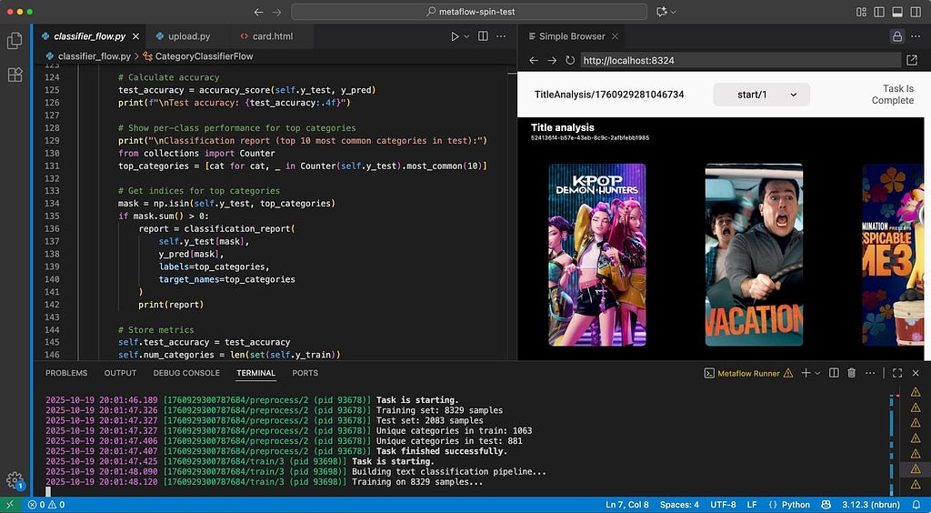


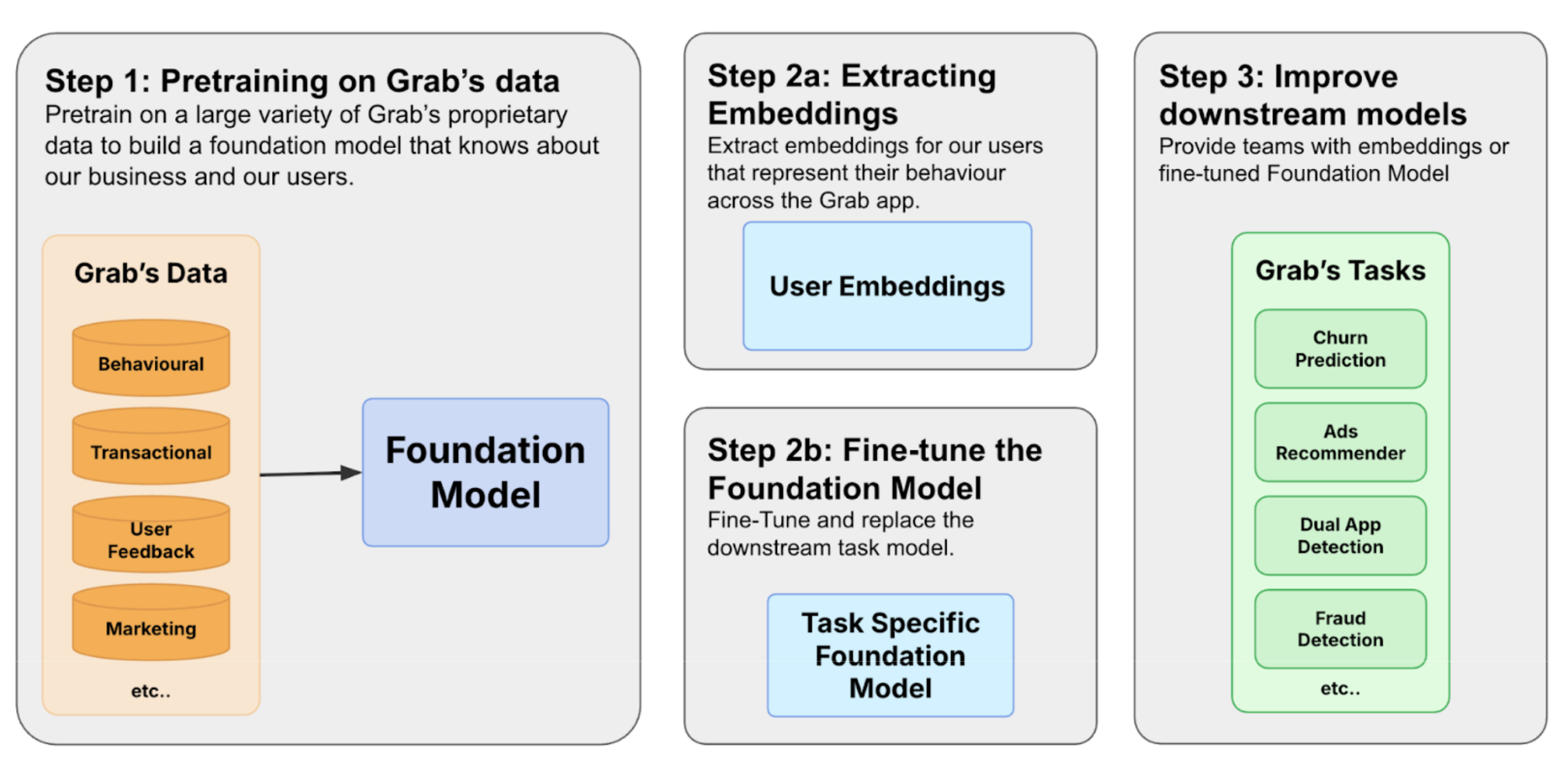
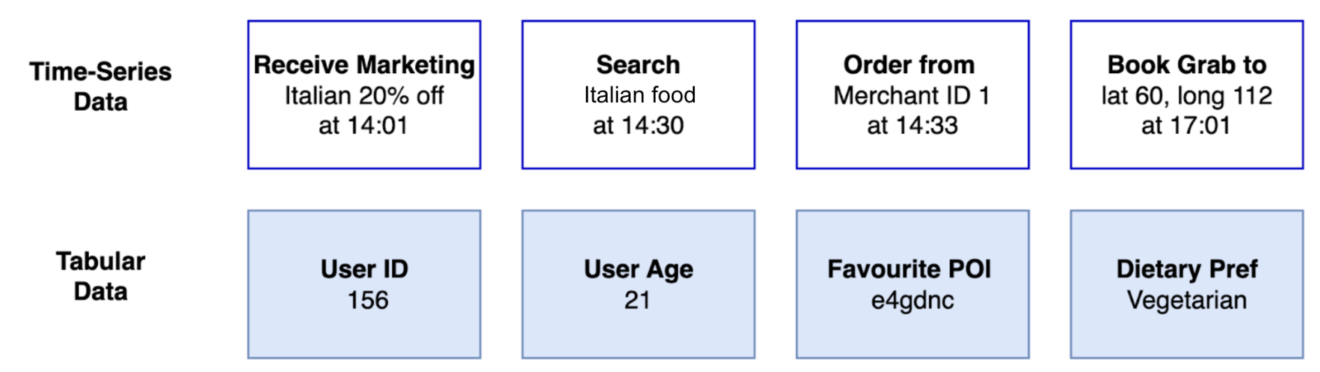
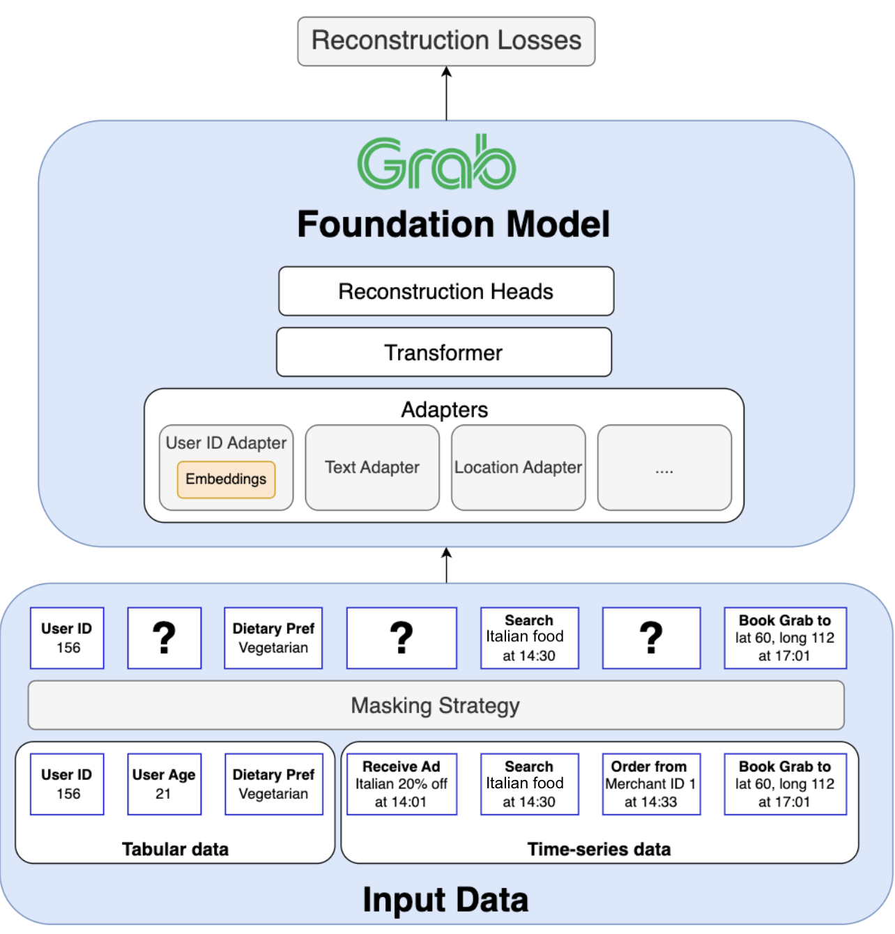

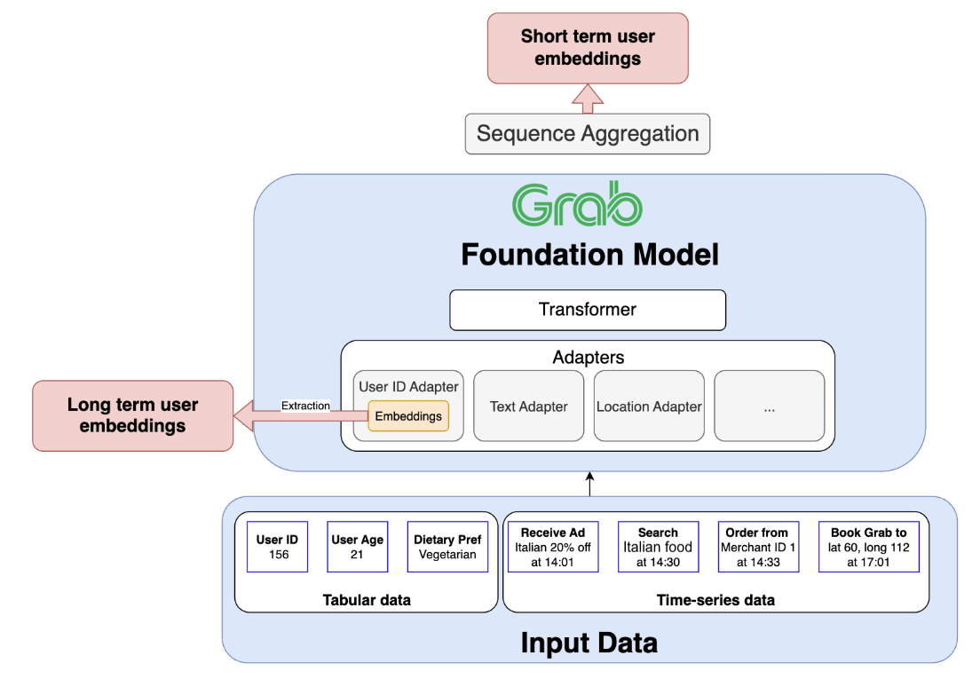
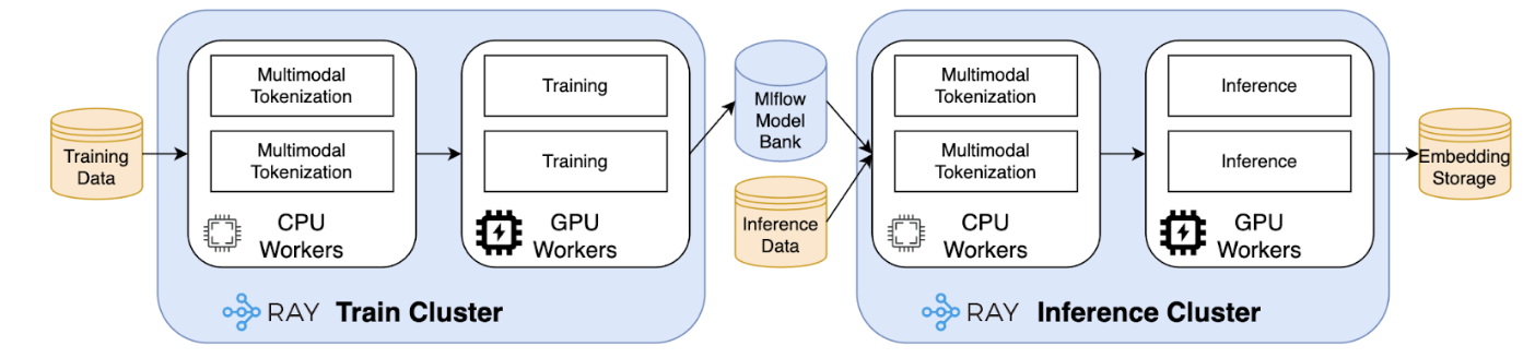


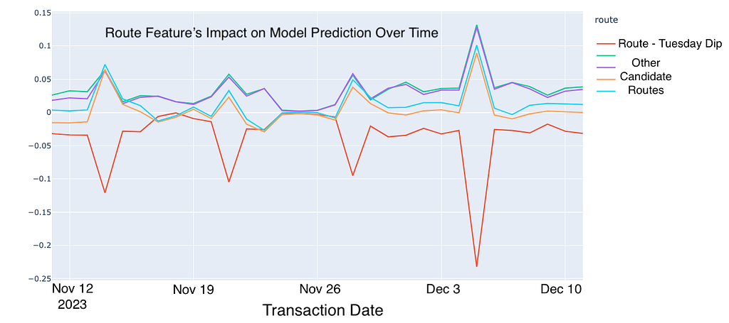
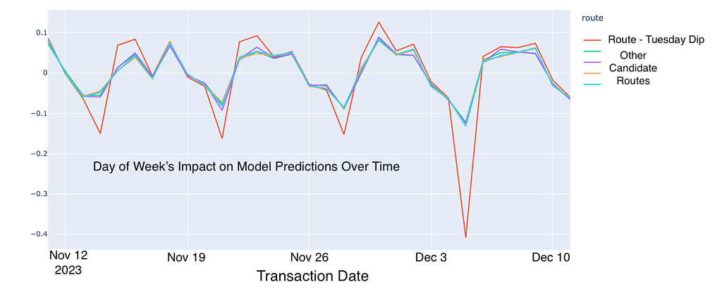

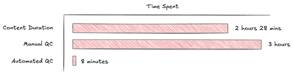


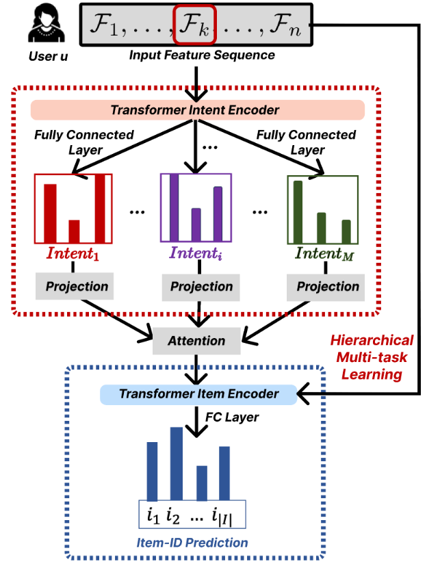

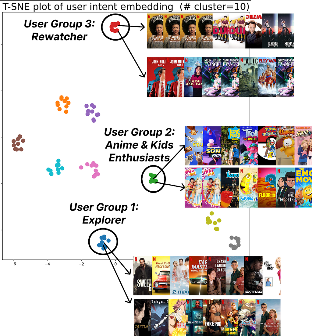
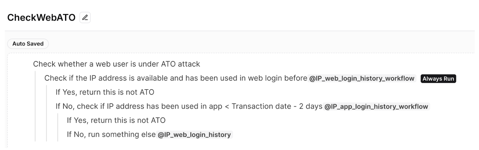

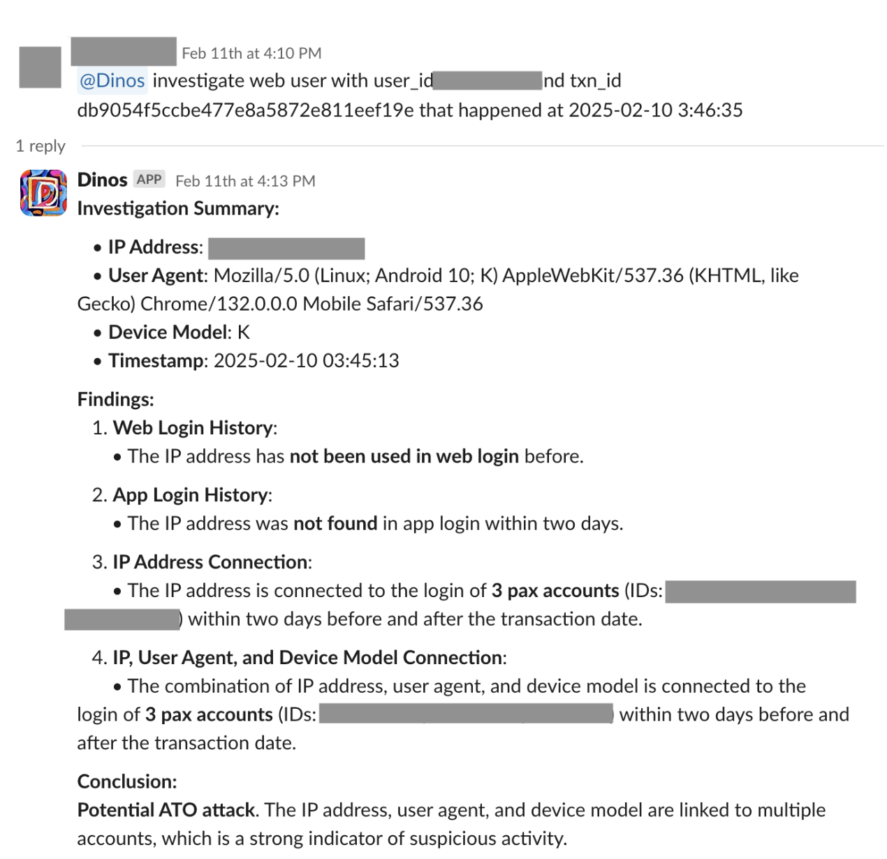
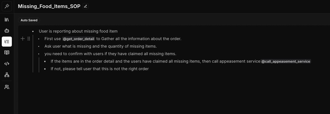


 Kunal Kotwani is a software engineer at Amazon Web Services, focusing on OpenSearch core and vector search technologies. His major contributions include developing storage optimization solutions for both local and remote storage systems that help customers run their search workloads more cost-effectively.
 Navneet Verma is a senior software engineer at AWS OpenSearch . His primary interests include machine learning, search engines and improving search relevancy. Outside of work, he enjoys playing badminton.
 Sorabh Hamirwasia is a senior software engineer at AWS working on the OpenSearch Project. His primary interest include building cost optimized and performant distributed systems.