Tag Archives: reinforcement-learning

Post-Training Generative Recommenders with Advantage-Weighted Supervised Finetuning

Post Syndicated from Netflix Technology Blog original https://netflixtechblog.com/post-training-generative-recommenders-with-advantage-weighted-supervised-finetuning-61a538d717a9

Author: Keertana Chidambaram, Qiuling Xu, Ko-Jen Hsiao, Moumita Bhattacharya

(*The work was done when Keertana interned at Netflix.)

Introduction

This blog focuses on post-training generative recommender systems. Generative recommenders (GRs) represent a new paradigm in the field of recommendation systems (e.g. HSTU, OneRec). These models draw inspiration from recent advancements in transformer architectures used for language and vision tasks. They approach the recommendation problem, including both ranking and retrieval, as a sequential transduction task. This perspective enables generative training, where the model learns by imitating the next event in a sequence of user activities, thereby effectively modeling user behavior over time.

However, a key challenge with simply replicating observed user patterns is that it may not always lead to the best possible recommendations. User interactions are influenced by a variety of factors — such as trends, or external suggestions — and the system’s view of these interactions is inherently limited. For example, if a user tries a popular show but later indicates it wasn’t a good fit, a model that only imitates this behavior might continue to recommend similar content, missing the chance to enhance the user’s experience.

This highlights the importance of incorporating user preferences and feedback, rather than solely relying on observed behavior, to improve recommendation quality. In the context of recommendation systems, we benefit from a wealth of user feedback, which includes explicit signals such as ratings and reviews, as well as implicit signals like watch time, click-through rates, and overall engagement. This abundance of feedback serves as a valuable resource for improving model performance.

Given the recent success of reinforcement learning techniques in post-training large language models, such as DPO and GRPO, this study investigates whether similar methods can be applied to generative recommenders. Ultimately, our goal is to identify both the opportunities and challenges in using these techniques to enhance the quality and relevance of recommendations.

Unlike language models, post-training generative recommenders presents unique challenges. One of the most significant is the difficulty of obtaining counterfactual feedback in recommendation scenarios. The recommendation feedback is generated on-policy — that is, it reflects users’ real-time interactions with the system as they naturally use it. Since a typical user sequence can span weeks or even years of activity, it is impractical to ask users to review or provide feedback on hypothetical, counterfactual experiences. As a result, the absence of counterfactual data makes it challenging to apply post-training methods such as PPO or DPO, which require feedback from counterfactual user sequences.

Furthermore, post-training methods typically rely on a reward model — either implicit or explicit — to guide optimization. The quality of reward models heavily influences the effectiveness of post-training. In the context of recommendation systems, however, reward signals tend to be much noisier. For instance, if we use watch time as an implicit reward, it may not always accurately reflect user satisfaction: a viewer might stop watching a favorite show simply due to time constraints, while finishing a lengthy show doesn’t necessarily indicate genuine enjoyment.

To address these post-training challenges, we introduce a novel algorithm called Advantage-Weighted Supervised Fine-tuning (A-SFT). Our analysis first demonstrates that reward models in recommendation systems often exhibit higher uncertainty due to the issues discussed above. Rather than relying solely on these uncertain reward models, A-SFT combines supervised fine-tuning with the advantage function to more effectively guide post-training optimization. This approach proves especially effective when the reward model has high variance but still provides valuable directional signals. We benchmark A-SFT against four other representative methods, and our results show that A-SFT achieves better alignment between the pre-trained generative recommendation model and the reward model.

In Figure 1, we conceptualize the pros and cons of different post-training paradigms. For example, Online Reinforcement Learning is most useful when the reward model has a good generalization ability, and behavior cloning is suitable when no reward models are available. Using these algorithms under fitting use cases is the key to a successful post-training. For example, over-exploitation of noisy reward models will hurt task performance, as guidance from the reward models can be simply noise. Conversely, not leveraging a good reward model leaves out potential improvements. We find A-SFT fits the sweet point between offline reinforcement learning and behavior cloning, where it benefits from the directional signals in those noisy estimations and is less dependent on the reward accuracy.

Figure 1: The landscape of RL algorithms based on the reward models’ accuracy

Challenges in Post-training for Recommendation

Reinforcement Learning from Human Feedback (RLHF) is the most popular framework for post-training large language models. In this framework, human annotators evaluate and rank different outputs generated by a model. This feedback is then used to train a reward model that predicts how well a model output aligns with human preferences. This reward model then serves as a proxy for human judgment during reinforcement learning, guiding the model to generate outputs that are more likely to be preferred by humans.

While traditional RLHF methods like PPO or DPO are effective for aligning LLMs, there are several challenges in applying them directly to large-scale recommendation systems:

  1. Lack of Counter-factual Observations

As in typical RLHF settings, collecting real-time feedback from a diverse user base across a wide range of items is both costly and impractical. The data in recommendation are generated by the real-time user interests. Any third-party annotators or even the user themselves lack the practical means to evaluate an alternative reality. For example, it is impractical to ask the Netflix users to evaluate hundreds of unseen movies. Consequently, we lack a live environment in which to perform reinforcement learning.

2. Noisy Reward Models

In addition to the limited counter-factual data, the recommendation task itself has a higher randomness by its nature. The recommendation data has less structure than language data. Users choose to watch some shows not because there is a grammar rule that nouns need to follow by the verbs. In fact, the users’ choices usually exhibit a level of permutation invariance, where swapping the order of events in the user history still makes a valid activity sequence. This randomness in the behaviors makes learning a good reward model extremely difficult. Often the reward models we learnt still have a large margin of errors.

Here is an ablation study we did on the reward model performance with O(Millions) users and O(Billions) of tokens. The reward model uses an open-sourced HSTU architecture in the convenience of reproducing this study. We adopt the standard RLHF approach of training a reward model using offline, human-collected feedback. We start by creating a proxy reward, scored on a scale from 1 to 5 in the convenience of understanding. This reward model is co-trained as a shallow reward head on top of the generative recommender. It predicts the reward for the most recently selected title based on a user’s interaction history. To evaluate its effectiveness, we compare the model’s performance against two simple baselines: (1) predicting the next reward as the average reward the user has given in their past interactions, and (2) predicting it as the average reward that all users have assigned to that particular title in previous interactions.

Table 1: Reward model performance metrics

We observe that the model’s predictions do not significantly outperform the simple baselines. This result is intuitive, as a user’s historical interactions typically cover only a small subset of titles, making it difficult to accurately predict their responses to the vast number of unexplored titles in the catalogue. We expect this to be a potential issue for any large recommendation systems where the ratio between explored and unexplored titles is very small.

3. Lack of Logged Policy

In recommendation systems, the policy that generated the logged data is typically unknown and cannot be directly estimated. Offline reinforcement learning methods often rely on Inverse Propensity Scoring (IPS) to debias such data by reweighting interactions according to the logging policy’s action probabilities. However, estimating the logging policy accurately is challenging and prone to error, which can introduce additional biases, and IPS itself is known to suffer from high variance. Consequently, offline RL approaches that depend on IPS are ill-suited for our setting.

Advantage Weighted Supervised Fine Tuning

Given the three challenges outlined above, we propose a new algorithm Advantage-Weighted SFT (A-SFT). It leverages a combination of supervised fine-tuning and advantage reweighting from reinforcement learning. The key observation is as follows. Despite the reward estimation for each individual event having a high uncertainty, we find the estimations of rewards contain directional signals between high-reward and low-reward events. These signals could help better align the model during post-training.

A central factor in this study is the generalization ability of the reward model. Better generalization enables more accurate predictions of user preferences for unseen titles, thereby making exploration more effective. For reward models with moderate to high generalization power, both online RL methods such as PPO and offline RL methods such as CQL can perform effectively. However, in our setting, reward model generalization is worse than the language counterparts’, which makes these algorithms less appropriate. In addition, the use of techniques like inverse propensity scoring (IPS) introduces a heightened risk of high-variance estimates, prompting us to exclude algorithms such as off-policy REINFORCE.

Our proposed method A-SFT does not rely on IPS. With no need of prior knowledge of the logging policy, it can be generally applied to cases where observation of the environments are limited or biased. This is particularly useful to the recommendation setting due to the user feedback loop and distribution shifts with time. Without knowing the logging policy, A-SFT still provides means to control the policy deviation between the current policy and logging policy by tuning the parameter. This design provides essential means to control the learnt bias from uncertain reward models. We show that A-SFT outperforms baseline behavior cloning by directly optimizing observed rewards.

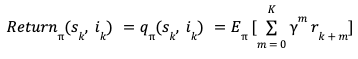
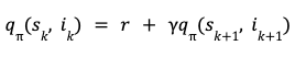
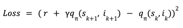
The advantage-weighted SFT algorithm is as follows:

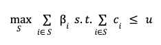
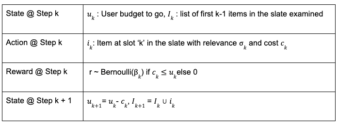
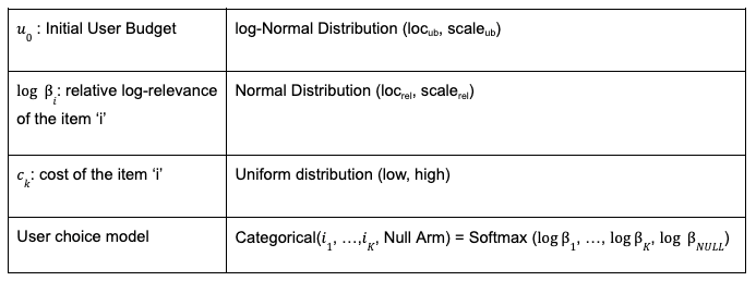
For the results presented in this blog post, we treat the recommendation problem as a contextual bandit, i.e. given a history of user interactions as the context, can we recommend a high reward next title recommendation for the user?

Benchmarks

We compared representative algorithms including PPO, IPO, DPO, CQL and SFT as the baselines:

  1. Reward weighted Behavior Cloning: This benchmark algorithm modifies supervised fine-tuning (SFT) by weighting the loss with the raw rewards of the chosen item instead of weighing the loss with advantage as in the proposed algorithm.
  2. Rejection Sampling Direct Preference Optimization / Identity Preference Optimization (RS DPO/IPO): this is a variant of DPO/IPO where, for each user history x, ​we generate contrasting response pairs by training an ensemble of reward models to estimate confidence intervals for the reward of multiple potential responses y. If the lower bound of the reward confidence interval for one response​ is less than the upper bound for another response, then this pair is used to train DPO/IPO.
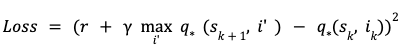
  3. Conservative Q-Learning (CQL): This is a standard offline algorithm that learns a conservative Q function, penalizing overestimation of Q-values, particularly in regions of the state-action space with little or no reward data.
  4. Proximal Policy Optimization (PPO): This is a standard RLHF (Reinforcement Learning from Human Feedback) algorithm that uses reward models as an online environment. PPO learns an advantage function and optimizes the policy to maximize expected reward while maintaining proximity to the initial policy.

We sampled a separate test set of O(Millions) users. This test set is collected on a future date after the training.

Offline Evaluation Results

We evaluate our algorithm on a dataset of high-reward user trajectories. For sake of simplicity, we consider a trajectory to have a high reward if the accumulated reward is higher than the median of the population. We present the following metrics for the held out test dataset:

  1. NDCG@k: This measures the ranking quality of the recommended items up to position k. It accounts for the position of relevant items in the recommendation list, assigning higher scores when relevant items appear higher in the ranking. The gain is discounted logarithmically at lower ranks, and the result is normalized by the ideal ranking (i.e., the best possible ordering of items).
  2. HR@k: This measures the proportion of test cases in which the ground-truth chosen item y appears in the top k recommendations. It is a binary metric per test case (hit or miss) and is averaged over all test cases.
  3. MRR: MRR evaluates the ranking quality by measuring the reciprocal of the rank at which the chosen item appears in the recommendation list. The metric is averaged across all test cases.
  4. Reward Model as A Judge: We use the reward model to evaluate the policy for future user events. We propose to use an ensemble of reward models for the evaluation to increase confidence. The result is based on the discounted reward generated for a few steps. The standard deviation is less than 4%.

We measure the percentage improvement in each metric compared to the baseline, Reward Weighted Behavior Cloning(BC). We notice that advantage weighted SFT shows the largest improvement in metrics, outweighing BC as well as reward model dependent algorithms like CQL, PPO, DPO and IPO.

Our experiments show that advantage weighted SFT is a simple but promising approach for post-training generative recommenders as it deals with the issue of poor reward model generalizations and lack of IPS. More specifically, we find PPO, IPO and DPO achieve a good reward score, but also causes the overfitting from the reward model. Conservative Q-Learning achieves more robust improvements but does not fully capture the potential signals in the reward modeling. A-SFT achieved both better recommendation metrics and reward scores.


Post-Training Generative Recommenders with Advantage-Weighted Supervised Finetuning was originally published in Netflix TechBlog on Medium, where people are continuing the conversation by highlighting and responding to this story.

Reinforcement Learning for Budget Constrained Recommendations

Post Syndicated from Netflix Technology Blog original https://netflixtechblog.com/reinforcement-learning-for-budget-constrained-recommendations-6cbc5263a32a

by Ehtsham Elahi
with
James McInerney, Nathan Kallus, Dario Garcia Garcia and Justin Basilico

Introduction

This writeup is about using reinforcement learning to construct an optimal list of recommendations when the user has a finite time budget to make a decision from the list of recommendations. Working within the time budget introduces an extra resource constraint for the recommender system. It is similar to many other decision problems (for e.g. in economics and operations research) where the entity making the decision has to find tradeoffs in the face of finite resources and multiple (possibly conflicting) objectives. Although time is the most important and finite resource, we think that it is an often ignored aspect of recommendation problems.

In addition to relevance of the recommendations, time budget also determines whether users will accept a recommendation or abandon their search. Consider the scenario that a user comes to the Netflix homepage looking for something to watch. The Netflix homepage provides a large number of recommendations and the user has to evaluate them to choose what to play. The evaluation process may include trying to recognize the show from its box art, watching trailers, reading its synopsis or in some cases reading reviews for the show on some external website. This evaluation process incurs a cost that can be measured in units of time. Different shows will require different amounts of evaluation time. If it’s a popular show like Stranger Things then the user may already be aware of it and may incur very little cost before choosing to play it. Given the limited time budget, the recommendation model should construct a slate of recommendations by considering both the relevance of the items to the user and their evaluation cost. Balancing both of these aspects can be difficult as a highly relevant item may have a much higher evaluation cost and it may not fit within the user’s time budget. Having a successful slate therefore depends on the user’s time budget, relevance of each item as well as their evaluation cost. The goal for the recommendation algorithm therefore is to construct slates that have a higher chance of engagement from the user with a finite time budget. It is important to point out that the user’s time budget, like their preferences, may not be directly observable and the recommender system may have to learn that in addition to the user’s latent preferences.

A typical slate recommender system

We are interested in settings where the user is presented with a slate of recommendations. Many recommender systems rely on a bandit style approach to slate construction. A bandit recommender system constructing a slate of K items may look like the following:

A bandit style recommender system for slate construction

To insert an element at slot k in the slate, the item scorer scores all of the available N items and may make use of the slate constructed so far (slate above) as additional context. The scores are then passed through a sampler (e.g. Epsilon-Greedy) to select an item from the available items. The item scorer and the sampling step are the main components of the recommender system.

Problem formulation

Let’s make the problem of budget constrained recommendations more concrete by considering the following (simplified) setting. The recommender system presents a one dimensional slate (a list) of K items and the user examines the slate sequentially from top to bottom.

A user with a fixed time budget evaluating a slate of recommendations with K items. Item 2 gets the click/response from the user. The item shaded in red falls outside of the user’s time budget.

The user has a time budget which is some positive real valued number. Let’s assume that each item has two features, relevance (a scalar, higher value of relevance means that the item is more relevant) and cost (measured in a unit of time). Evaluating each recommendation consumes from the user’s time budget and the user can no longer browse the slate once the time budget has exhausted. For each item examined, the user makes a probabilistic decision to consume the recommendation by flipping a coin with probability of success proportional to the relevance of the video. Since we want to model the user’s probability of consumption using the relevance feature, it is helpful to think of relevance as a probability directly (between 0 and 1). Clearly the probability to choose something from the slate of recommendations is dependent not only on the relevance of the items but also on the number of items the user is able to examine. A recommendation system trying to maximize the user’s engagement with the slate needs to pack in as many relevant items as possible within the user budget, by making a trade-off between relevance and cost.

Connection with the 0/1 Knapsack problem

Let’s look at it from another perspective. Consider the following definitions for the slate recommendation problem described above

Clearly the abandonment probability is small if the items are highly relevant (high relevance) or the list is long (since the abandonment probability is a product of probabilities). The abandonment option is sometimes referred to as the null choice/arm in bandit literature.

This problem has clear connections with the 0/1 Knapsack problem in theoretical computer science. The goal is to find the subset of items with the highest total utility such that the total cost of the subset is not greater than the user budget. If β_i and c_i are the utility and cost of the i-th item and u is the user budget, then the budget constrained recommendations can be formulated as

0/1 Knapsack formulation for Budget constrained recommendations

There is an additional requirement that optimal subset S be sorted in descending order according to the relevance of items in the subset.

The 0/1 Knapsack problem is a well studied problem and is known to be NP-Complete. There are many approximate solutions to the 0/1 Knapsack problem. In this writeup, we propose to model the budget constrained recommendation problem as a Markov Decision process and use algorithms from reinforcement learning (RL) to find a solution. It will become clear that the RL based solution to budget constrained recommendation problems fits well within the recommender system architecture for slate construction. To begin, we first model the budget constrained recommendation problem as a Markov Decision Process.

Budget constrained recommendations as a Markov Decision Process

In a Markov decision process, the key component is the state evolution of the environment as a function of the current state and the action taken by the agent. In the MDP formulation of this problem, the agent is the recommender system and the environment is the user interacting with the recommender system. The agent constructs a slate of K items by repeatedly selecting actions it deems appropriate at each slot in the slate. The state of the environment/user is characterized by the available time budget and the items examined in the slate at a particular step in the slate browsing process. Specifically, the following table defines the Markov Decision Process for the budget constrained recommendation problem,

Markov Decision Process for Budget constrained recommendations

In real world recommender systems, the user budget may not be observable. This problem can be solved by computing an estimate of the user budget from historical data (e.g. how long the user scrolled before abandoning in the historical data logs). In this writeup, we assume that the recommender system/agent has access to the user budget for sake of simplicity.

The slate generation task above is an episodic task i-e the recommender agent is tasked with choosing K items in the slate. The user provides feedback by choosing one or zero items from the slate. This can be viewed as a binary reward r per item in the slate. Let π be the recommender policy generating the slate and γ be the reward discount factor, we can then define the discounted return for each state, action pair as,

State, Action Value function estimation

The reinforcement learning algorithm we employ is based on estimating this return using a model. Specifically, we use Temporal Difference learning TD(0) to estimate the value function. Temporal difference learning uses Bellman’s equation to define the value function of current state and action in terms of value function of future state and action.

Bellman’s equation for state, action value function

Based on this Bellman’s equation, a squared loss for TD-Learning is,

Loss Function for TD(0) Learning

The loss function can be minimized using semi-gradient based methods. Once we have a model for q, we can use that as the item scorer in the above slate recommender system architecture. If the discount factor γ =0, the return for each (state, action) pair is simply the immediate user feedback r. Therefore q with γ = 0 corresponds to an item scorer for a contextual bandit agent whereas for γ > 0, the recommender corresponds to a (value function based) RL agent. Therefore simply using the model for the value function as the item scorer in the above system architecture makes it very easy to use an RL based solution.

Budget constrained Recommendation Simulation

As in other applications of RL, we find simulations to be a helpful tool for studying this problem. Below we describe the generative process for the simulation data,

Generative model for simulated data

Note that, instead of sampling the per-item Bernoulli, we can alternatively sample once from a categorical distribution with relative relevances for items and a fixed weight for the null arm. The above generative process for simulated data depends on many hyper-parameters (loc, scale etc.). Each setting of these hyper-parameters results in a different simulated dataset and it’s easy to realize many simulated datasets in parallel. For the experiments below, we fix the hyper-parameters for the cost and relevance distributions and sweep over the initial user budget distribution’s location parameter. The attached notebook contains the exact settings of the hyper-parameters used for the simulations.

Metric

A slate recommendation algorithm generates slates and then the user model is used to predict the success/failure of each slate. Given the simulation data, we can train various recommendation algorithms and compare their performance using a simple metric as the average number of successes of the generated slates (referred to as play-rate below). In addition to play-rate, we look at the effective-slate-size as well, which we define to be the number of items in the slate that fit the user’s time budget. As mentioned earlier, one of the ways play-rate can be improved is by constructing larger effective slates (with relevant items of-course) so looking at this metric helps understand the mechanism of the recommendation algorithms.

On-policy learning results

Given the flexibility of working in the simulation setting, we can learn to construct optimal slates in an on-policy manner. For this, we start with some initial random model for the value function, generate slates from it, get user feedback (using the user model) and then update the value function model using the feedback and keep repeating this loop until the value function model converges. This is known as the SARSA algorithm.

The following set of results show how the learned recommender policies behave in terms of metric of success, play-rate for different settings of the user budget distributions’s location parameter and the discount factor. In addition to the play rate, we also show the effective slate size, average number of items that fit within the user budget. While the play rate changes are statistically insignificant (the shaded areas are the 95% confidence intervals estimated using bootstrapping simulations 100 times), we see a clear trend in the increase in the effective slate size (γ > 0) compared to the contextual bandit (γ= 0)

Play-Rate and Effective slate sizes for different User Budget distributions. The user budget distribution’s location is on the same scale of the item cost and we are looking for changes in the metrics as we make changes to the user budget distribution

We can actually get a more statistically sensitive result by comparing the result of the contextual bandit with an RL model for each simulation setting (similar to a paired comparison in paired t-test). Below we show the change in play rate (delta play rate) between any RL model (shown with γ = 0.8 below as an example) and a contextual bandit (γ = 0). We compare the change in this metric for different user budget distributions. By performing this paired comparison, we see a statistically significant lift in play rate for small to medium budget user budget ranges. This makes intuitive sense as we would expect both approaches to work equally well when the user budget is too large (therefore the item’s cost is irrelevant) and the RL algorithm only outperforms the contextual bandit when the user budget is limited and finding the trade-off between relevance and cost is important. The increase in the effective slate size is even more dramatic. This result clearly shows that the RL agent is performing better by minimizing the abandonment probability by packing more items within the user budget.

Paired comparison between RL and Contextual bandit. For limited user budget settings, we see statistically significant lift in play rate for the RL algorithm.

Off-policy learning results

So far the results have shown that in the budget constrained setting, reinforcement learning outperforms contextual bandit. These results have been for the on-policy learning setting which is very easy to simulate but difficult to execute in realistic recommender settings. In a realistic recommender, we have data generated by a different policy (called a behavior policy) and we want to learn a new and better policy from this data (called the target policy). This is called the off-policy setting. Q-Learning is one well known technique that allows us to learn optimal value function in an off-policy setting. The loss function for Q-Learning is very similar to the TD(0) loss except that it uses Bellman’s optimality equation instead

Loss function for Q-Learning

This loss can again be minimized using semi-gradient techniques. We estimate the optimal value function using Q-Learning and compare its performance with the optimal policy learned using the on-policy SARSA setup. For this, we generate slates using Q-Learning based optimal value function model and compare the play-rate with the slates generated using the optimal policy learned with SARSA. Below is result of the paired comparison between SARSA and Q-Learning,

Paired comparison between Q-Learning and SARSA. Play rates are similar between the two approaches but effective slate sizes are very different.

In this result, the change in the play-rate between on-policy and off-policy models is close to zero (see the error bars crossing the zero-axis). This is a favorable result as this shows that Q-Learning results in similar performance as the on-policy algorithm. However, the effective slate size is quite different between Q-Learning and SARSA. Q-Learning seems to be generating very large effective slate sizes without much difference in the play rate. This is an intriguing result and needs a little more investigation to fully uncover. We hope to spend more time understanding this result in future.

Conclusion:

To conclude, in this writeup we presented the budget constrained recommendation problem and showed that in order to generate slates with higher chances of success, a recommender system has to balance both the relevance and cost of items so that more of the slate fits within the user’s time budget. We showed that the problem of budget constrained recommendation can be modeled as a Markov Decision Process and we can find a solution to optimal slate construction under budget constraints using reinforcement learning based methods. We showed that the RL outperforms contextual bandits in this problem setting. Moreover, we compared the performance of On-policy and Off-policy approaches and found the results to be comparable in terms of metrics of success.

Code

Github repo


Reinforcement Learning for Budget Constrained Recommendations was originally published in Netflix TechBlog on Medium, where people are continuing the conversation by highlighting and responding to this story.

Emerging Solutions for Operations Research on AWS

Post Syndicated from Randy DeFauw original https://aws.amazon.com/blogs/architecture/emerging-solutions-for-operations-research-on-aws/

Operations research (OR) uses mathematical and analytical tools to arrive at optimal solutions for complex business problems like workforce scheduling. The mathematical techniques used to solve these problems, such as linear programming and mixed-integer programming, require the use of optimization software (solvers).  There are several popular and powerful solvers available, ranging from commercial options like IBM CPLEX to open-source packages like ORTools. While these solvers incorporate decades of algorithmic expertise and can solve large and complex problems effectively, they have some scalability limitations.

In this post, we’ll describe three alternatives that you can consider for solving OR problems (see Figure 1). None of these are as general purpose as traditional solvers, but they should be on your “emerging technologies” radar.

Figure 1. OR optimization options

Figure 1. OR optimization options

These include:

  1. A traditional solver running on a compute platform
  2. Reinforcement and machine learning (ML) algorithms running on Amazon SageMaker
  3. A quantum computing algorithm running on Amazon Braket. Experiments are collected in Amazon DynamoDB and the results are visualized in Amazon Elasticsearch Service.

A reference problem and solution

Let’s start with a reference problem and solve it with a traditional solver. We’ll tackle an inventory management issue (see Figure 2). We have a sales depot that supplies products for local sales outlets. For the depot’s Region, there are seven weeks of historical sales data for each product. We also know how much each product costs and for how much it can be sold. Finally, we know the overall weekly capacity of the depot. This depends on logistical constraints like the size of the warehouse and transportation availability. This scenario is loosely based on the Grupo Bimbo retailer’s Kaggle competition and dataset.

Figure 2. Sales depot inventory management scenario

Figure 2. Sales depot inventory management scenario

Our job is to place an inventory order to restock our sales depot each week. We quantify our work through a reward function. We want to maximize our revenue:

revenue = (sale price * number of units sold)

(Note that the sample dataset does not include cost of goods sold, only sale price.)

We use these constraints:

total units sold <= depot capacity
0 <= quantity sold of any given item <= forecasted demand for that item

There are many possible solutions to this problem. Using ORTools, we get an average reward (profit) of about $5,700, in about 1,000 simulations.

We can make the scenario slightly more realistic by acknowledging that our sales forecasts are not perfect. After we get the solution from the solver, we can penalize the reward (profit) by subtracting the cost of unsold goods. With this approach, we get a reward of about $2,450.

Solving OR problems with reinforcement learning

An alternative approach to the traditional solver is reinforcement learning (RL). RL is a field of ML that handles problems where the right answer is not immediately known, like playing a game of chess. RL fits our sales depot scenario, because we don’t know how well we will do until after we place the order and are able to view a week of sales activity.

Our sales depot problem resembles a knapsack problem. This is a common OR pattern where we want to fill a container (in this case, our sales depot) with as many items as possible until capacity is reached. Each item has a value (sales price) and a weight (cost). In RL we have to translate this into an observation space, an action space, a state, and a reward (see Figure 3).

The observation space is what our purchasing agent sees. This includes our depot capacity, the sales price, and the forecasted demand. The action space is what our agent can do. In the simplest case, it’s the number of each item to order for the depot, each week. The state is what the agent sees right now, and we model that as the sales results from last week. Finally, the reward function is our profit equation.

One important distinction between OR solvers and RL is that we can’t easily enforce hard constraints in RL. We can limit the amount of an individual product we purchase each week, but we can’t enforce an overall limit on the number of items purchased. We may exceed the capacity of our depot. The simplest way to handle that is to enforce a penalty. There are more sophisticated techniques available, such as interpreting our action as the percentage of budget to spend on each item. But let’s illustrate the simple case here.

Using an RL algorithm from the Ray RLLib package, our reward was $7,000 on average, including penalties for ordering too much of any given item.

Figure 3. Translating OR problem to RL

Figure 3. Translating OR problem to RL

Solving OR problems with machine learning

It’s possible to model a knapsack problem using ML rather than RL in some cases, and there are simple reference implementations available. The design assumes that we know, or can accurately estimate the reward for a given week. With our simple scenario, we can compute the reward using estimates of future sales. We can use this in a custom loss function to train a neural network.

Solving OR problems with quantum computing

Quantum computers are fundamentally different than the computers most of us use. The appeal of quantum computers is that they can tackle some types of problems much more efficiently than standard computers. Quantum computers can, in theory, solve prime number factoring for decryption in orders of magnitude faster than a standard computer. But they are still in their infancy and limited to the size of problem they can handle, due to hardware limitations.

D-Wave Systems, which make some of the types of quantum computers available through Amazon Braket, has a solver called QBSolv. QBSolv works on a specific type of optimization problem called quadratic unconstrained binary optimization (QUBO). It breaks large problems into smaller pieces that a quantum computer can handle. There is a reference pattern for translating a knapsack problem to a QUBO problem.

Running the sales depot problem through QBSolv on Amazon Braket and using a subset of the data, I was able to obtain a reward of $900. When I tried to run on the full dataset, I was not able to complete the decomposition step, likely due to a hardware limitation.

Conclusion

In this blog post, I review OR problems and traditional OR solvers. I then discussed three alternative approaches, RL, ML, and quantum computing. Each of these alternatives has drawbacks and none is a general-purpose replacement for traditional OR solvers.

However, RL and ML are potentially more scalable because you can train those solutions on a cluster of machines, rather than running an OR solver on a single machine. RL agents can also learn from experience, giving them flexibility to handle scenarios that may be difficult to incorporate into an OR solver. Quantum computing solutions are promising but the current state of the art for quantum computers limits their application to small-scale problems at the moment. All of these alternatives can potentially derive a solution more quickly than an OR solver.

Further Reading: