Tag Archives: vmaf

Netflix Video Quality at Scale with Cosmos Microservices

Post Syndicated from Netflix Technology Blog original https://netflixtechblog.com/netflix-video-quality-at-scale-with-cosmos-microservices-552be631c113

by Christos G. Bampis, Chao Chen, Anush K. Moorthy and Zhi Li

Introduction

Measuring video quality at scale is an essential component of the Netflix streaming pipeline. Perceptual quality measurements are used to drive video encoding optimizations, perform video codec comparisons, carry out A/B testing and optimize streaming QoE decisions to mention a few. In particular, the VMAF metric lies at the core of improving the Netflix member’s streaming video quality. It has become a de facto standard for perceptual quality measurements within Netflix and, thanks to its open-source nature, throughout the video industry.

As VMAF evolves and is integrated with more encoding and streaming workflows within Netflix, we need scalable ways of fostering video quality innovations. For example, when we design a new version of VMAF, we need to effectively roll it out throughout the entire Netflix catalog of movies and TV shows. This article explains how we designed microservices and workflows on top of the Cosmos platform to bolster such video quality innovations.

The coupling problem

Until recently, video quality measurements were generated as part of our Reloaded production system. This system is responsible for processing incoming media files, such as video, audio and subtitles, and making them playable on the streaming service. The Reloaded system is a well-matured and scalable system, but its monolithic architecture can slow down rapid innovation. More importantly, within Reloaded, video quality measurements are generated together with video encoding. This tight coupling means that it is not possible to achieve the following without re-encoding:

A) rollout of new video quality algorithms

B) maintaining the data quality of our catalog (e.g. via bug fixes).

Re-encoding the entire catalog in order to generate updated quality scores is an extremely costly solution and hence infeasible. Such coupling problems abound with our Reloaded architecture, and hence the Media Cloud Engineering and Encoding Technologies teams have been working together to develop a solution that addresses many of the concerns with our previous architecture. We call this system Cosmos.

Cosmos is a computing platform for workflow-driven, media-centric microservices. Cosmos offers several benefits as highlighted in the linked blog, such as separation of concerns, independent deployments, observability, rapid prototyping and productization. Here, we describe how we architected the video quality service using Cosmos and how we managed the migration from Reloaded to Cosmos for video quality computations while running a production system.

Video quality as a service

In Cosmos, all video quality computations are performed by an independent microservice called the Video Quality Service (VQS). VQS takes as input two videos: a source and its derivative, and returns back the measured perceptual quality of the derivative. The measured quality could be a single value, in cases where only a single metric’s output is needed (e.g., VMAF), or it could also return back multiple perceptual quality scores, in cases where the request asks for such computation (e.g., VMAF and SSIM).

VQS, like most Cosmos services, consists of three domain-specific and scale-agnostic layers. Each layer is built on top of a corresponding scale-aware Cosmos subsystem. There is an external-facing API layer (Optimus), a rule-based video quality workflow layer (Plato) and a serverless compute layer (Stratum). The inter-layer communication is based on our internally developed and maintained Timestone queuing system. The figure below shows each layer and the corresponding Cosmos subsystem in parenthesis.

An overview of the Video Quality Service (VQS) in Cosmos.
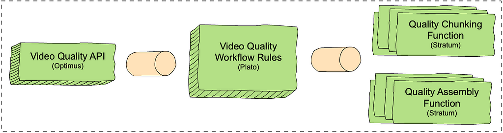
  1. The VQS API layer exposes endpoints: one to request quality measurements (measureQuality) and one to get quality results asynchronously (getQuality).
  2. The VQS workflow layer consists of rules that determine how to measure video quality. Similar to chunk-based encoding, the VQS workflow consists of chunk-based quality calculations, followed by an assembly step. This enables us to use our scale to increase throughput and reduce latencies. The chunk-based quality step computes the quality for each chunk and the assembly step combines the results of all quality computations. For example, if we have two chunks with two and three frames and VMAF scores of [50, 60] and [80, 70, 90] respectively, the assembly step combines the scores into [50, 60, 80, 70, 90]. The chunking rule calls out to the chunk-based quality computation function in Stratum (see below) for all the chunks in the video, and the assembly rule calls out to the assembly function.
  3. The VQS Stratum layer consists of two functions, which perform the chunk-based quality calculation and assembly.

Deep dive into the VQS workflow

The following trace graph from our observability portal, Nirvana, sheds more light on how VQS works. The request provides the source and the derivative whose quality is to be computed and requests that the VQS provides quality scores using VMAF, PSNR and SSIM as quality metrics.

A simplified trace graph from Nirvana.

Here is a step-by-step description of the processes involved:

1. VQS is called using the measureQuality endpoint. The VQS API layer will translate the external request into VQS-specific data models.

2. The workflow is initiated. Here, based on the video length, the throughput and latency requirements, available scale etc., the VQS workflow decides that it will split the quality computation across two chunks and hence, it creates two messages (one for each chunk) to be executed independently by the chunk-based quality computation Stratum function. All three requested quality metrics will be calculated for each chunk.

3. Quality calculation begins for each chunk. The figure does not show the chunk start times separately, however, each chunked quality computation starts and completes (annotated as 3a and 3b) independently based on resource availability.

3b. Plato initiates assembly once all chunked quality computations complete.

4. Assembly begins, with separate invocations to the assembler stratum functions for each metric. As before, the start time for each metric’s assembly can vary. Such separation of computation allows us to fail partially, return early, scale independently depending on metric complexity etc.

4a & 4b. Assembly for two of the metrics (e.g. PSNR and SSIM) is complete.

4c & 5. Assembly for VMAF is complete and the entire workflow is thus completed. The quality results are now available to the caller via the getQuality endpoint.

The above is a simplified illustration of the workflow, however, in practice, the actual design is extremely flexible, and supports a variety of features, including different quality metrics, adaptive chunking strategies, producing quality at different temporal granularities (frame-level, segment level and aggregate) and measuring quality for different use cases, such as measuring quality for different device types (like a phone), SDR, HDR and others.

Living a double life

While VQS is a dedicated video quality microservice that addresses the aforementioned coupling with video encoding, there is another aspect to be addressed. The entire Reloaded system is currently being migrated into Cosmos. This is a big, cross-team effort which means that some applications are still in Reloaded, while others have already made it into Cosmos. How do we leverage VQS, while some applications that consume video quality measurements are still in Reloaded? In other words, how do we manage living a life in both worlds?

A bridge between two worlds

To live such a life, we developed several “bridging” workflows, which allow us to route video quality traffic from Reloaded into Cosmos. Each of these workflows also acts as a translator of Reloaded data models into appropriate Cosmos-service data models. Meanwhile, Cosmos-only workflows can be integrated with VQS without the need for bridging. This allows us to not only operate in both worlds and provide existing video quality features, but also roll out new features ubiquitously (either for Reloaded or Cosmos customer applications).

Living a double life, VQS is at the center of both!

Data conversions as a service

To complete our design, we have to solve one last puzzle. While we have a way to call VQS, the VQS output is designed to avoid the centralized data modeling of Reloaded. For example, VQS relies on the Netflix Media Database (NMDB) to store and index the quality scores, while the Reloaded system uses a mix of non-queryable data models and files. To aid our transition, we introduced another Cosmos microservice: the Document Conversion Service (DCS). DCS is responsible for converting between Cosmos data models and Reloaded data models. Further, DCS also interfaces with NMDB and hence is capable of converting from the data store to Reloaded file-based data and vice-versa. DCS has several other end points that perform similar data conversion when needed so the above described Roman-riding can occur gracefully.

Left: DCS is called to convert the output of VQS into a requested data model. Right: DCS converts Reloaded data models into Cosmos data models before calling VQS.

Where we are now and what’s next

We have migrated almost all of our video quality computations from Reloaded into Cosmos. VQS currently represents the largest workload fueled by the Cosmos platform. Video quality has matured in Cosmos and we are invested in making VQS more flexible and efficient. Besides supporting existing video quality features, all our new video quality features have been developed in VQS. Stay tuned for more details on these algorithmic innovations.

Acknowledgments

This work was made possible with the help of many stunning Netflix colleagues. We would like to thank George Ye and Sujana Sooreddy for their contributions to the Reloaded-Cosmos bridge development, Ameya Vasani and Frank San Miguel for contributing to power up VQS at scale and Susie Xia for helping with performance analysis. Also, the Media Content Playback team, the Media Compute/Storage Infrastructure team and the entire Cosmos platform team that brought Cosmos to life and whole-heartedly supported us in our venture into Cosmos.

If you are interested in becoming a member of our team, we are hiring! Our current job postings can be found here:

https://jobs.netflix.com/jobs/101109705

https://jobs.netflix.com/jobs/127695186

https://jobs.netflix.com/jobs/126802582


Netflix Video Quality at Scale with Cosmos Microservices was originally published in Netflix TechBlog on Medium, where people are continuing the conversation by highlighting and responding to this story.

CAMBI, a banding artifact detector

Post Syndicated from Netflix Technology Blog original https://netflixtechblog.com/cambi-a-banding-artifact-detector-96777ae12fe2

by Joel Sole, Mariana Afonso, Lukas Krasula, Zhi Li, and Pulkit Tandon

Introducing the banding artifacts detector developed by Netflix aiming at further improving the delivered video quality

Banding artifacts can be pretty annoying. But, first of all, you may wonder, what is a banding artifact?

Banding artifact?

You are at home enjoying a show on your brand-new TV. Great content delivered at excellent quality. But then, you notice some bands in an otherwise beautiful sunset scene. What was that? A sci-fi plot twist? Some device glitch? More likely, banding artifacts, which appear as false staircase edges in what should be smoothly varying image areas.

Bands can show up in the sky in that sunset scene, in dark scenes, in flat backgrounds, etc. In any case, we don’t like them, nor should anybody be distracted from the storyline by their presence.

Just a subtle change in the video signal can cause banding artifacts. This slight variation in the value of some pixels disproportionately impacts the perceived quality. Bands are more visible (and annoying) when the viewing conditions are right: large TV with good contrast and a dark environment without screen reflections.

Some examples below. Since we don’t know where and when you are reading this blog post, we exaggerate the banding artifacts, so you get the gist. The first example is from the opening scene of one of our first shows. Check out the sky. Do you see the bands? The viewing environment (background brightness, ambient lighting, screen brightness, contrast, viewing distance) influences the bands’ visibility. You may play with those factors and observe how the perception of banding is affected.

Banding artifacts are also found in compressed images, as in this one we have often used to illustrate the point:

Even the Voyager encountered banding along the way; xkcd 🙂

How annoying is it?

We set up an experiment to measure the perceived quality in the presence of banding artifacts. We asked participants to rate the impact of the banding artifacts on a scale from 0 (unwatchable) to 100 (imperceptible) for a range of videos with different resolutions, bit-rates, and dithering. Participants rated 86 videos in total. Most of the content was banding-prone, while some not. The collected mean opinion scores (MOS) covered the entire scale.

According to usual metrics, the videos in the experiment with perceptible banding should be mid to high-quality (i.e., PSNR>40dB and VMAF>80). However, the experiment scores show something entirely different, as we’ll see below.

You can’t fix it if you don’t know it’s there

Netflix encodes video at scale. Likewise, video quality is assessed at scale within the encoding pipeline, not by an army of humans rating each video. This is where objective video quality metrics come in, as they automatically provide actionable insights into the actual quality of an encode.

PSNR has been the primary video quality metric for decades: it is based on the average pixel distance of the encoded video to the source video. In the case of banding, this distance is tiny compared to its perceptual impact. Consequently, there is little information about banding in the PSNR numbers. The data from the subjective experiment confirms this lack of correlation between PSNR and MOS:

Another video quality metric is VMAF, which Netflix jointly developed with several collaborators and open-sourced on Github. VMAF has become a de facto standard for evaluating the performance of encoding systems and driving encoding optimizations, being a crucial factor for the quality of Netflix encodes. However, VMAF does not specifically target banding artifacts. It was designed with our streaming use case in mind, in particular, to capture the video quality of movies and shows in the presence of encoding and scaling artifacts. VMAF works exceptionally well in the general case, but, like PSNR, lacks correlation with MOS in the presence of banding:

VMAF, PSNR, and other commonly used video quality metrics don’t detect banding artifacts properly and, if we can’t catch the issue, we cannot take steps to fix it. Ideally, our wish list for a banding detector would include the following items:

  • High correlation with MOS for content distorted with banding artifacts
  • Simple, intuitive, distortion-specific, and based on human visual system principles
  • Consistent performance across the different resolutions, qualities, and bit-depths delivered in our service
  • Robust to dithering, which video pipelines commonly introduce

We didn’t find any algorithm in the literature that fit our purposes. So we set out to develop one.

CAMBI

We hand-crafted in a traditional NNN (non-neural network) way an algorithm to meet our requirements. A white box solution derived from first principles with just a few, visually-motivated, parameters: the contrast-aware multiscale banding index (CAMBI).

A block diagram describing the steps involved in CAMBI is shown below. CAMBI operates as a no-reference banding detector taking a (distorted) video as an input and producing a banding visibility score as the output. The algorithm extracts pixel-level maps at multiple scales for frames of the encoded video. Subsequently, it combines these maps into a single index motivated by the human contrast sensitivity function (CSF).

Pre-processing

Each input frame goes through up to three pre-processing steps.

The first step extracts the luma component: although chromatic banding exists, like most past works, we assume that most of the banding can be captured in the luma channel. The second step is converting the luma channel to 10-bit (if the input is 8-bit).

Third, we account for the presence of dithering in the frame. Dithering is intentionally applied noise used to randomize quantization error that is shown to reduce banding visibility. To account for both dithered and non-dithered content, we use a 2×2 filter to smoothen the intensity values to replicate the low-pass filtering done by the human visual system.

Multiscale Banding Confidence

We consider banding detection a contrast-detection problem, and hence banding visibility is majorly governed by the CSF. The CSF itself largely depends on the perceived contrast across a step and the spatial frequency of the steps. CAMBI explicitly accounts for the contrast across pixels by looking at the differences in pixel intensity and does this at multiple scales to account for spatial frequency. This is done by calculating pixel-wise banding confidence at different contrasts and scales, each referred to as a CAMBI map for the frame. Banding confidence computation also considers the sensitivity to change in brightness depending on the local brightness. At the end of this process, twenty CAMBI maps are obtained per frame capturing banding across four contrast steps and five scales.

Spatio-Temporal Pooling

CAMBI maps are spatiotemporally pooled to obtain the final banding index. Spatial pooling is done based on the observation that CAMBI maps belong to the initial linear phase of the CSF. First, pooling is applied in the contrast dimension by keeping the maximum weighted contrast for each position. The result is five maps, one per scale. There is an example of such maps further down in this post.

Since regions with the poorest quality dominate the perceived quality of the video, only a percentage of the pixels, those with the most banding, is considered during spatial pooling for the maps at each scale. The resulting scores per scale are linearly combined with CSF-based weights to derive the CAMBI for each frame.

According to our experiments, CAMBI is temporally stable within a single video shot, so a simple average suffices as a temporal pooling mechanism across frames. However, note that this assumption breaks down for videos with multiple shots with different characteristics.

CAMBI agrees with the subjective assessments

Our results show that CAMBI provides a high correlation with MOS while, as illustrated above, VMAF and PSNR have very little correlation. The table reports two correlation coefficients, namely Spearman Rank Order Correlation (SROCC) and Pearson’s Linear Correlation (PLCC):

The following plot visualizes that CAMBI correlates well with subjective scores and that a CAMBI of around 5 is where banding starts to be slightly annoying. Note that, unlike the two quality metrics, CAMBI correlates inversely with MOS: the higher the CAMBI score is, the more perceptible the banding is, and thus the quality is lower.

Staring at the sunset

We use this sunset as an example of banding and how CAMBI scores it. Below we also show the same sunset with fake colors, so bands pop up even more.

There is no banding on the sea part of the image. In the sky, the size of the bands increases as the distance from the sun increases. The five maps below, one per scale, capture the confidence of banding at different spatial frequencies. These maps are further spatially pooled, accounting for the CSF, giving a CAMBI score of 19 for the frame, which perceptually corresponds to somewhere between ‘annoying’ to ‘very annoying’ banding according to the MOS data.

Open-source and next steps

A banding detection mechanism robust to multiple encoding parameters can help identify the onset of banding in videos and serve as the first step towards its mitigation. In the future, we hope to leverage CAMBI to develop a new version of VMAF that can account for banding artifacts.

We open-sourced CAMBI as a new standalone feature in libvmaf. Similar to VMAF, CAMBI is an organic project expected to be gradually improved over time. We welcome any feedback and contributions.

Acknowledgments

We want to thank Christos Bampis, Kyle Swanson, Andrey Norkin, and Anush Moorthy for the fruitful discussions and all the participants in the subjective tests that made this work possible.


CAMBI, a banding artifact detector was originally published in Netflix TechBlog on Medium, where people are continuing the conversation by highlighting and responding to this story.