Post Syndicated from Antonia Schulze original https://aws.amazon.com/blogs/architecture/field-notes-building-an-automated-image-processing-and-model-training-pipeline-for-autonomous-driving/
In this blog post, we demonstrate how to build an automated and scalable data pipeline for autonomous driving. This solution was built with the goal of accelerating the process of analyzing recorded footage and training a model to improve the experience of autonomous driving.
We will demonstrate the extraction of images from ROS bag file by using Amazon Rekognition to label the images for cataloging, and build a searchable database using Amazon DynamoDB. This is so we can find relevant images for training computer vision Machine Learning (ML) algorithms. Next, we show you how to use the database to find suitable images, create a labeling job with Amazon SageMaker Ground Truth, and train a machine learning model to detect cars. The following diagram shows the architecture for this solution.
Overview of the solution
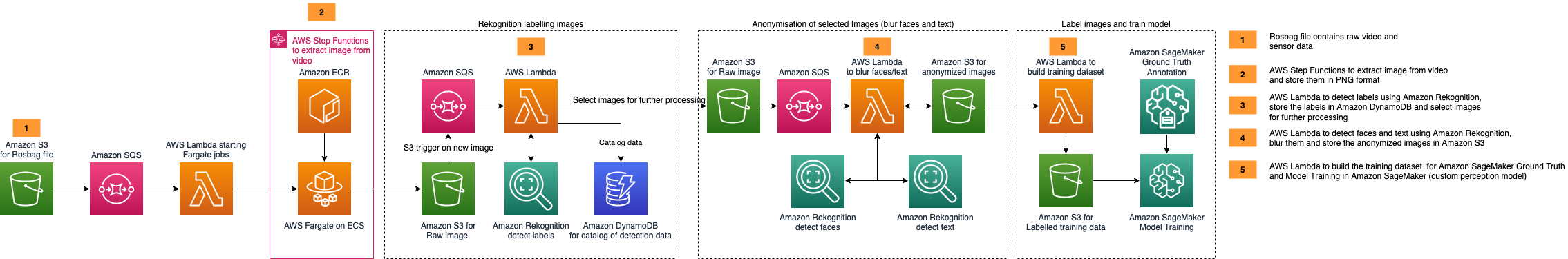
Figure 1 – Architecture Showing how to build an automated Image Processing and Model Training pipeline
Prerequisites
This post uses an AWS Cloud Development Kit (AWS CDK) stack written in Python. Follow the instructions in the CDK Getting Started guide to set up your environment.
Deployment
The full pipeline can be deployed with one command: * `bash deploy.sh deploy true`. We can follow the progress of deployment on the command line, but also in the CloudFormation section of the AWS console. Once the pipeline is deployed, we must upload bag files to the rosbag-ingest bucket to launch the pipeline. Once the pipeline has finished, we can clone the repository to the SageMaker Notebook instance ros-bag-demo-notebook.
Walkthrough
- The Robot Operating System (ROS) is a collection of open source middleware, which provides tools and libraries for building robotic systems. The middleware uses a Publish/Subscribe (pub/sub) architecture, which can be used for the transportation of sensor data to any software modules, which need to operate on that data.
- Each sensor publishes its data as a topic, and then any module which needs that data subscribes to that topic.
- This Pub/Sub architecture lends itself well to recording data from multiple sensors of varying modalities (camera, LIDAR, RADAR) into a single file which can be replayed for testing and diagnostic purposes. ROS supports this capability with its ROS bag module which stores data in an ROS bag format file.
- An ROS bag file includes a collection of topics, each with a set of time-stamped messages. These files can be replayed on an ROS system, with the timestamps, ensuring that messages are published to the topics in real time and the order they were recorded.
- The input for this example is a set of ROS bag files, each one is approximately 10 GB.
- To extract the image data from our input ROS bag files, you create a Docker container based on an ROS image.
- You then create an ROS launch configuration file to extract images to .png files based on the ROS bag tutorial instructions. The Docker container is stored in an Amazon Elastic Container Registry (Amazon ECR), ready to run as an AWS Fargate task.
AWS Fargate is a serverless compute engine for containers that work with both Amazon Elastic Container Service (Amazon ECS) and Amazon Elastic Kubernetes Service (EKS). By using Fargate, we can create and run the Docker containers with our ROS environment, and have many containers running in parallel with each processing a single ROS bag file.
When you have the individual images, you need a way to assess their contents to build a searchable image catalog. This objective allows ML data scientists to search through the recorded images to find, for example, images containing pedestrians. The catalog can also be extended with data from other sources, such as weather data, location data, and so forth. You use Amazon Rekognition to process the images, and it helps add image and video analysis to your applications. When you provide an image or video to the Amazon Rekognition API, the service identifies objects, people, text, scenes, and activities. By requesting that Amazon Rekognition label each image, you receive a large amount of information to catalog the image.
The image ingestion pipeline is largely event driven. Many of the AWS services you use have limits on job concurrency and API access rates. To resolve these issues, you place all events into an Amazon Simple Queue Service (Amazon SQS) queue, invoke a Lambda function on queue, and make the appropriate API call (for example, Amazon Rekognition DetectLabels). If the API call is successful, you delete the message from the queue, otherwise (for example, the rate is exceeded) you exit the Lambda function and the message will be returned to the queue. One benefit is that when service limits change, depending on the account configuration or Region, the pipeline will automatically scale to accommodate these changes.
- The pipeline is launched when an ROS bag file is uploaded to the Amazon Simple Storage Service (Amazon S3) bucket which has been configured to post an object creation event to an SQS queue.
- A Lambda function is invoked from the SQS queue and it starts a Step Functions step, which runs our dockerized container on a Fargate cluster. An extracted image is stored in an S3 bucket, which invokes a second SQS queue to start a Lambda function. The Lambda function calls the DetectLabels function of the Amazon Rekognition API which, returns labels for everything that Amazon Rekognition can detect in the scene.
- This also includes the confidence level for each label. The labels and confidence scores are stored in a DynamoDB data catalog table. You can query all images for specific objects that you are interested in and filter to create subsets that are of interest.
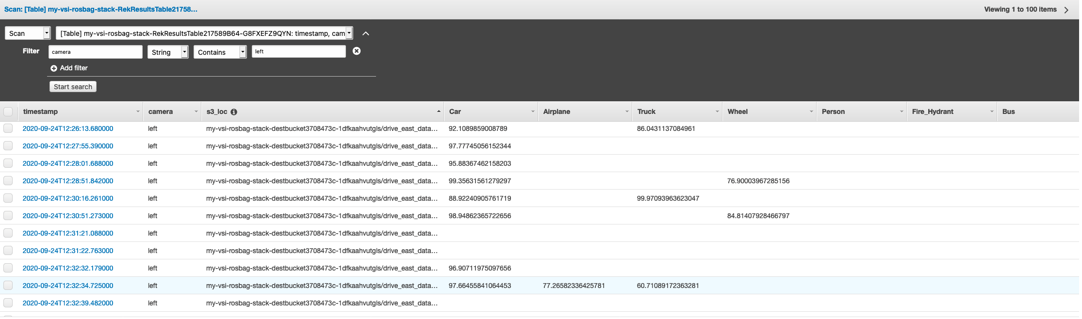
Figure 2 – DynamoDB table containing detected objects and confidence scores
Because you will use a public workforce for labeling in the next section, you will need to create anonymized versions of images where faces and license plates are blurred out. Amazon Rekognition has a DetectFaces API call to find any faces in the image. There is no corresponding call for detecting license plates, so you detect all text in the image with the DetectText API. Use the write of the .json output file to invoke a Lambda function which calls the Amazon Rekognition APIs and blurs the relevant Regions before saving them to S3.
Image labeling with Amazon SageMaker Ground Truth
Since the images are now stored in their raw and anonymized format we can start the data labeling step. We will sample the images we want to label. The data catalog in DynamoDB lets you query the table based on your parameters and sub-area you want to optimize your model on. For example, you could query the DynamoDB table for images having a crowd of pedestrians and specifically label these images and allow your model to improve in these particular circumstances. Once we have identified the images of interest, we can copy them to a specific S3 folder and start the SageMaker Ground Truth job on an object detection task. You can find a detailed blog post on streamlining data for object detection in Amazon SageMaker Ground Truth.
The result of a SageMaker Ground Truth job is a manifest file containing the S3 Path, bounding box coordinates, and class labels (per image). This is automatically uploaded to S3. We need to replace the anonymized images with the raw image S3 Path since we want to train the model on raw images. We have provided you a sample manifest file in the repository and you can follow along the blogpost with the Jupyter Notebook provided in `object-detection/Transfer-Learning.iypnb`. First, we can verify that the annotations are high quality by viewing the following sample image.
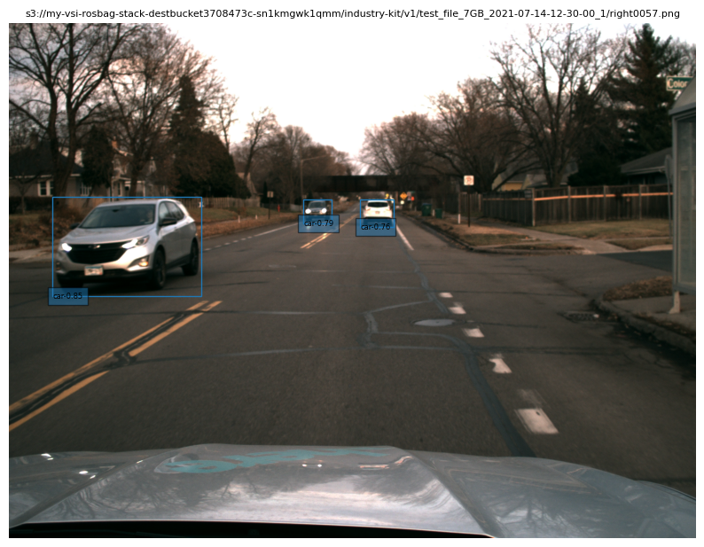
Figure 3 – Visualization of annotations from SageMaker Ground Truth job
Fine-tune a GluonCV model with SageMaker Script Mode
The ML technique transfer learning allows us to use neural networks that have previously been trained on large datasets of similar applications, and fine-tune them based on a smaller custom annotated data. Frameworks such as GluonCV provide a model zoo for object detection, that allows us to have a quick access to these pre-trained models. In this case, we have selected a YOLOv3 model that has been pre-trained on the COCO dataset. Based on empirical analysis, other networks such as Faster-RCNN outperform YOLOv3, but tend to have slower inference times as measured in frames per second, which is a key aspect for real-time applications.
The preferred object detection format for GluonCV is based on .lst file format, and converts to the RecordIO design, providing faster disk access and compact storage. GluonCV provides a tutorial on how to convert a .lst file format into a RecordIO file.
To train a customized neural network we will use Amazon SageMaker Script Mode, allowing us to use your own training algorithms and the straightforward SageMaker UI.
from sagemaker import get_execution_role
sagemaker_session = sagemaker.Session()
role = get_execution_role()
s3_output_path = "s3://<path to bucket where model weights will be saved>/"

model_estimator = MXNet(
    entry_point="train_yolov3.py",
    role=role,
    train_instance_count=1,
    train_instance_type="ml.p3.8xlarge",
    framework_version="1.8.0",
    output_path=s3_output_path,
    py_version="py37"
)

model_estimator.fit("s3://<bucket path for train and validation record-io files>/")
Hyperparameter optimization on SageMaker
While training neural networks, there are many parameters that can be optimized to the use case and the custom dataset. We refer to this as automatic model tuning in SageMaker or hyperparameter optimization. SageMaker launches multiple training jobs with a unique combination of hyperparameters, and search for the configuration achieving the highest mean average precision (mAP) on our held-out test data.
hyperparameter_ranges = {
    "lr": ContinuousParameter(0.001, 0.1),
    "wd": ContinuousParameter(0.0001, 0.001),
    "batch-size": CategoricalParameter([8, 16])
    }
metric_definitions = [
    {"Name": "val:car mAP", "Regex": "val:mAP=(.*?),"},
    {"Name": "test:car mAP", "Regex": "test:mAP=(.*?),"},
    {"Name": "BoxCenterLoss", "Regex": "BoxCenterLoss=(.*?),"},
    {"Name": "ObjLoss", "Regex": "ObjLoss=(.*?),"},
    {"Name": "BoxScaleLoss", "Regex": "BoxScaleLoss=(.*?),"},
    {"Name": "ClassLoss", "Regex": "ClassLoss=(.*?),"},
]
objective_metric_name = "val:car mAP"

hpo_tuner = HyperparameterTuner(
    model_estimator,
    objective_metric_name,
    hyperparameter_ranges,
    metric_definitions,
    max_jobs=10,  # maximum jobs that should be ran
    max_parallel_jobs=2
)

hpo_tuner.fit("s3://<bucket path for train and validation record-io files>/")
Model compilation
Although we don’t have hard constraints for a model environment when training in the cloud, we should mind the production environment when running inference with trained models: no powerful GPUs and limited storage are common challenges. Fortunately, Amazon SageMaker Neo allows you to train once and run anywhere in the cloud and at the edge, while reducing the memory footprint of your model.
best_estimator = hpo_tuner.best_estimator()
compiled_model = best_estimator.compile_model(
    target_instance_family="ml_c4",
    role=role,
    input_shape={"data": [1, 3, 512, 512]},
    output_path=s3_output_path,
    framework="mxnet",
    framework_version="1.8",
    env={"MMS_DEFAULT_RESPONSE_TIMEOUT": "500"}
)
Deploying the model
Deploying a model requires a few additional lines of code for hosting.
from sagemaker.serializers import JSONSerializer
from sagemaker.deserializers import JSONDeserializer

predictor = compiled_model.deploy(
initial_instance_count=1, instance_type="ml.c4.xlarge", endpoint_name="YOLO-DEMO-endpoint", deserializer=JSONDeserializer(),serializer=JSONSerializer()
)
Run inference
Once the model is deployed with an endpoint, we can test some inference. As the model has been trained on 512×512 pixel images, we need to format inference images respectively, before serializing the data and making a prediction request to the SageMaker endpoint.
import PIL.Image
import numpy as np
test_image = PIL.Image.open("test.png")
test_image = np.asarray(test_image.resize((512, 512)))
endpoint_response = predictor.predict(test_image)
We can then visualize the response and show the confidence score associated with the prediction on the test image.
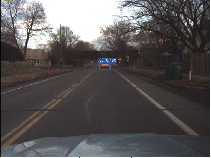
Figure 4 – Visualization of the response and confidence score associated with the prediction on the test image.
Clean Up
To clean up the deployment you should run bash deploy.sh destroy false. In Addition to that, you also need to delete the SageMaker Endpoint. Some resources like S3 buckets and DynamoDB tables must be manually emptied and deleted through the console to be fully removed.
Conclusion
This post described how to extract images at large scale from ROS bag files and label a subset of them with SageMaker Ground Truth. With this labeled training dataset, we fine-tuned an object detection neural network using SageMaker Script Mode. To deploy the model in the autonomous driving vehicle, we compiled the model with SageMaker Neo, reducing the storage size and optimizing the model graph on the specific hardware. Finally, you ran some test inference predictions and visualized them in a SageMaker Notebook. You can find the code for this blog post in this GitHub repository.