Tag Archives: Amazon SageMaker Ground Truth

AWS Week in Review – June 27, 2022

Post Syndicated from Danilo Poccia original https://aws.amazon.com/blogs/aws/aws-week-in-review-june-27-2022/

This post is part of our Week in Review series. Check back each week for a quick roundup of interesting news and announcements from AWS!

It’s the beginning of a new week, and I’d like to start with a recap of the most significant AWS news from the previous 7 days. Last week was special because I had the privilege to be at the very first EMEA AWS Heroes Summit in Milan, Italy. It was a great opportunity of mutual learning as this community of experts shared their thoughts with AWS developer advocates, product managers, and technologists on topics such as containers, serverless, and machine learning.

Participants at the EMEA AWS Heroes Summit 2022

Last Week’s Launches
Here are the launches that got my attention last week:

Amazon Connect Cases (available in preview) – This new capability of Amazon Connect provides built-in case management for your contact center agents to create, collaborate on, and resolve customer issues. Learn more in this blog post that shows how to simplify case management in your contact center.

Many updates for Amazon RDS and Amazon AuroraAmazon RDS Custom for Oracle now supports Oracle database 12.2 and 18c, and Amazon RDS Multi-AZ deployments with one primary and two readable standby database instances now supports M5d and R5d instances and is available in more Regions. There is also a Regional expansion for RDS Custom. Finally, PostgreSQL 14, a new major version, is now supported by Amazon Aurora PostgreSQL-Compatible Edition.

AWS WAF Captcha is now generally available – You can use AWS WAF Captcha to block unwanted bot traffic by requiring users to successfully complete challenges before their web requests are allowed to reach resources.

Private IP VPNs with AWS Site-to-Site VPN – You can now deploy AWS Site-to-Site VPN connections over AWS Direct Connect using private IP addresses. This way, you can encrypt traffic between on-premises networks and AWS via Direct Connect connections without the need for public IP addresses.

AWS Center for Quantum Networking – Research and development of quantum computers have the potential to revolutionize science and technology. To address fundamental scientific and engineering challenges and develop new hardware, software, and applications for quantum networks, we announced the AWS Center for Quantum Networking.

Simpler access to sustainability data, plus a global hackathon – The Amazon Sustainability Data Initiative catalog of datasets is now searchable and discoverable through AWS Data Exchange. As part of a new collaboration with the International Research Centre in Artificial Intelligence, under the auspices of UNESCO, you can use the power of the cloud to help the world become sustainable by participating to the Amazon Sustainability Data Initiative Global Hackathon.

For a full list of AWS announcements, be sure to keep an eye on the What’s New at AWS page.

Other AWS News
A couple of takeaways from the Amazon re:MARS conference:

Amazon CodeWhisperer (preview) – Amazon CodeWhisperer is a coding companion powered by machine learning with support for multiple IDEs and languages.

Synthetic data generation with Amazon SageMaker Ground TruthGenerate labeled synthetic image data that you can combine with real-world data to create more complete training datasets for your ML models.

Some other updates you might have missed:

AstraZeneca’s drug design program built using AWS wins innovation award – AstraZeneca received the BioIT World Innovative Practice Award at the 20th anniversary of the Bio-IT World Conference for its novel augmented drug design platform built on AWS. More in this blog post.

Large object storage strategies for Amazon DynamoDB – A blog post showing different options for handling large objects within DynamoDB and the benefits and disadvantages of each approach.

Amazon DevOps Guru for RDS under the hoodSome details of how DevOps Guru for RDS works, with a specific focus on its scalability, security, and availability.

AWS open-source news and updates – A newsletter curated by my colleague Ricardo to bring you the latest open-source projects, posts, events, and more.

Upcoming AWS Events
It’s AWS Summits season and here are some virtual and in-person events that might be close to you:

On June 30, the AWS User Group Ukraine is running an AWS Tech Conference to discuss digital transformation with AWS. Join to learn from many sessions including a fireside chat with Dr. Werner Vogels, CTO at Amazon.com.

That’s all from me for this week. Come back next Monday for another Week in Review!

Danilo

New – Amazon SageMaker Ground Truth Now Supports Synthetic Data Generation

Post Syndicated from Antje Barth original https://aws.amazon.com/blogs/aws/new-amazon-sagemaker-ground-truth-now-supports-synthetic-data-generation/

Today, I am happy to announce that you can now use Amazon SageMaker Ground Truth to generate labeled synthetic image data.

Building machine learning (ML) models is an iterative process that, at a high level, starts with data collection and preparation, followed by model training and model deployment. And especially the first step, collecting large, diverse, and accurately labeled datasets for your model training, is often challenging and time-consuming.

Let’s take computer vision (CV) applications as an example. CV applications have come to play a key role in the industrial landscape. They help improve manufacturing quality or automate warehouses. Yet, collecting the data to train these CV models often takes a long time or can be impossible.

As a data scientist, you might spend months collecting hundreds of thousands of images from the production environments to make sure you capture all variations in data the model will come across. In some cases, finding all data variations might even be impossible, for example, sourcing images of rare product defects, or expensive, if you have to intentionally damage your products to get those images.

And once all data is collected, you need to accurately label the images, which is often a struggle in itself. Manually labeling images is slow and open to human error, and building custom labeling tools and setting up scaled labeling operations can be time-consuming and expensive. One way to mitigate this data challenge is by adding synthetic data to the mix.

Advantages of Combining Real-World Data with Synthetic Data
Combining your real-world data with synthetic data helps to create more complete training datasets for training your ML models.

Synthetic data itself is created by simple rules, statistical models, computer simulations, or other techniques. This allows synthetic data to be created in enormous quantities and with highly accurate labels for annotations across thousands of images. The label accuracy can be done at a very fine granularity, such as on a sub-object or pixel level, and across modalities. Modalities include bounding boxes, polygons, depth, and segments. Synthetic data can also be generated for a fraction of the cost, especially when compared to remote sensing imagery that otherwise relies on satellite, aerial, or drone image collection.

If you combine your real-world data with synthetic data, you can create more complete and balanced data sets, adding data variety that real-world data might lack. With synthetic data, you have the freedom to create any imagery environment, including edge cases that might be difficult to find and replicate in real-world data. You can customize objects and environments with variations, for example, to reflect different lighting, colors, texture, pose, or background. In other words, you can “order” the exact use case you are training your ML model for.

Now, let me show you how you can start sourcing labeled synthetic images using SageMaker Ground Truth.

Get Started on Your Synthetic Data Project with Amazon SageMaker Ground Truth
To request a new synthetic data project, navigate to the Amazon SageMaker Ground Truth console and select Synthetic data.

Amazon SageMaker Ground Truth Synthetic Data

Then, select Open project portal. In the project portal, you can request new projects, monitor projects that are in progress, and view batches of generated images once they become available for review. To initiate a new project, select Request project.

Amazon SageMaker Ground Truth Synthetic Data Project Portal

Describe your synthetic data needs and provide contact information.

Request a synthetic data project

After you submit the request form, you can check your project status in the project dashboard.

Amazon SageMaker Ground Truth Synthetic Data Project Created

In the next step, an AWS expert will reach out to discuss your project requirements in more detail. Upon review, the team will share a custom quote and project timeline.

If you want to continue, AWS digital artists will start by creating a small test batch of labeled synthetic images as a pilot production for you to review.

They collect your project inputs, such as reference photos and available 2D and 3D assets. The team then customizes those assets, adds the specified inclusions, such as scratches, dents, and textures, and creates the configuration that describes all the variations that need to be generated.

They can also create and add new objects based on your requirements, configure distributions and locations of objects in a scene, as well as modify object size, shape, color, and surface texture.

Once the objects are prepared, they are rendered using a photorealistic physics engine, capturing an image of the scene from a sensor that is placed in the virtual world. Images are also automatically labeled. Labels include 2D bounding boxes, instance segmentation, and contours.

You can monitor the progress of the data generation jobs on the project detail page. Once the pilot production test batch becomes available for review, you can spot-check the images and provide feedback for any rework that might be required.

Review available batches of synthetic data

Select the batch you want to review and View details
Sample batch of synthetic data in Amazon SageMaker Ground Truth

In addition to the images, you will also receive output image labels, metadata such as object positions, and image quality metrics as Amazon SageMaker compatible JSON files.

Synthetic Image Fidelity and Diversity Report
With each available batch of images, you also receive a synthetic image fidelity and diversity report. This report provides image and object level statistics and plots that help you make sense of the generated synthetic images.

The statistics are used to describe the diversity and the fidelity of the synthetic images and compare them with real images. Examples of the statistics and plots provided are the distributions of object classes, object sizes, image brightness, and image contrast, as well as the plots evaluating the indistinguishability between synthetic and real images.

Synthetic Image Fidelity and Diversity Report

Once you approve the pilot production test batch, the team will move to the production phase and start generating larger batches of labeled synthetic images with your desired label types, such as 2D bounding boxes, instance segmentation, and contours. Similar to the test batch, each production batch of images will be made available for you together with the image fidelity and diversity report to spot-check, accept, or reject.

All images and artifacts will be available for you to download from your S3 bucket once final production is complete.

Availability
Amazon SageMaker Ground Truth synthetic data is available in US East (N. Virginia). Synthetic data is priced on a per-label basis. You can request a custom quote that is tailored to your specific use case and requirements by filling out the project requirement form.

Learn more about SageMaker Ground Truth synthetic data on our Amazon SageMaker Data Labeling page.

Request your synthetic data project through the Amazon SageMaker Ground Truth console today!

— Antje

Serverless Architecture for a Structured Data Mining Solution

Post Syndicated from Uri Rotem original https://aws.amazon.com/blogs/architecture/serverless-architecture-for-a-structured-data-mining-solution/

Many businesses have an essential need for structured data stored in their own database for business operations and offerings. For example, a company that produces electronics may want to store a structured dataset of parts. This requires the following properties: color, weight, connector type, and more.

This data may already be available from external sources. In many cases, one source is sufficient. But often, multiple data sources from different vendors must be incorporated. Each data source might have a different structure for the same data field, which is problematic. Achieving one unified structure from variable sources can be difficult, and is a classic data mining problem.

We will break the problem into two main challenges:

  1. Locate and collect data. Collect from multiple data sources and load data into a data store.
  2. Unify the collected data. Since the collected data has no constraints, it might be stored in different structures and file formats. To use the collected data, it must be unified by performing an extract, transform, load (ETL) process. This matches the different data sources and creates one unified data store.

In this post, we demonstrate a pipeline of services, built on top of a serverless architecture that will handle the preceding challenges. This architecture supports large-scale datasets. Because it is a serverless solution, it is also secure and cost effective.

We use Amazon SageMaker Ground Truth as a tool for classifying the data, so that no custom code is needed to classify different data sources.

Data mining and structuring

There are three main steps to explore in order to solve these challenges:

  1. Collect the data – Data mine from different sources
  2. Map the data – Construct a dictionary of key-value pairs without writing code
  3. Structure the collected data – Enrich your dataset with a unified collection of data that was collected and mapped in steps 1 and 2

Following is an example of a use case and solution flow using this architecture:

  • In this scenario, a company must enrich an empty data base with items and properties, see Figure 1.
Figure 1. Company data before data mining

Figure 1. Company data before data mining

  • Data will then be collected from multiple data sources, and stored in the cloud, as shown in Figure 2.
Figure 2. Collecting the data by SKU from different sources

Figure 2. Collecting the data by SKU from different sources

  • To unify different property names, SageMaker Ground Truth is used to label the property names with a list of properties. The results are stored in Amazon DynamoDB, shown in Figure 3.
Figure 3. Mapping the property names to match a unified name

Figure 3. Mapping the property names to match a unified name

  • Finally, the database is populated and enriched by the mapped properties from the different data sources. This can be iterated with new sources to further enrich the data base, see Figure 4.
Figure 4. Company data after data mining, mapping, and structuring

Figure 4. Company data after data mining, mapping, and structuring

1. Collect the data

Using this serverless architecture illustrated in Figure 5, your teams can minimize the effort and cost. You’ll be able to handle large-scale datasets to collect and store the data required for your business.

Figure 5. Serverless architecture for parallel data collection

Figure 5. Serverless architecture for parallel data collection

We use Amazon S3 as it is a highly scalable and durable object storage service, and can store the original dataset. It will initiate an event that will invoke a Lambda function to start a state machine, using the original dataset as its input.

AWS Step Functions are used to orchestrate the process of preparing the dataset for parallel scraping of the items. It will automatically manage the queue of items to be processed when the dataset is large. Step Functions ensures visibility of the process, reports errors, and decouples the compute-intensive scraping operation per item.

The state machine has two steps:

  1. ETL the data to clean and standardize it. Store each item in Amazon DynamoDB, a fast and flexible NoSQL database service for any scale. The ETL function will create an array of all the items identifiers. The identifier is a unique describer of the item, such as manufacturer ID and SKU.
  2. Using the Map functionality of Step Functions, a Lambda function will be invoked for each item. This runs all your scrapers for that item and stores the results in an S3 bucket.

This solution requires custom implementation of only these two functions, according to your own dataset and scraping sources. The ETL Lambda function will contain logic needed to transform your input into an array of identifiers. The scraper Lambda function will contain logic to locate the data in the source and then store it.

Scraper function flow

For each data source, write your own scraper. The Lambda function can run them sequentially.

  1. Use the identifier input to locate the item in each one of the external sources. The data source can be an API, a webpage, a PDF file, or other source.
    • API: Collecting this data will be specific to the interface provided.
    • Webpages: Data is collected with custom code. There are open source libraries that are popular for this task, such as Beautiful Soup.
    • PDF files: Consider using Amazon Textract. Amazon Textract will give you key-value pairs and table analysis.
  2. Transform the response to key-value pairs as part of the scraper logic.
  3. Store the key-value pairs in a sub folder of the scraper responses S3 bucket, and name it after that data source.

2. Mapping the responses

Figure 6. Pipeline for property mapping

Figure 6. Pipeline for property mapping

This pipeline is initiated after the data is collected. It creates a labeling job of Named Entity Recognition, with a pre-defined set of labels. The labeling work will be split among your Workforces. When the job is completed, the output manifest file for named entity recognition is used for the final ETL Lambda. This manually locates the labeling key and values detected by your workforce, and places the results in a reusable mapping table in DynamoDB.

Services used:

Amazon SageMaker Ground Truth is a fully managed data labeling service that helps you build highly accurate training datasets for machine learning (ML). By using Ground Truth, your teams can unify different data sources to match each other, so they can be identified and used in your applications.

Figure 7. Example of one line item being labeled by one of the Workforce team members

Figure 7. Example of one line item being labeled by one of the Workforce team members

3. Structure the collected data

Figure 8. Architecture diagram of entire data collection and classification process

Figure 8. Architecture diagram of entire data collection and classification process

Using another Lambda function (see in Figure 8, populate items properties), we use the collected data (1), and the mapping (2), to populate the unified dataset into the original data DynamoDB table (3).

Conclusion

In this blog, we showed a solution to automatically collect and structure data. We used a serverless architecture that requires minimal effort, to build a reusable asset that can unify different property definitions from different data sources. Minimal effort is involved in structuring this data, as we use Amazon SageMaker Ground Truth to match and reconcile the new data sources.

For further reading:

Field Notes: Building an Automated Image Processing and Model Training Pipeline for Autonomous Driving

Post Syndicated from Antonia Schulze original https://aws.amazon.com/blogs/architecture/field-notes-building-an-automated-image-processing-and-model-training-pipeline-for-autonomous-driving/

In this blog post, we demonstrate how to build an automated and scalable data pipeline for autonomous driving. This solution was built with the goal of accelerating the process of analyzing recorded footage and training a model to improve the experience of autonomous driving.

We will demonstrate the extraction of images from ROS bag file by using Amazon Rekognition to label the images for cataloging, and build a searchable database using Amazon DynamoDB. This is so we can find relevant images for training computer vision Machine Learning (ML) algorithms. Next, we show you how to use the database to find suitable images, create a labeling job with Amazon SageMaker Ground Truth, and train a machine learning model to detect cars. The following diagram shows the architecture for this solution.

Overview of the solution

Figure 1 - Architecture Showing how to build an automated Image Processing and Model Training pipeline

Figure 1 – Architecture Showing how to build an automated Image Processing and Model Training pipeline

Prerequisites

This post uses an AWS Cloud Development Kit (AWS CDK) stack written in Python. Follow the instructions in the CDK Getting Started guide to set up your environment.

Deployment

The full pipeline can be deployed with one command: * `bash deploy.sh deploy true`. We can follow the progress of deployment on the command line, but also in the CloudFormation section of the AWS console. Once the pipeline is deployed, we must upload bag files to the rosbag-ingest bucket to launch the pipeline. Once the pipeline has finished, we can clone the repository to the SageMaker Notebook instance ros-bag-demo-notebook.

Walkthrough

  • The Robot Operating System (ROS) is a collection of open source middleware, which provides tools and libraries for building robotic systems. The middleware uses a Publish/Subscribe (pub/sub) architecture, which can be used for the transportation of sensor data to any software modules, which need to operate on that data.
    • Each sensor publishes its data as a topic, and then any module which needs that data subscribes to that topic.
  • This Pub/Sub architecture lends itself well to recording data from multiple sensors of varying modalities (camera, LIDAR, RADAR) into a single file which can be replayed for testing and diagnostic purposes. ROS supports this capability with its ROS bag module which stores data in an ROS bag format file.
    • An ROS bag file includes a collection of topics, each with a set of time-stamped messages. These files can be replayed on an ROS system, with the timestamps, ensuring that messages are published to the topics in real time and the order they were recorded.
  • The input for this example is a set of ROS bag files, each one is approximately 10 GB.
    • To extract the image data from our input ROS bag files, you create a Docker container based on an ROS image.
    • You then create an ROS launch configuration file to extract images to .png files based on the ROS bag tutorial instructions. The Docker container is stored in an Amazon Elastic Container Registry (Amazon ECR), ready to run as an AWS Fargate task.

AWS Fargate is a serverless compute engine for containers that work with both Amazon Elastic Container Service (Amazon ECS) and Amazon Elastic Kubernetes Service (EKS). By using Fargate, we can create and run the Docker containers with our ROS environment, and have many containers running in parallel with each processing a single ROS bag file.

When you have the individual images, you need a way to assess their contents to build a searchable image catalog. This objective allows ML data scientists to search through the recorded images to find, for example, images containing pedestrians. The catalog can also be extended with data from other sources, such as weather data, location data, and so forth. You use Amazon Rekognition to process the images, and it helps add image and video analysis to your applications. When you provide an image or video to the Amazon Rekognition API, the service identifies objects, people, text, scenes, and activities. By requesting that Amazon Rekognition label each image, you receive a large amount of information to catalog the image.

The image ingestion pipeline is largely event driven. Many of the AWS services you use have limits on job concurrency and API access rates. To resolve these issues, you place all events into an Amazon Simple Queue Service (Amazon SQS) queue, invoke a Lambda function on queue, and make the appropriate API call (for example, Amazon Rekognition DetectLabels). If the API call is successful, you delete the message from the queue, otherwise (for example, the rate is exceeded) you exit the Lambda function and the message will be returned to the queue. One benefit is that when service limits change, depending on the account configuration or Region, the pipeline will automatically scale to accommodate these changes.

  • The pipeline is launched when an ROS bag file is uploaded to the Amazon Simple Storage Service (Amazon S3) bucket which has been configured to post an object creation event to an SQS queue.
  • A Lambda function is invoked from the SQS queue and it starts a Step Functions step, which runs our dockerized container on a Fargate cluster. An extracted image is stored in an S3 bucket, which invokes a second SQS queue to start a Lambda function. The Lambda function calls the DetectLabels function of the Amazon Rekognition API which, returns labels for everything that Amazon Rekognition can detect in the scene.
  • This also includes the confidence level for each label. The labels and confidence scores are stored in a DynamoDB data catalog table. You can query all images for specific objects that you are interested in and filter to create subsets that are of interest.
Figure 2 - DynamoDB table containing detected objects and confidence scores

Figure 2 – DynamoDB table containing detected objects and confidence scores

Because you will use a public workforce for labeling in the next section, you will need to create anonymized versions of images where faces and license plates are blurred out. Amazon Rekognition has a DetectFaces API call to find any faces in the image. There is no corresponding call for detecting license plates, so you detect all text in the image with the DetectText API. Use the write of the .json output file to invoke a Lambda function which calls the Amazon Rekognition APIs and blurs the relevant Regions before saving them to S3.

Image labeling with Amazon SageMaker Ground Truth

Since the images are now stored in their raw and anonymized format we can start the data labeling step. We will sample the images we want to label. The data catalog in DynamoDB lets you query the table based on your parameters and sub-area you want to optimize your model on. For example, you could query the DynamoDB table for images having a crowd of pedestrians and specifically label these images and allow your model to improve in these particular circumstances. Once we have identified the images of interest, we can copy them to a specific S3 folder and start the SageMaker Ground Truth job on an object detection task. You can find a detailed blog post on streamlining data for object detection in Amazon SageMaker Ground Truth.

The result of a SageMaker Ground Truth job is a manifest file containing the S3 Path, bounding box coordinates, and class labels (per image). This is automatically uploaded to S3. We need to replace the anonymized images with the raw image S3 Path since we want to train the model on raw images. We have provided you a sample manifest file in the repository and you can follow along the blogpost with the Jupyter Notebook provided in `object-detection/Transfer-Learning.iypnb`. First, we can verify that the annotations are high quality by viewing the following sample image.

Visualization of annotations from SageMaker Ground Truth job

Figure 3 – Visualization of annotations from SageMaker Ground Truth job

Fine-tune a GluonCV model with SageMaker Script Mode

The ML technique transfer learning allows us to use neural networks that have previously been trained on large datasets of similar applications, and fine-tune them based on a smaller custom annotated data. Frameworks such as GluonCV provide a model zoo for object detection, that allows us to have a quick access to these pre-trained models. In this case, we have selected a YOLOv3 model that has been pre-trained on the COCO dataset. Based on empirical analysis, other networks such as Faster-RCNN outperform YOLOv3, but tend to have slower inference times as measured in frames per second, which is a key aspect for real-time applications.

The preferred object detection format for GluonCV is based on .lst file format, and converts to the RecordIO design, providing faster disk access and compact storage. GluonCV provides a tutorial on how to convert a .lst file format into a RecordIO file.

To train a customized neural network we will use Amazon SageMaker Script Mode, allowing us to use your own training algorithms and the straightforward SageMaker UI.

from sagemaker import get_execution_role
sagemaker_session = sagemaker.Session()
role = get_execution_role()
s3_output_path = "s3://<path to bucket where model weights will be saved>/"

model_estimator = MXNet(
    entry_point="train_yolov3.py",
    role=role,
    train_instance_count=1,  
    train_instance_type="ml.p3.8xlarge",
    framework_version="1.8.0",
    output_path=s3_output_path,
    py_version="py37"
)

model_estimator.fit("s3://<bucket path for train and validation record-io files>/")

Hyperparameter optimization on SageMaker

While training neural networks, there are many parameters that can be optimized to the use case and the custom dataset. We refer to this as automatic model tuning in SageMaker or hyperparameter optimization. SageMaker launches multiple training jobs with a unique combination of hyperparameters, and search for the configuration achieving the highest mean average precision (mAP) on our held-out test data.

hyperparameter_ranges = {
    "lr": ContinuousParameter(0.001, 0.1),
    "wd": ContinuousParameter(0.0001, 0.001),
    "batch-size": CategoricalParameter([8, 16])
    }
metric_definitions = [
    {"Name": "val:car mAP", "Regex": "val:mAP=(.*?),"},
    {"Name": "test:car mAP", "Regex": "test:mAP=(.*?),"},
    {"Name": "BoxCenterLoss", "Regex": "BoxCenterLoss=(.*?),"},
    {"Name": "ObjLoss", "Regex": "ObjLoss=(.*?),"},
    {"Name": "BoxScaleLoss", "Regex": "BoxScaleLoss=(.*?),"},
    {"Name": "ClassLoss", "Regex": "ClassLoss=(.*?),"},
]
objective_metric_name = "val:car mAP"

hpo_tuner = HyperparameterTuner(
    model_estimator,
    objective_metric_name,
    hyperparameter_ranges,
    metric_definitions,
    max_jobs=10,  # maximum jobs that should be ran
    max_parallel_jobs=2
)

hpo_tuner.fit("s3://<bucket path for train and validation record-io files>/")

Model compilation

Although we don’t have hard constraints for a model environment when training in the cloud, we should mind the production environment when running inference with trained models: no powerful GPUs and limited storage are common challenges. Fortunately, Amazon SageMaker Neo allows you to train once and run anywhere in the cloud and at the edge, while reducing the memory footprint of your model.

best_estimator = hpo_tuner.best_estimator()
compiled_model = best_estimator.compile_model(
    target_instance_family="ml_c4",
    role=role,
    input_shape={"data": [1, 3, 512, 512]},
    output_path=s3_output_path,
    framework="mxnet",
    framework_version="1.8",
    env={"MMS_DEFAULT_RESPONSE_TIMEOUT": "500"}
)

Deploying the model

Deploying a model requires a few additional lines of code for hosting.

from sagemaker.serializers import JSONSerializer
from sagemaker.deserializers import JSONDeserializer

predictor = compiled_model.deploy(
initial_instance_count=1, instance_type="ml.c4.xlarge", endpoint_name="YOLO-DEMO-endpoint", deserializer=JSONDeserializer(),serializer=JSONSerializer()
)

Run inference

Once the model is deployed with an endpoint, we can test some inference. As the model has been trained on 512×512 pixel images, we need to format inference images respectively, before serializing the data and making a prediction request to the SageMaker endpoint.

import PIL.Image
import numpy as np
test_image = PIL.Image.open("test.png")
test_image = np.asarray(test_image.resize((512, 512))) 
endpoint_response = predictor.predict(test_image)

We can then visualize the response and show the confidence score associated with the prediction on the test image.

Figure 4 - Visualization of the response and confidence score associated with the prediction on the test image.

Figure 4 – Visualization of the response and confidence score associated with the prediction on the test image.

Clean Up

To clean up the deployment you should run bash deploy.sh destroy false. In Addition to that, you also need to delete the SageMaker Endpoint. Some resources like S3 buckets and DynamoDB tables must be manually emptied and deleted through the console to be fully removed.

Conclusion

This post described how to extract images at large scale from ROS bag files and label a subset of them with SageMaker Ground Truth. With this labeled training dataset, we fine-tuned an object detection neural network using SageMaker Script Mode. To deploy the model in the autonomous driving vehicle, we compiled the model with SageMaker Neo, reducing the storage size and optimizing the model graph on the specific hardware. Finally, you ran some test inference predictions and visualized them in a SageMaker Notebook. You can find the code for this blog post in this GitHub repository.

Field Notes provides hands-on technical guidance from AWS Solutions Architects, consultants, and technical account managers, based on their experiences in the field solving real-world business problems for customers.

Field Notes: Automating Data Ingestion and Labeling for Autonomous Vehicle Development

Post Syndicated from Amr Ragab original https://aws.amazon.com/blogs/architecture/field-notes-automating-data-ingestion-and-labeling-for-autonomous-vehicle-development/

This post was co-written by Amr Ragab, AWS Sr. Solutions Architect, EC2 Engineering and Anant Nawalgaria, former AWS Professional Services EMEA.

One of the most common needs we have heard from customers in Autonomous Vehicle (AV) development, is to launch a hybrid deployment environment at scale. As vehicle fleets are deployed across the globe, they are capturing real-time telemetry and sensory data. A data lake is created to process the data, and then iterating that dataset improves machine learning models for L3+ development. These datasets can include 4K60Hz camera video captures, LIDAR, RADAR and car telemetry data. The first step is to create the data gravity on which the compute and labeling portions will operate.

Architecture Overview

In this blog, we explain how to build the components in the following architecture, which takes an input dataset of 4K camera data, and performs event-driven video processing. This also includes anonymizing the dataset with face and license plate blurring using AWS Batch.

Figure 1 - Architecture for Automating Data Ingestion and Labeling for Autonomous Vehicle Development

Figure 1 – Architecture for Automating Data Ingestion and Labeling for Autonomous Vehicle Development

The output is a cleaned dataset which is processed in an Amazon SageMaker Ground Truth workflow. You can visualize the results in a SageMaker Jupyter notebook.

You can transfer data from on-premises to AWS with both online transfer using  AWS Storage Gateway, AWS Transfer Family, or AWS DataSync via AWS DirectConnect, as well as offline using AWS Snowball. Whether you use an online or offline approach, a fully automated processing workflow can still be initiated.

Description of the Dataset

The dataset we acquired was a driving sample in the N. Virginia/Washington DC metro area, as shown in the following map.

The dataset we acquired was a driving sample in the N. Virginia/Washington DC metro area, as shown in the following image

Figure 2 – Map of the area in which the driving sample was taken.

This path was chosen because of several different driving patterns including city, suburban, highway and unique driving characteristics.

We captured a 4K-60Hz video as well telemetry data from the CAN bus and finally GPS coordinates. The telemetry data from the CAN bus and GPS coordinates were streamed in real time over 4G/5G mobile network through the Amazon Kinesis service. Reach out to your AWS account team if you are interested in exploring connected car applications.

Video Processing Workflow and Manifest Creation

We walk you through the process for the video processing workflow and manifest creation.

  • The first step in the workflow is to take the 4K video file and split it into frames. Some additional processing is done to perform color and lens correction but that is specific to the camera used in this blog.
  • The next step is to use the ML-based anonymizer application which processes incoming video frames and applies face and license plate blurring on the dataset.
  • It uses the excellent work from Understand.ai and is available on Github via the Apache 2.0 License.
  • We then take the processed data and create a manifest.json file which is uploaded to a S3 bucket.
  • The S3 bucket then becomes the source for the SageMaker Ground Truth workflow.
  • Ancillary steps also include applying a lifecycle policy to Amazon S3 to transfer the raw video file to Amazon S3 Glacier. The video is then reconstructed from the processed frames. The docker image contains the following enablement stack:

Ubuntu 18.04 – nvcr.io/nvidia/cuda
AWS command line utility
FFMPEG
Understand.ai anonymizer GitHub

SageMaker Ground Truth Labeling and Analysis

To preparing image metadata, we use Amazon Rekognition. Any extra information, such as other objects were added to the image using Amazon Rekognition, and following is the Lambda code for it.

Preparing image metadata using Amazon Rekognition

Figure 3 -Lambda code to add additional objects to the image using Amazon Rekognition.

Before starting the analysis, let’s create some helper functions using the following code:

Code sample to show Helper functions

Code sample to show additional help functions

Compute Summary Statistics

First, let’s compute some summary statistics for a set of labeling jobs. For example, we might want to make a high-level comparison between two labeling jobs performed with different settings. Here, we’ll calculate the number of annotations and the mean confidence score for two jobs. We know that the first job was run with three workers per task, and the second was run with five workers per task.

Code to calculate the number of annotations and the mean confidence score for two jobs.

We can determine that the mean confidence of the whole job was 40%. Now, let us do the querying on the dataN.

Example 1:

Objective: All images with at least 5 cars annotations with confidence score of at least 80%.

Query: select * from s3object s where s.”demo-full-dataset-2″ is not null and ‘Car’ in s.”demo-full-dataset-2-metadata”.”class-map”.* and size(s.”demo-full-dataset-2″.”annotations”) >= 5 and min(s.”demo-full-dataset-2-metadata”.objects[*].”confidence”) >= 0.8 limit 20

Code:

Query output

Results:


Photos showing video output

Example 2:

Objective: Identify all images with at least one Person in them.

Query: select * from s3object s where ‘Person’ in s.”Objects”[*] limit 10.

Code:

Objective: Identify all images with at least one Person in them

Results:

Identify all images with at least one Person in them

Results - Identify all images with at least one Person in them

Example 3:

Objective: Identify all images with at least some text in them (for example, on signboards)

Query: select * from s3object s where CHAR_LENGTH(s.Text)>0 and s.Text  limit 10

Code:

Objective: Identify all images with at least some text in them

Results:

Results - images with at least some text in them

images with at least some text in them

Conclusion

In this blog, we showed an architecture to automate data ingestion and Ground Truth labeling for autonomous vehicle development. We initiated a workflow to process a data lake to anonymize the individual video frames and then prepare the dataset for Ground Truth labeling. The ground truth labeling UI was offered to a globally distributed workforce which labeled our images at scale. If you are developing an autonomous vehicle/robotics platform, contact your AWS account team for more information.

Recommended Reading:

Field Notes: Building an Autonomous Driving and ADAS Data Lake on AWS

Field Notes provides hands-on technical guidance from AWS Solutions Architects, consultants, and technical account managers, based on their experiences in the field solving real-world business problems for customers.

Field Notes: Gaining Insights into Labeling Jobs for Machine Learning

Post Syndicated from Michael Graumann original https://aws.amazon.com/blogs/architecture/field-notes-gaining-insights-into-labeling-jobs-for-machine-learning/

In an era where more and more data is generated, it becomes critical for businesses to derive value from it. With the help of supervised learning, it is possible to generate models to automatically make predictions or decisions by leveraging historical data. For example, image recognition for self-driving cars, predicting anomalies on X-rays, fraud detection in finance and more. With supervised learning, these models learn from labeled data. The success of those models is highly dependent on readily available, high quality labeled data.

However, you might encounter cases where a high percentage of your pre-existing data is unlabeled. In these situations, providing correct labeling to previously unlabeled data points would directly translate to higher model accuracy.

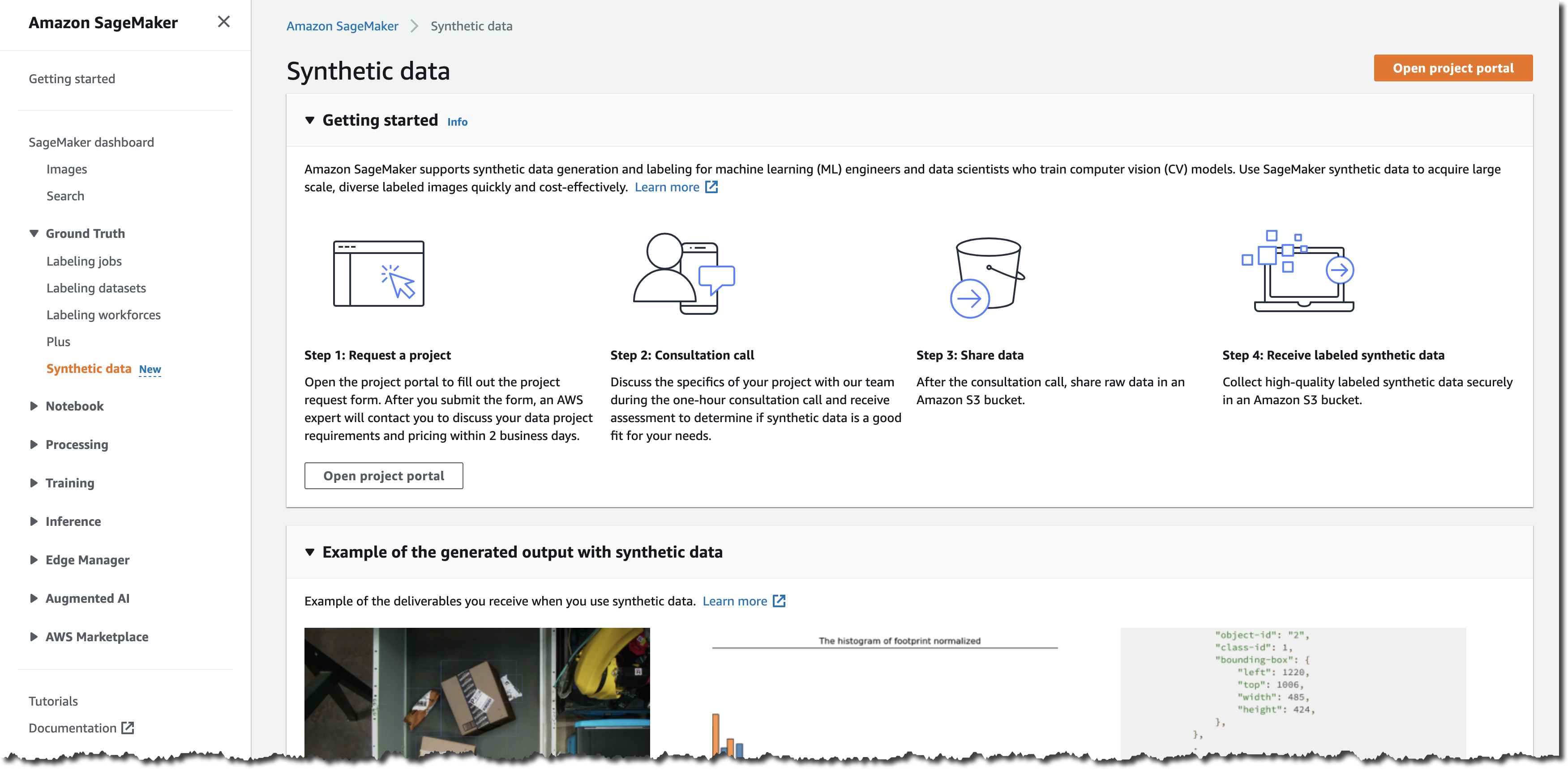
Amazon SageMaker Ground Truth helps you with exactly that. It lets you build highly accurate training datasets for machine learning quickly. SageMaker Ground Truth provides your labelers with built-in workflows and interfaces for common labeling tasks. This process could take several hours or more depending on the size of your unlabeled dataset, and you might have a need to track the progress easily, preferably in the form of a dashboard.

In this blogpost we show how to gain deep insights into the progress of labeling and the performance of the workers by using Amazon Athena and Amazon QuickSight. We use Amazon Athena former to set up several views with specific insights into the labeling progress. Finally we will reference these views in Amazon QuickSight to visualize the data in a dashboard.

This approach also works for combining multiple AWS services in general. AWS provides many building blocks than you can mix-and-match to create a unique, integrated solution with cohesive insights. In this blog post we use data produced by one service (Ground Truth), prepare it with another (Athena) and visualize with a third (QuickSight). The following diagram shows this architecture.

Solution Architecture

ML Solution Architecture

Mapping a JSON structure to a table structure

Ground Truth creates several directories in your Amazon S3 output path. These directories contain the results of your labeling job and other artifacts of the job. The top-level directory for a labeling job has the same name as your labeling job, while the output directories are placed inside it. We will create all insights from what SageMaker Ground Truth calls worker responses.

All respective JSON files reside in the path s3://bucket/<job-name>/annotations/worker-response/.

To analyze the labeling data with Amazon Athena we need to understand the structure of the underlying JSON files. Let’s review the example below. For each item that was labeled, we see the label itself, followed by the submission time and a workerId pointing to an identity. This identity lives in Amazon Cognito, a fully managed service that provides the user directory for our labelers.

{
    "answers": [
        {
            "answerContent": {
                "crowd-classifier": {
                    "label": "Compute"
                }
            },
            "submissionTime": "2020-03-27T10:31:04.210Z",
            "workerId": "private.eu-west-1.1111111111111111",
            "workerMetadata": {
                "identityData": {
                    "identityProviderType": "Cognito",
                    "issuer": "https://cognito-idp.eu-west-1.amazonaws.com/eu-west-1_111111111",
                    "sub": "11111111-1111-1111-1111-111111111111"
                }
            }
        },
        ...
    ]
}

Although the data is stored in Amazon S3 object storage, we are able to use SQL to access the data by using Amazon Athena. Since we now understand the JSON structure from shown in the preceding code, we use Athena and define how to interpret the data that is relevant to us. We do so by first creating a database using the Athena Query Editor:

CREATE DATABASE analyze_labels_db;

Once inside the database, we add the table schema. The actual files remain on Amazon S3, but using the metadata catalog, Athena then knows where the data lies and how to interpret it. The AWS Glue Data Catalog is a central repository to store structural and operational metadata for all your data assets. For a given dataset, you can store its table definition, physical location, add business relevant attributes, in addition to track how this data has changed over time. Besides, Athena the AWS Glue Data Catalog also provides out-of-box integration with Amazon EMR and Amazon Redshift Spectrum. Once you add your table definitions to the Glue Data Catalog, they are available for ETL. They are also readily available for querying in Amazon Athena, Amazon EMR, and Amazon Redshift Spectrum so that you can have a common view of your data between these services.

When going from JSON to SQL, we are crossing format boundaries. To further facilitate how to read the JSON formatted data we are using SerDe Properties to replace the hyphen in crowd-classifier with an underscore due to DDL constraints. Finally we point the location to our Amazon S3 bucket containing the single worker responses. Recognize in the following script that we translate the nested structure of the JSON file itself into a hierarchical, nested data structure in the schema definition. Also, we could leave out the workerMetadata as we don’t need it at this time. The data would still stay in the files on Amazon S3, so that we could later change and add the workerMetadata STRUCT into the table definition for our analysis.

CREATE EXTERNAL TABLE annotations_raw (
  answers array<
    struct<answercontent: 
      struct<crowd_classifier: 
        struct<label: string>
      >,
      submissionTime: string,
      workerId: string,
      workerMetadata: 
        struct<identityData: 
          struct<identityProviderType: string, issuer: string, sub: string>
        >
    >
  >
) 
ROW FORMAT SERDE 'org.openx.data.jsonserde.JsonSerDe'
WITH SERDEPROPERTIES (
  "mapping.crowd_classifier"="crowd-classifier" 
) 
LOCATION 's3://<YOUR_BUCKET>/<JOB_NAME>/annotations/worker-response/'

Creating Views in Athena

Now, we have nested data in our annotations_raw table. For many use cases, especially for analytical uses, representing data in a tabular fashion—as rows—is more natural. This is also the standard way when using SQL and business intelligence tools. To unnest the hierarchical data into flattened rows, we create the following view which will serve as foundation for the other views we create. For an in-depth look into unnesting data with Amazon Athena, read this blog post.

Some of the information we’re interested in might not be part of the document, but is encoded in the path. We use a trick in Athena by using the $path variable from the Presto Hive Connector. This determines which Amazon S3 file contains data that is returned by a specific row in an Athena table. This way we can find out which data object an annotation belongs to. Since Athena is built on top of Presto, we are able to use Presto’s built-in regexp_extract function to find out the iteration as well as the data object id per labeling result. We also cast the submission time in date format to later determine the labeling progress per day.

CREATE OR REPLACE VIEW annotations_view AS
SELECT 
  regexp_extract("$path", 'iteration-[0-9]*') as iteration,
  regexp_extract("$path", '(iteration-[0-9]*\/([0-9]*))',2) as dataRecord,
  answer.answercontent.crowd_classifier.label,
  cast(from_iso8601_timestamp(answer.submissionTime) as timestamp) as submissionTime,
  cast(from_iso8601_timestamp(answer.submissionTime) as date) as submissionDay,
  answer.workerId,
  answer.workerMetadata.identityData.identityProviderType,
  answer.workerMetadata.identityData.issuer,
  answer.workerMetadata.identityData.sub,
  "$path" path
FROM 
  annotations_raw
CROSS JOIN UNNEST(answers) AS t(answer)

This view, annotations_view, will be the starting point for the other views we will be creating in further in this post.

Visualizing with QuickSight

In this section, we explore a way to visualize the views we build in Athena by pointing Amazon QuickSight to the respective view. Amazon QuickSight lets you create and publish interactive dashboards that include ML Insights. Dashboards can then be accessed from any device, and embedded into your applications, portals, and websites.

Thanks to the tight integration between Athena and QuickSight, we are able to map one dataset in QuickSight to one Athena view. In order to further optimize the performance of the dashboard, we can optionally import the datasets into the in-memory optimized calculation engine for Amazon QuickSight called SPICE. With the datasets in place we can now create an analysis in order to interact with the visuals we’re going to add. You can think of an analysis as a container for a set of related visuals. You can use multiple datasets in an analysis, although any given visual can only use one of those datasets. After you create an analysis and an initial visual, you can expand the analysis. You can do this for example by adding datasets and visuals.

Let’s start with our first insight.

Annotations per worker

We’d like to gain insights not only into the total number of labeled items but also on the level of contributions of each individual workers. This could give us an indication whether the labels were created by a diverse crowd of labelers or by a few productive ones. A largely disproportionate amount of contributions from a handful of workers who may have brought along their biases.

SageMaker Ground Truth calls labeled data objects annotations, which is the result of a single workers labeling task.

Luckily we encapsulated all the heavy lifting of format conversion in the annotations_view, so that it is now easy to create a view for the annotations per user:

CREATE OR REPLACE VIEW annotations_per_user AS
SELECT COUNT(sub) AS LabeledItems,
sub AS User
FROM annotations_view
GROUP BY sub
ORDER BY LabeledItems DESC

Next we visualize this view in QuickSight. We add a visual to our analysis, select the respective dataset for the view and use the AutoGraph feature, which chooses the most appropriate visual type. Since we already arranged our view in Athena by the number of labeled items in descending order, there is no need now to sort the data in QuickSight. In the following screenshot, worker c4ef78e4... contributed more labels compared to their peers.

Annotations per worker

This view gives you an indicator to check for a bias that the leading worker might have brought along.

Annotations per label

One thing we want to be aware of is potential imbalances between classes in our dataset. Especially simple machine learning models, which may learn to frequently predict a label that is massively over represented in the dataset. If we can identify an imbalance, we can apply mitigation actions such as upsampling data of underrepresented classes. With the following view we list the total number of annotations per label.

CREATE OR REPLACE VIEW annotations_per_label AS
SELECT Count(dataRecord) AS TotalLabels, label As Label 
FROM annotations_view
GROUP BY label
ORDER BY TotalLabels DESC, Label;

As before, we create a dataset in QuickSight pointing to the annotations_per_label view, open the analysis, add a new visual and leverage the AutoGraph functionality. The result is the following visual representation:

Annotations per worker 2

One can clearly see that the Analytics & AI/ML class is massively underrepresented. At this point, you might want to try getting more data or think about upsampling data for that class.

Annotations per day

Seeing the total number of annotations per label and per worker is good, but we are also interested in how the labeling progress changes over time. This way we might see spikes related to labeller activations. We can also or estimate how long it takes to reach a certain goal of annotations given the current pace. For this purpose we create the following view aggregating the total annotations per day.

CREATE OR REPLACE VIEW annotations_per_day AS
SELECT COUNT(datarecord) AS LabeledItems,
submissionDay
FROM annotations_view
GROUP BY submissionDay
ORDER BY submissionDay, LabeledItems DESC

This time the QuickSight AutoGraph provides us with the following line chart. You might have noticed that the axis labels do not match the column names in Athena. That is because we renamed them in QuickSight for better readability.

Total annotations per day

In the preceding chart we see that there is no consistent pace of labeling, which makes it hard to predict when a certain amount of labeled data will be reached. In this example, after starting strong the progress immediately went down. Knowing this, we might want to take action into motivating our workers to contribute more and validate the effectiveness of these actions with the help of this chart. The spikes indicate an effective short-term action.

Distribution of total annotations by user

We already have insights into annotations per worker, per label and per day. Let us now now see what insights we can get from aggregating some of this information.

The bigger your labeling workforce gets, the harder it can become to see the whole picture. For that reason we will now create a histogram consisting of five buckets. Each bucket represents an interval of total annotations (for example, 0-25 annotations) mapped to the number of users whose amount of total annotations lies in that interval. This allows us to get a sense of what kind of bias might be introduced by the majority of annotations being contributed by a small amount of workers.

To do that, we use the Presto function width_bucket which returns the number of labeled data objects according to the five buckets we defined with a size of 25 each. We define these buckets by creating an Array with 5 elements that specify the boundaries.

CREATE OR REPLACE VIEW users_per_bucket_annotations AS
SELECT 
bucket,numberOfUsers,
CASE
   WHEN bucket=5 THEN 'B' || cast(bucket AS VARCHAR(10)) || ': ' || cast(((bucket-1) * 25) AS VARCHAR(10)) || '+'
   ELSE 'B' || cast(bucket AS VARCHAR(10)) || ': ' || cast(((bucket-1) * 25) AS VARCHAR(10)) || '-' || cast((bucket * 25) AS VARCHAR(10))
END AS NumberOfAnnotations
FROM
(SELECT width_bucket(labeleditems,ARRAY[0,25,50,75,100]) AS bucket,
 count(user) AS numberOfUsers
FROM annotations_per_user
GROUP BY 1
ORDER BY bucket)

A SELECT * FROM users_per_bucket_annotations produces the following result:

A SELECT FROM users_per_bucket_annotations

Let’s now investigate the same data via QuickSight:

Annotations per User in buckets of Size 25

Now that we can look at the data visually it becomes clear that we have a bimodal distribution, with many labelers having done very little, and many labelers doing quite a lot. This may warrant interviewing some labelers to find out if there is something holding back users from progressing, or if we can keep engagement high over time.

Putting it all together in QuickSight

Since we created all previous visuals into one analysis, we can now utilize it as a central place to consume our insights in a user-friendly way. Moreover, we can share our insights with others as a read-only snapshot which QuickSight calls a dashboard. User who are dashboard viewers can view and filter the dashboard data as below:

Groundtruth dashboard

Furthermore, you can generate a report and let QuickSight send it either once or on a schedule (daily, weekly or monthly) to your peers. This way users do not have to sign in and they can get reminders to check the progress of the labeling job. Lastly, sending out those reports is an opportunity to stay in touch with the labelers and keep the engagement high.

Conclusion

In this blogpost, we have shown one example of combining multiple AWS services in order to build a solution tailored to your needs. We took the Amazon S3 output generated by SageMaker Ground Truth and showed how it can be further processed and analyzed with Athena. Finally, we created a central place to consume our insights in a user-friendly way with QuickSight. By putting it all together in a dashboard we were able to share our insights with our peers.

You can take the same pattern and apply it to other situations: take some of the many building blocks AWS provides and mix-and-match them to create a unique, integrated solution with cohesive insights just as we did with Ground Truth, Athena, and QuickSight.

Field Notes provides hands-on technical guidance from AWS Solutions Architects, consultants, and technical account managers, based on their experiences in the field solving real-world business problems for customers.