All posts by Anubhav Awasthi

A systematic approach to benchmarking SQL processing engines on AWS

2026-05-19 Anubhav Awasthi

Post Syndicated from Anubhav Awasthi original https://aws.amazon.com/blogs/big-data/a-systematic-approach-to-benchmarking-sql-processing-engines-on-aws/

Selecting the right SQL processing solution for large-scale data analytics is a critical decision for organizations. As data volumes grow exponentially, the technology landscape has evolved to offer diverse options for processing and analyzing this information efficiently. This post presents a systematic framework for evaluating and benchmarking SQL processing engines on AWS, using Apache JMeter to conduct practical performance testing at scale.

The AWS analytics ecosystem

AWS offers a rich portfolio of SQL processing solutions to meet various analytical needs:

Serverless query services – Amazon Athena is a serverless, interactive query service that uses standard SQL to analyze data in Amazon Simple Storage Service (Amazon S3), offering automatic scaling, parallel query execution, and pay-per-query pricing with no infrastructure management required
Data warehouse solutions – Amazon Redshift offers scalable, high-performance cloud data warehousing with serverless options, zero-ETL integrations, AI-powered query assistance, and seamless machine learning (ML) integration for modern analytics at scale
Managed open source engines – Amazon EMR supports Apache Spark SQL, Apache Trino (formerly PrestoSQL), and other distributed query frameworks
Self-managed options – You can deploy open source engines like Apache Spark, Apache Flink, and Trino on Amazon Elastic Kubernetes Service (Amazon EKS) for greater control
Partner solutions – You can access specialized big data analytics tools through AWS Marketplace

These options are further enhanced by modern open table formats such as Apache Iceberg, Delta Lake, and Apache Hudi, which bring crucial enterprise features like ACID (Atomicity, Consistency, Isolation, and Durability) transactions, schema evolution, and time travel capabilities to data lakes. These SQL processing solutions operate under the AWS Shared Responsibility Model. AWS manages the security of the underlying infrastructure and services, and customers are responsible for secure configuration, access management, and data protection within their testing environments. This division of responsibility remains important when evaluating and benchmarking different SQL engines. Proper security configuration and implementation by customers is essential for maintaining a secure analytics environment.

Evaluation challenges in SQL engine selection

The rich ecosystem of SQL processing options creates significant evaluation challenges. Each SQL engine employs unique architectural approaches and optimization strategies, making direct comparisons complex. Organizations embarking on this evaluation journey face several interconnected obstacles:

Creating environments that accurately reflect production scenarios
Developing test datasets that mirror real-world data characteristics and volumes
Replicating real-world query patterns and concurrency levels
Maintaining uniform testing conditions across different engine architectures
Controlling infrastructure expenses throughout the evaluation process

Performance considerations at petabyte scale

When evaluating solutions for petabyte-scale deployments, the complexity intensifies considerably. Several critical factors come into play:

Resource management – Distributed SQL engines require precise balancing of CPU, memory, and storage resources. Suboptimal resource allocation can lead to query failures and performance degradation, particularly as data volumes grow.
Data distribution patterns – How data is distributed across partitions or nodes significantly impacts query performance. Data skew can create processing bottlenecks, with some nodes handling disproportionate workloads while others remain underutilized.
Concurrency handling – High-concurrency environments demand sophisticated workload scheduling and resource isolation mechanisms. The ability to maintain consistent performance under varying concurrent loads becomes a critical differentiator between solutions.
Meaningful metrics – Performance evaluation at scale requires comprehensive metrics analysis:
- Mean, median, and percentile response times (particularly p90 and p95)
- Query throughput under varying concurrency levels
- Scalability characteristics across diverse workload types
- Resource utilization efficiency during peak loads

Limitations of traditional benchmarks

Although industry-standard benchmarks like TPC-DS and TPC-H provide valuable insights, our experience with multiple customer engagements has shown that tailored, workload-specific testing often reveals performance characteristics not captured by these standardized tests. This is especially true for complex, multi-tenant environments with diverse query patterns. Organizations that complement standard benchmarks with workload-specific testing typically experience shorter proof-of-concept cycles, optimized evaluation costs, and more efficient testing operations. This comprehensive approach helps reduce uncertainty in the final solution selection process.

Prerequisites

Before you dive into the evaluation process, make sure you have the following prerequisites:

An AWS account with appropriate permissions to create and manage Amazon Elastic Compute Cloud (Amazon EC2) instances and access the SQL engines you plan to benchmark.
Basic familiarity with AWS services, particularly Amazon EC2 and the SQL engines you intend to evaluate (such as Athena, Amazon Redshift, or Amazon EMR).
Experience with SQL and data analytics concepts.
Access to the SQL engines you choose to benchmark. This post assumes you’ve already set up the engines you want to test. For setup instructions, refer to the AWS documentation for each service.
A dataset suitable for your benchmarking needs. Dataset creation and loading are not covered in this post. Build petabyte-scale synthetic test data with Amazon EMR on EC2 provides prescriptive guidance to generate test datasets at scale. Make sure your test datasets are stored in S3 buckets with encryption enabled (using SSE-KMS or SSE-S3) and that all service connections use TLS for data in transit.

Benefits of Apache JMeter

As organizations scale their analytics workloads to petabyte levels, there is a growing need for a robust, structured approach to SQL query performance testing. Although many organizations develop custom testing frameworks or use various benchmarking tools, these approaches often lack standardization and can be difficult to replicate across different SQL engines. The complexity of modern data architectures, combined with the variety of available SQL processing solutions, demands a systematic evaluation methodology. Apache JMeter emerges as a powerful solution to address this challenge. Though traditionally known for web application testing, JMeter’s extensible architecture and robust feature set make it particularly well-suited for SQL performance testing at scale.JMeter offers several advantages for evaluating SQL engines:

Support for multiple protocols and connections
Ability to simulate complex concurrent workloads
Built-in performance metrics and reporting
Extensible architecture for custom testing scenarios
Integration capabilities with continuous integration and continuous delivery (CI/CD) pipelines

Through this proposed framework, which has been validated across multiple customer engagements at petabyte scale, we aim to help organizations make more informed decisions when selecting a SQL processing solution. Our experience working with customers to assess various AWS Analytics services and open source solutions has demonstrated that a systematic evaluation approach significantly reduces proof-of-concept cycles and optimizes resource investments. This framework has helped organizations effectively evaluate services like Athena, Amazon Redshift, and Amazon EMR, alongside open source solutions such as Trino on Amazon EKS, based on their specific workload profiles and performance requirements.With this methodology, organizations can accomplish the following:

Navigate the complex landscape of large-scale data processing technologies
Reduce proof-of-concept cycles from months to weeks
Minimize infrastructure costs during evaluation phases
Make data-driven decisions about technology selection
Better align technology choices with business requirements
Establish repeatable testing patterns for future evaluations

Testing methodology in practice

A successful SQL engine evaluation requires understanding and replicating real-world workload patterns. Our methodology, refined through numerous customer engagements, focuses on comprehensive testing across multiple dimensions while remaining adaptable to specific organizational needs.

Query pattern selection

We begin by selecting representative query patterns that mirror production workloads:

Aggregation queries that summarize large datasets using operations like SUM, AVG, and COUNT
Complex join operations that test the engine’s ability to combine data efficiently across multiple tables
String operations that evaluate text processing capabilities
Nested queries that assess the engine’s optimization capabilities for complex query structures

A carefully selected set of 8–10 queries typically provides sufficient coverage while keeping the evaluation manageable. These should reflect your actual workload characteristics and business requirements.

Data volume variations

Testing across different data volumes is important for understanding scalability characteristics. We structure our tests around varying data scan ranges:

Small-scale scans – Queries accessing 1–7 days of data (megabytes to gigabytes)
Large-scale scans – Queries spanning 14–30 days (terabytes to petabytes)

This approach evaluates both I/O efficiency with large datasets and metadata handling with smaller, frequent queries, helping understand how services like Amazon EMR, Amazon Redshift, or Athena optimize query execution across different access patterns.

Concurrency testing

Real-world analytics environments rarely process single queries in isolation. Our methodology incorporates the following features:

Progressive concurrency testing starting at lower levels (typically 16, 32, 64, and 128 parallel queries), though these numbers can be adjusted based on your test infrastructure capacity and specific requirements. We recommend starting with smaller concurrency levels and gradually scaling up to understand performance characteristics
Varied query complexity and frequency (referred to as query weights) to simulate realistic workload distributions. This means some queries are run more often or are more resource-intensive than others, mimicking real-world usage patterns.
Mixed query patterns running simultaneously to test resource management.
Consistent execution across different date ranges to evaluate scaling behavior.

This approach is particularly important when evaluating managed services like the workload management capabilities of Amazon Redshift or the resource allocation strategies of Amazon EMR.

Query weight distribution

Production environments typically see varying frequencies of different query types. Our framework incorporates weighted query distribution to simulate real-world scenarios more accurately. In a typical distribution, frequent lightweight queries might represent 60% of the workload, complex analytical queries might comprise 30%, and resource-intensive data processing operations might make up the remaining 10%.This weighted approach makes sure performance testing reflects actual usage patterns rather than artificial benchmarking scenarios. The exact distribution should mirror your organization’s specific workload patterns.

Sequential vs. concurrent testing

Our methodology implements two distinct testing phases:

Sequential testing – Establishes baseline performance metrics:
- Runs each query type independently across different date ranges
- Runs multiple iterations to provide consistency and identify variability
- Helps understand individual query performance characteristics
Concurrent testing – Simulates real-world multi-user scenarios:
- Implements weighted query distributions
- Tests different concurrency levels to identify scaling limitations
- Evaluates resource management capabilities of different engines

JMeter efficiently implements both testing phases while maintaining consistent test conditions across SQL engines. Its ability to handle various JDBC connections makes it particularly suitable for testing AWS analytics services.Through this structured approach, organizations can gather comprehensive performance data reflecting their specific use cases, enabling informed SQL engine selection decisions while maintaining core principles of systematic evaluation and realistic workload simulation.

Test plans

To evaluate SQL engines’ performance under varying workloads, we designed two test scenarios: sequential and concurrent execution plans. Each scenario was executed across different data volumes by adjusting the query date range filters to cover 1, 7, 14, and 30 days. These variations simulate typical analytical workloads with progressively increasing data sizes.For sequential runs, each test was treated as a distinct batch, grouping all queries (Query 1 to Query 9) under the same date range—each query will scan data for 1, 7, 14, and 30 days with appropriate date filtering in the query’s where predicate. We used JMeter to capture average query response times for each batch. This configuration was run three times, and the final metrics reflect the average response time across these iterations to ensure reliability and account for environmental variance.Although three iterations provide initial insights, if you observe significant variations in results (typically more than 10% deviation between runs), consider expanding to 10 or more iterations. This additional sampling helps establish statistical significance, identify true performance patterns, and distinguish outliers (beyond three standard deviations) from normal variations. Document any consistent anomalies, because they may indicate important performance or security considerations for your specific environment.The following table shows the sample test plans template for the sequential test plan run.

Dataset Time Range	Run	Query Weights
Dataset Time Range	Run	Query 1	Query 2	Query 3	Query 4	Query 5	Query 6	Query 7	Query 8	Query 9
1 day	Run 1
	Run 2
	Run 3
	Avg
7 days	Run 1
	Run 2
	Run 3
	Avg
14 days	Run 1
	Run 2
	Run 3
	Avg
30 days	Run 1
	Run 2
	Run 3
	Avg

For the concurrent test plan, we introduced a probabilistic weighted distribution to the queries (Query 1 to Query 9), simulating a more realistic production-like environment where query frequency varies based on business relevance and usage patterns. This added a layer of complexity to better reflect how the SQL engine would perform under real-world concurrent access patterns.The following table shows the sample test plans template for the concurrent test plan run.

Dataset Time Range	Concurrent Runs	Query Weights
Dataset Time Range	Concurrent Runs	Query 1	Query 2	Query 3	Query 4	Query 5	Query 6	Query 7	Query 8	Query 9
1 days	8	11%	11%	11%	11%	11%	11%	11%	11%	11%
	16	10%	5%	24%	5%	5%	5%	24%	14%	10%
	32	8%	3%	24%	5%	5%	5%	24%	16%	8%
	64	7%	3%	24%	6%	4%	6%	26%	16%	9%
	128	1%	4%	19%	8%	5%	7%	14%	20%	22%
*7 days	8	11%	11%	11%	11%	11%	11%	11%	11%	11%
	16	10%	5%	24%	5%	5%	5%	24%	14%	10%
	32	8%	3%	24%	5%	5%	5%	24%	16%	8%
	64	7%	3%	24%	6%	4%	6%	26%	16%	9%
	**128	1%	4%	19%	8%	5%	7%	14%	20%	22%
14 days	8	11%	11%	11%	11%	11%	11%	11%	11%	11%
	16	10%	5%	24%	5%	5%	5%	24%	14%	10%
	32	8%	3%	24%	5%	5%	5%	24%	16%	8%
	64	7%	3%	24%	6%	4%	6%	26%	16%	9%
	128	1%	4%	19%	8%	5%	7%	14%	20%	22%
30 days	8	11%	11%	11%	11%	11%	11%	11%	11%	11%
	16	10%	5%	24%	5%	5%	5%	24%	14%	10%
	32	8%	3%	24%	5%	5%	5%	24%	16%	8%
	64	7%	3%	24%	6%	4%	6%	26%	16%	9%
	128	1%	4%	19%	8%	5%	7%	14%	20%	22%

For example, for configuration of *7 days concurrent run with **128 concurrency, the proposed configuration distributes Query 1 to Query 9 with appropriate weighted submissions such that Query 9 is executed the greatest number of times in the overall 128 executions submitted across all 9 queries for this run.

JMeter setup

To begin, you must set up JMeter on a machine that can handle the desired test load. An EC2 instance is a flexible and cost-effective option. Choose an instance type with sufficient vCPUs to support your maximum planned concurrency. For example, a c6i.4xlarge or higher is typically suitable for moderate to high throughput testing scenarios. For the operating system, you might choose Amazon Linux, which is optimized for AWS. For production-grade testing environments, deploy the JMeter EC2 instance in a private subnet of a virtual private cloud (VPC) with appropriate security groups that allow only required connections. This network isolation helps maintain security while executing performance tests. Consider using Amazon Virtual Private Cloud (Amazon VPC) endpoints for secure access to AWS services.

After the instance is provisioned, install Java (Java 17 LTS or Java 21 LTS) and download the latest version of JMeter. Be sure to configure the system with appropriate JVM options to allocate sufficient heap memory for large-scale test executions. Refer to Getting Started to learn more.

# Install Java
sudo yum update -y # For Amazon Linux
sudo yum install java-17-amazon-corretto -y

# Download JMeter and place the appropriate jdbc driver for the engine of your selection under lib folder
wget https://downloads.apache.org//jmeter/binaries/apache-jmeter-5.6.3.tgz
tar -xvzf apache-jmeter-5.6.3.tgz
cd apache-jmeter-5.6.3/lib

# Launch JMeter in GUI mode (if using a GUI-capable setup) or use CLI for remote testing
./bin/jmeter

JMeter concepts

Before you create test plans in JMeter, it’s important to understand a few foundational concepts that influence how your test plan behaves—such as thread groups, user-defined variables, and JDBC connection. These components enable the simulation of real-world query loads, including concurrency and pacing.

Test plans

The test plan is the top-level container for a JMeter test. It defines the overall testing strategy, including the queries to execute, their parameters, and the concurrent user behavior. These plans are represented as jmx files that can then be used for CLI-based execution. JMeter supports both GUI and CLI modes. It is highly recommended that you use the JMeter GUI primarily for creating test plans as jmx, and use the CLI for large load tests. You can also run thread groups consecutively for sequential execution. The default behavior is to run all thread groups in parallel suited for concurrent execution. Refer to Building a Test Plan to learn more about options available with test plans.

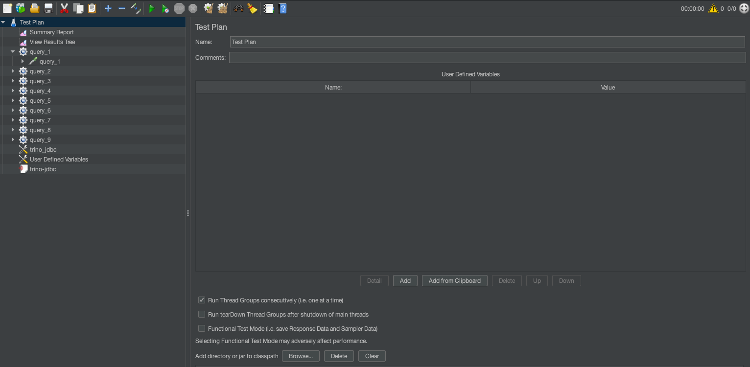
User-defined variables

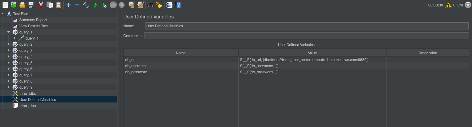
User-defined variables are global parameters that you can reuse throughout the test plan. They are helpful for defining database credentials, server URLs, or query parameters. For example:DB_URL=jdbc:trino://trino-cluster.example.com:8889?SSL=true #Enable SSL/TLS

You can configure authentication (user name and password) through your organization’s approved methods, such as AWS Secrets Manager (see Move hardcoded secrets to AWS Secrets Manager) AWS Identity and Access Management (IAM) roles, or other secure credential management systems.

Thread groups

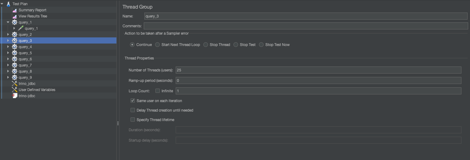
A thread group represents a group of virtual users (threads) executing test actions. Each thread simulates a single user sending requests to the SQL engine. This can be used to simulate concurrent runs. For example, in the preceding template, Query 3 has 19% weightage across 128 runs. This means .19*128=25 total runs, so we set the thread group to 25.

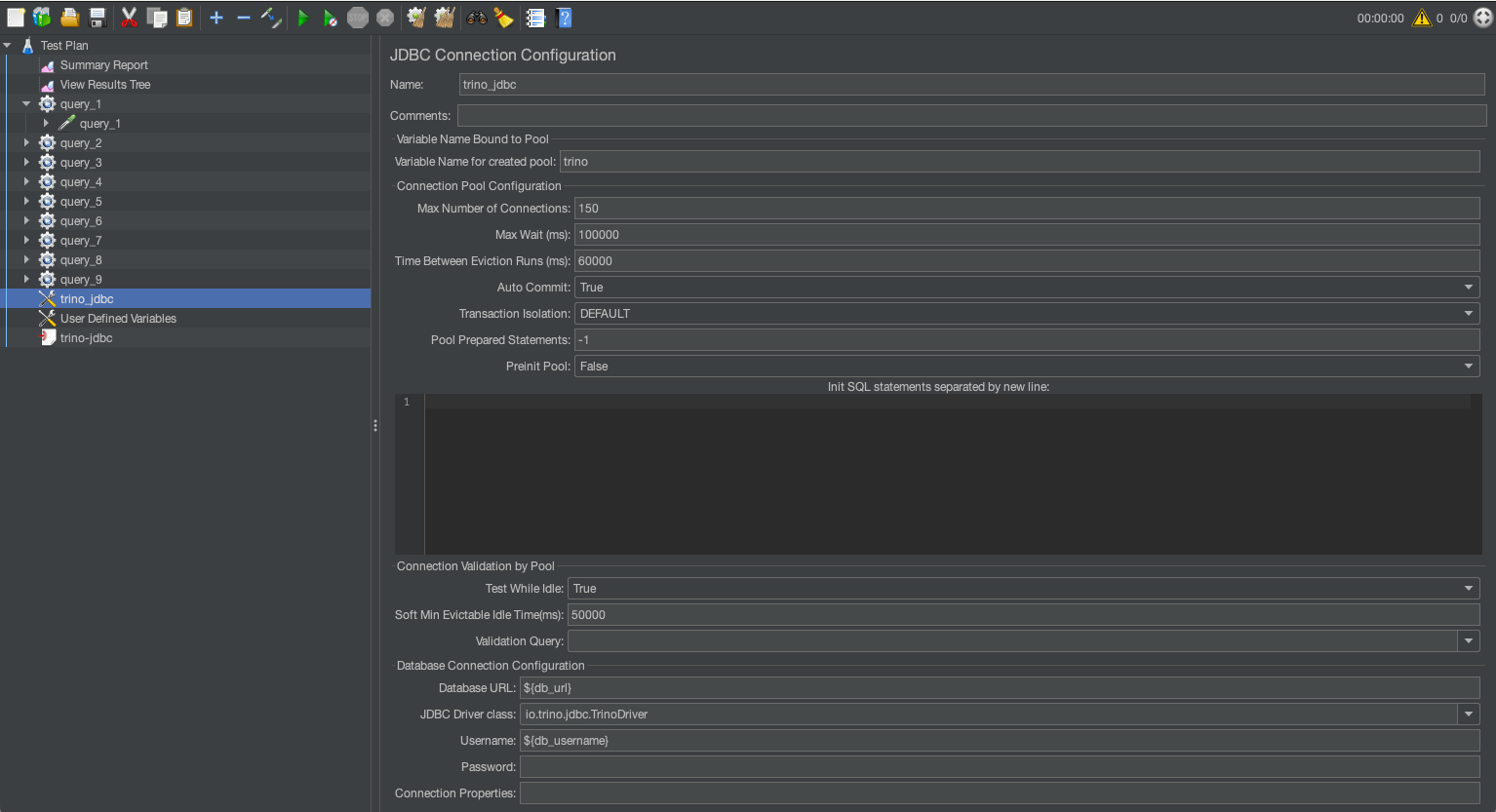
JDBC connection configuration

JDBC connection configuration sets up the database connection for the test. It specifies the database URL, driver, and credentials required for executing SQL queries. Key fields to configure are database URL and JDBC driver class. The following table summarizes the different configuration settings.

SQL Engine	JDBC Driver	JDBC Driver Class
Trino on EMR	`trino-jdbc-<trino_version>-amzn-0.jar`	`io.trino.jdbc.TrinoDriver`
Athena	Athena JDBC 3.x driver	`com.amazon.athena.jdbc.AthenaDriver`
Amazon Redshift	Amazon Redshift JDBC driver	`com.amazon.redshift.jdbc.Driver`
Trino on EKS	Trino JDBC driver	`io.trino.jdbc.TrinoDriver`

JDBC requests

The JDBC request executes SQL queries against the database using the configuration defined in the JDBC connection configuration.

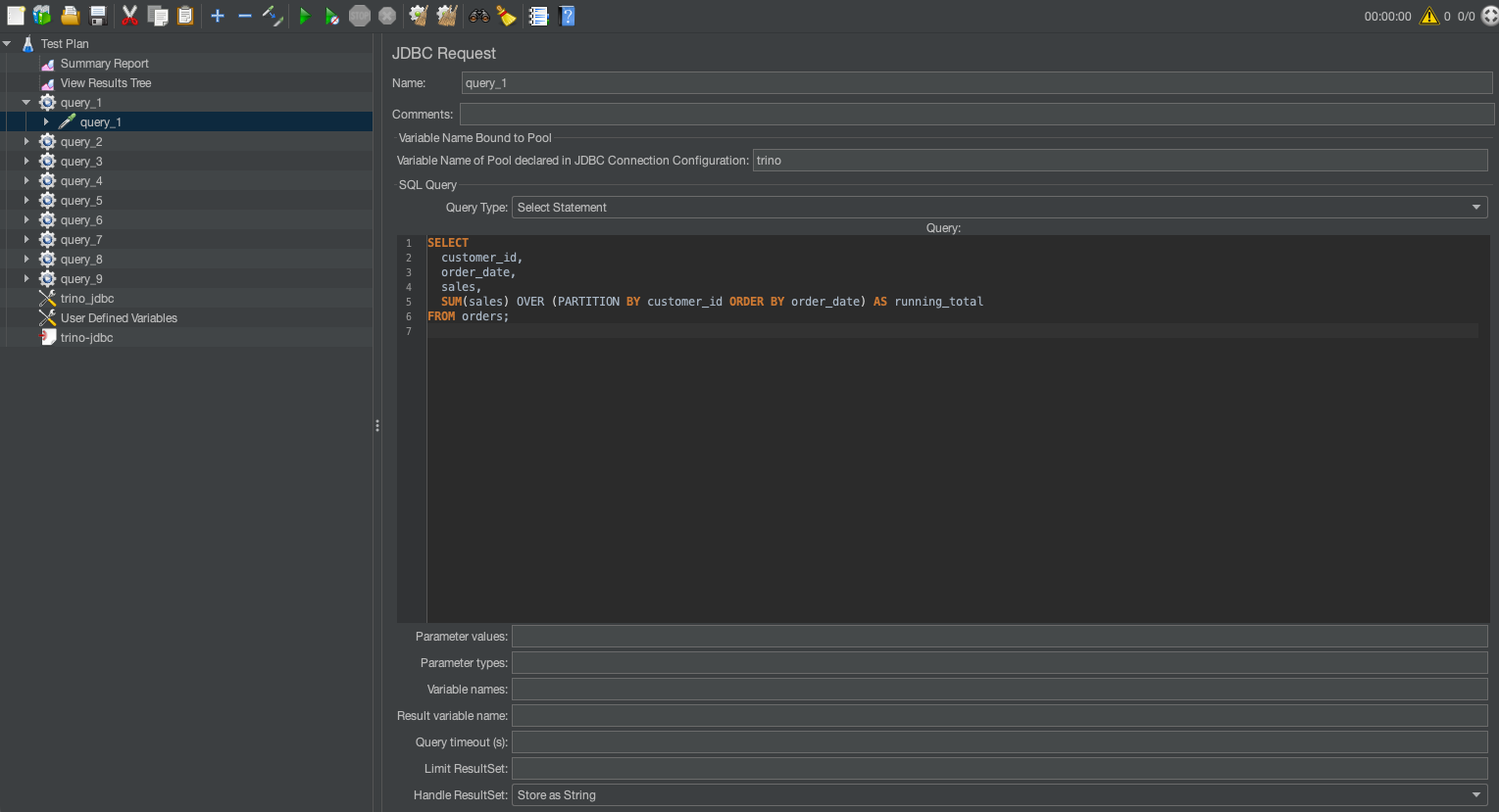
For example, following command runs the JMeter in CLI mode:

# Run benchmarks in CLI mode 
./jmeter -n -t <path_to>.jmx -l <local path for log>.log -e -o <local path for>/output/

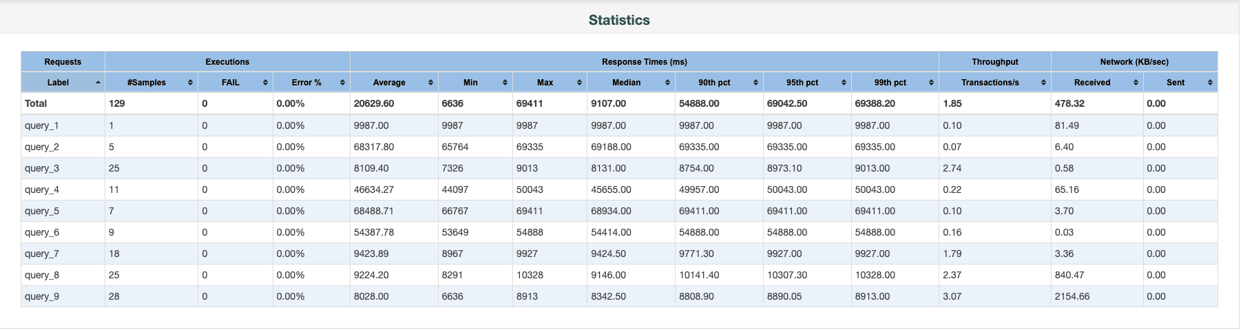
The output folder will contain an HTML report with different statistics. The following screenshot illustrates 128 concurrent runs.

Monitoring and logging

For comprehensive visibility and audit requirements, enable AWS CloudTrail logging, VPC Flow Logs, and service-specific logs (like Amazon S3 access logs). These logs can be centralized in Amazon CloudWatch Logs for monitoring and analysis. This provides proper audit trails while evaluating different SQL engines and helps track access patterns and potential security events.

Post-test steps

After running your JMeter tests, proceed with the following steps:

Review the HTML report’s key metrics, including response times, throughput, and error rates across different query types and concurrency levels.
Run identical test plans across your candidate SQL engines for direct performance comparison.
Refine your test plans based on initial findings, focusing on areas where performance differences are significant.
Factor in the cost implications alongside performance metrics to make a balanced decision.

These steps can help you systematically evaluate and select the most suitable SQL engine for your analytics workloads.

Resources

In the preceding steps, we walked through a UI-based setup for JMeter along with test plans. We have created a few sample JMeter test plans for both sequential and concurrent runs along with sample test reports. You can modify the plans to fit your needs.

JMeter sample report
JMeter test plan for sequential run
JMeter test plan for concurrent run

Clean up

After you complete your benchmarking process, clean up the resources to avoid unnecessary costs:

Stop or delete the EC2 instances used for running JMeter.
Depending on which SQL engines you used for testing, clean up active resources.
Review your AWS Management Console to confirm no active resources remain.
If you created test datasets in Amazon S3 or other storage services specifically for this benchmarking, consider deleting them if they’re no longer needed.
Although JMeter test plans and results don’t incur AWS costs, organize or delete local files as needed for your record-keeping.

Summary

Selecting the right SQL processing solution for large-scale analytics demands a systematic, data-driven approach. Our JMeter framework can help organizations effectively evaluate different SQL engines by simulating real-world workload patterns across various query types, data volumes, and concurrency levels. This methodology reduces proof-of-concept cycles and provides insights beyond traditional benchmarks, helping you assess managed AWS services like Athena and Amazon Redshift and open source solutions on Amazon EKS.

About the authors

Build petabyte-scale synthetic test data with Amazon EMR on EC2

2026-05-19 Anubhav Awasthi

Post Syndicated from Anubhav Awasthi original https://aws.amazon.com/blogs/big-data/build-petabyte-scale-synthetic-test-data-with-amazon-emr-on-ec2/

As you scale your data systems, you face a challenge: how to test thoroughly without putting customer data at risk. Using production data for testing can expose sensitive customer information to unauthorized access or breaches. For customers in regulated industries like finance and healthcare, this risk isn’t only a concern. It’s unacceptable. A data breach during testing could compromise their privacy, damage their trust, and expose organizations to significant compliance penalties. Synthetic test data solves this problem by generating artificial datasets that replicate the structure and patterns of real data without containing any actual customer information. This approach means you can test performance, validate data pipelines, and develop new features while ensuring that customer data remains protected and compliance requirements are met.

As data volumes grow from terabytes to petabytes, the architecture for generating synthetic data must evolve to meet increasing demands for scale, performance, and data quality. In this post, we show how you can build a scalable synthetic data generation solution using Amazon EMR, Apache Spark, and the Faker library.

The challenge of synthetic data generation

Traditional benchmark datasets like TPC-DS provide standardized schemas and predetermined data volumes for consistent testing environments across different systems. However, they fall short in meeting real-world testing requirements. These benchmarks don’t capture industry-specific patterns or the complex relationships found in actual production data. Their rigid schemas and simplified distributions fail to reflect business requirements, and scaling them while maintaining data consistency proves difficult. Perhaps most critically, generating massive datasets with traditional approaches requires specialized architectures to avoid proportional increases in compute costs and time.

Requirements for production-grade synthetic data

Effective workload validation demands synthetic data that mirrors production distributions while maintaining referential integrity across related tables and entities. The generation process must scale horizontally to accommodate growing data volumes while delivering deterministic results. Given identical input parameters, the system should produce the same dataset across multiple runs, supporting consistent testing cycles and comparative analysis.

Beyond technical requirements, synthetic data addresses compliance needs by minimizing exposure of personally identifiable information (PII) and protected health information (PHI) in non-production environments. This approach satisfies GDPR, HIPAA, and CCPA requirements while supporting secure cross-border data transfer, regular stress testing without compromising sensitive information, and providing an audit-friendly alternative to data masking that preserves analytical properties.

Solution overview

Architecting a synthetic data generation system that scales from terabytes to petabytes requires balancing several competing demands: the system must scale horizontally while maintaining data quality, generate large volumes efficiently, manage compute and storage resources cost-effectively, and support various schemas and output formats.

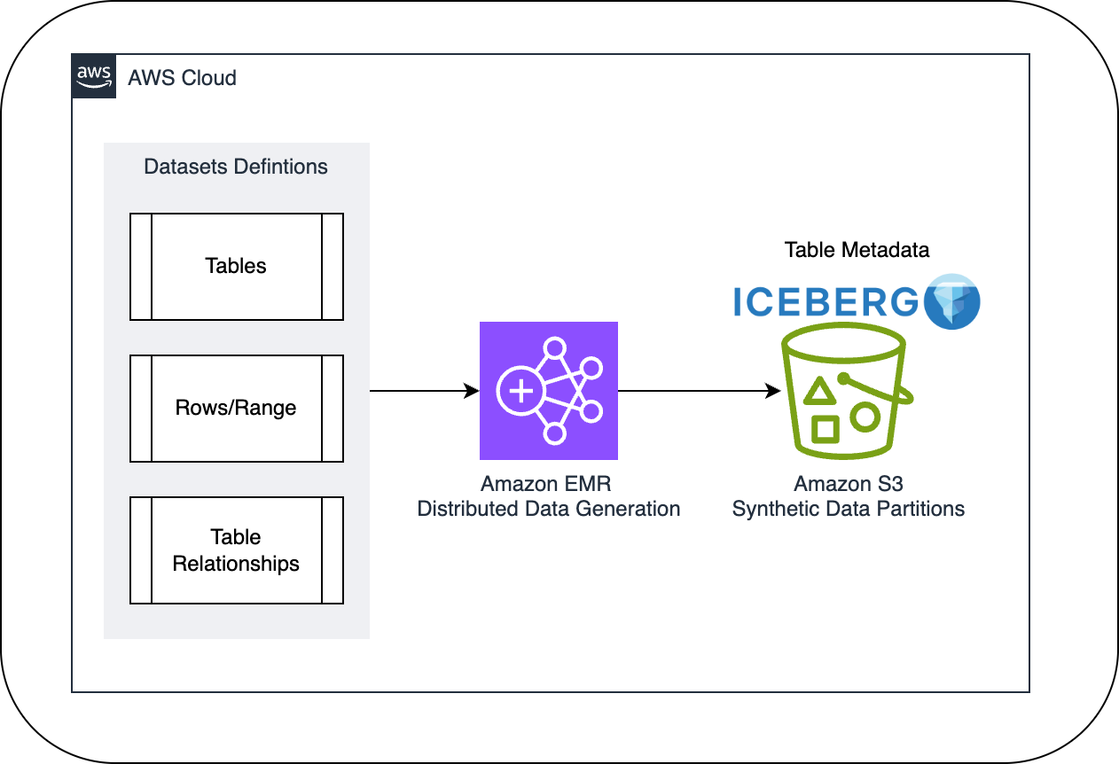
Our architecture addresses these challenges through four core components. Apache Spark on Amazon EMR provides the distributed computing framework necessary for large-scale generation. The Faker library offers synthetic data generation functions that integrate with Spark. Amazon Simple Storage Service (Amazon S3) with Apache Iceberg serves as the storage layer. We chose Iceberg for its schema and partition evolution capabilities without data rewrites, atomic transactions for consistency, precise time travel features for reproducible testing, and optimized performance at extreme scale. Amazon EMR handles dynamic resource allocation and cluster management.

The following diagram illustrates the solution architecture.

Solution architecture showing Amazon EMR generating synthetic data with Apache Spark and Faker, storing results in Amazon S3 with Apache Iceberg

Synthetic data generation at scale with Amazon EMR

Amazon EMR emerges as a particularly powerful solution for this use case, offering several advantages that directly address our requirements. It facilitates scaling of compute resources through instance fleets and Spot Instances, which can reduce costs by up to 90% compared to On-Demand pricing. The service provides built-in performance optimization for Spark applications with real-time monitoring through Amazon CloudWatch integration.

The managed infrastructure reduces operational overhead by handling the underlying Spark ecosystem and cluster lifecycle, while still providing control over scaling policies, instance types, and configurations. Integration with Amazon S3, AWS Glue, and Amazon Athena facilitates end-to-end data generation and testing workflows. Support for multiple programming languages and notebooks provides flexibility in implementing generation logic tailored to specific testing scenarios.

The synthetic data generation process follows a systematic approach designed for efficiency and scalability, as illustrated in the following diagram.

Synthetic data generation workflow showing the systematic process from configuration through data generation to storage

Although synthetic data generation isn’t a sensitive workload, it’s important to maintain robust security throughout the data generation process. Amazon EMR provides security features that align with organizational compliance requirements.

For comprehensive security guidance specific to Amazon EMR deployments, refer to Security in Amazon EMR. The solution follows the AWS Shared Responsibility Model, where AWS manages the security of the cloud infrastructure, and customers maintain responsibility for data security, access management, and compliance controls in the cloud. Specifically for synthetic data generation workloads, AWS manages the security of the underlying Amazon EMR infrastructure, network, and service operations, and customers implement appropriate security controls for their data generation pipelines. Consider the following key areas:

Data protection – Enable encryption at rest and in transit using Amazon EMR security configurations, including Amazon S3 encryption and TLS certificates for inter-node communication.
Network security – Deploy Amazon EMR clusters in private subnets with security groups following least privilege, and enable the Amazon EMR block public access feature.
Access control – Implement AWS Identity and Access Management (IAM) roles with least privilege for Amazon EMR service roles, Amazon Elastic Compute Cloud (Amazon EC2) instance profiles, and runtime roles to isolate job access. Fine-grained table-level and column-level permissions can be controlled using AWS Lake Formation. Additional authentication options are available using Kerberos and LDAP.

Optimize Faker for petabyte-scale data generation

When generating synthetic data at petabyte scale, using Faker’s implementations can quickly lead to performance bottlenecks. To overcome these limitations, adopt a combination of different optimization approaches instead of the default setup. Some of the approaches we adopted in this scenario are discussed in this section.

Faker instance pooling

The following code creates multiple Faker instances to avoid contention when generating data in parallel:

NUM_FAKER_INSTANCES = 10
faker_pool = [Faker() for _ in range(NUM_FAKER_INSTANCES)]

Consistent seed management

The following code provides reproducible data generation across distributed executors:

for faker in faker_pool:
    faker.seed_instance(42)  # For reproducibility
    random.seed(42)

Random access to Faker pool

The following code distributes load across multiple Faker instances to reduce contention:

faker = faker_pool[random.randint(0, NUM_FAKER_INSTANCES-1)]

Broadcast variables for reference data

The following code efficiently distributes reference data to all executors:

tenant_ids_broadcast = spark.sparkContext.broadcast(tenant_ids)
protocols_bc = spark.sparkContext.broadcast(protocols)

Batch generation of synthetic data

The following code generates fake data in batches rather than one-by-one:

return spark.range(1, num_endpoints + 1)
    .withColumn("hostname", random_hostname_udf())

ThreadPoolExecutor for parallel processing

The following code uses Python’s threading for parallel operations within executors:

def parallel_write_with_sync(dataframe_configs, max_workers=3):
    with ThreadPoolExecutor(max_workers=max_workers) as executor:
        # Parallel processing

Optimize Amazon EMR and Spark

When processing massive datasets with Spark on Amazon EMR, carefully tuning configurations can substantially enhance performance beyond the standard settings. In this section, we discuss ways to optimize the execution environment, so you can efficiently handle petabyte-scale workloads with synthetic data generation. By strategically using Spark’s advanced features and configuring Amazon EMR for your specific use case, you can improve throughput, reduce processing time, and maximize resource utilization.

Arrow configuration

The following code enables Apache Arrow for efficient data transfer between Python and JVM. The default value is false.

.config("spark.sql.execution.arrow.pyspark.enabled", "true")

Enable this configuration when your PySpark application frequently converts data between Python and JVM, especially for large DataFrames or when using Pandas operations. Keep this setting disabled for pure Spark SQL workloads or when memory is constrained.

This optimization is most effective in the following scenarios:

When processing large-scale datasets that require frequent conversion between Python and JVM.
In a PySpark application where large DataFrame operations and Pandas integration are needed.
With data science workloads that combine Python UDFs with Spark SQL operations.

Consider the following trade-offs:

Arrow maintains in-memory columnar format, resulting in increased memory consumption.
Not all data types are fully supported in older versions of Spark.
It might introduce overhead for very small datasets where conversion costs outweigh the benefits.

Adaptive query execution

The following code allows Spark to dynamically optimize query execution plans. The default value is true in Spark 3.2 and later, and false in earlier versions.

.config("spark.sql.adaptive.enabled", "true")

This optimization is generally recommended to keep enabled for most workloads. Consider disabling only when you have highly optimized, predictable queries where the adaptive overhead isn’t beneficial, or when troubleshooting query performance issues.

This optimization is most effective in the following scenarios:

Complex join operations with unknown or skewed data distributions.
Multi-stage queries where initial plans might be suboptimal.
When processing data with changing characteristics over time.

Consider the following trade-offs:

You may experience additional overhead during the query planning phase.
You might occasionally choose suboptimal plans for certain edge cases.

Parallelism configuration

The following code sets appropriate parallelism for distributed data processing based on the volume of data you’re generating. The default value for spark.default.parallelism is the total number of cores on all executor nodes or 2, whichever larger. The default value for spark.sql.shuffle.partitions is 200.

.config("spark.default.parallelism", 1000)
.config("spark.sql.shuffle.partitions", 1000)

Adjust this configuration when the default of 200 shuffle partitions creates too many small tasks (increase data volume) or too few large tasks (decrease for smaller datasets). Generally, aim for partition sizes of 100–200 MB. Modify default.parallelism when your RDD operations need different parallelism than the CPU-based default.

This optimization is most effective in the following scenarios:

When generating consistent volumes of synthetic data across multiple runs.
When you have predictable resource requirements.
When you need to precisely control executor utilization.

Consider the following trade-offs:

Static configuration might not adapt well to varying data volumes.
Too many partitions can lead to task scheduling overhead.
Too few partitions might cause memory pressure on executors.

Memory management

The following code optimizes memory allocation for execution and storage. The default value for spark.memory.fraction is 0.6, and for spark.memory.storageFraction is 0.5.

.config("spark.memory.fraction", 0.8)
.config("spark.memory.storageFraction", 0.3)

Increase memory.fraction from 0.6 to 0.8 when your workload is memory-intensive and you’re not using the JVM heap for other purposes. Adjust storageFraction based on your caching vs. execution memory needs. Decrease to 0.3 if you do minimal caching but have complex computations, and increase to 0.7 or higher for cache-heavy workloads.

This optimization is most effective in the following scenarios:

Workloads that are memory-intensive and need fine-grained control.
Workloads that balance between execution memory and cached data.
During synthetic data generation that has many interdependent fields.

Consider the following trade-offs:

Incorrect memory configuration can lead to frequent spills to disk or out-of-memory (OOM) errors.
You might need to change the configuration to suit different workload characteristics.
The settings must be monitored and tuned for optimal performance.

Limited Python UDF usage

The following code uses Spark’s built-in functions where possible instead of Python user-defined functions (UDFs). No additional configuration is needed. This is a coding practice.

.withColumn("risk_score", F.round(F.rand() * 9 + 1, 2).cast(DecimalType(3, 2)))

We recommend using Spark functions over Python UDFs when the same functionality can be achieved. Use Python UDFs only when complex business logic can’t be expressed using Spark’s built-in functions, or when integrating with specialized Python libraries.

This optimization is most effective in the following scenarios:

Simple transformations that can be performed using Spark functions.
High-throughput workloads where serialization overhead needs to be minimized.

Consider the following trade-offs:

This approach is less flexible compared to customer Python-based transformations or functions.
You might need to use complex expressions to accomplish certain data patterns.
There is a potential learning curve to familiarize yourself with Spark functions.

DataFrame caching

The following code caches frequently used DataFrames to avoid regenerating data. The default behavior doesn’t use caching. DataFrames are recomputed on each action.

endpoints_df = generate_endpoints().cache()

Use this optimization to cache DataFrames that are accessed multiple times in your application. Monitor memory usage and use MEMORY_AND_DISK storage level for large DataFrames. Uncache DataFrames when they’re no longer needed to free memory.

This optimization is most effective in the following scenarios:

When reusing reference data across multiple operations (can result in performance gains).
For workloads where the same data is processed on multiple occasions.

Consider the following trade-offs:

Too much caching might lead to memory process.
Planning is required to manage cache in environments where memory is scarce.

Optimal partitioning

By default, Spark determines partitioning based on input data and previous operations. The following code makes sure data is properly distributed across executors:

.repartition(20)

Use repartition() when you need to increase partitions for better parallelism or support even data distribution. Use coalesce() when reducing partitions to avoid small files. Generally, target 100–200 MB per partition for optimal performance.

This optimization is most effective in the following scenarios:

When controlling data distribution and avoiding data skew is very important.
Before executing an expensive operation that will benefit from balanced data distribution.
When optimizing downstream consumption use cases.

Consider the following trade-offs:

This option is more expensive than coalesce(). For large datasets, repartition() can lead to large shuffle.
The approach requires trial and experimentation to determine the optimal partition count.
There is no “one-size-fits-all” setting. Different applications or operations might gain performance with different partitioning.

Partition-aware writing

By default, data is written without partitioning. The following code organizes data for efficient storage and retrieval:

{"df": network_events_df, "name": "network_events", "partition_cols": ["tenant_id"]}

Partition data when you have predictable query patterns that filter on specific columns. Choose partition columns that are frequently used in WHERE clauses and have reasonable cardinality (avoid too many small partitions or too few large ones).

This optimization offers the following benefits:

Allows for highly parallel write operation across multiple executors.
Organizes the data that is close to real-world production data.
Allows for partition pruning when querying the data.

Consider the following trade-offs:

Excess partitioning or too fine-grained partitioning might result in small files.
It might result in data skew because of hot partitions.
You might encounter storage and metadata overhead because of excessive partitions.

Best practices

Through our journey from terabytes to petabytes, we’ve identified several best practices:

Begin with a modest dataset and incrementally scale, allowing for identification of bottlenecks at each stage.
Implement robust data validation checks to confirm synthetic data maintains expected properties at scale.
Regularly review and adjust Amazon EMR configurations, using Spot Instances and right-sizing clusters.
Develop parameterized job scripts that can adjust data volume, complexity, and cluster resources dynamically.
Design your synthetic data schema and generation logic to quickly accommodate new fields or changing distributions over time.

Conclusion

Our journey from terabytes to petabytes of synthetic data generation demonstrates how Amazon EMR, combined with Spark and Faker, can effectively address large-scale testing needs. The architecture we explored in this post scales to meet demanding data generation requirements while maintaining data quality and cost-efficiency.

We showed how starting with a solid foundation at terabyte scale, then gradually expanding through Amazon EMR managed services and Spot Instances, helps organizations build robust synthetic data pipelines. The combination of efficient data generation techniques, proper validation, and continuous monitoring provides reliable results at scale.

To begin implementing your own synthetic data generation system, start small, test thoroughly, and scale incrementally. For implementation guidance, refer to Generate production-grade synthetic data at petabyte-scale using Apache Spark and Faker on Amazon EMR.

About the authors

Run Apache Spark Structured Streaming jobs at scale on Amazon EMR Serverless

2024-12-10 Anubhav Awasthi

Post Syndicated from Anubhav Awasthi original https://aws.amazon.com/blogs/big-data/run-apache-spark-structured-streaming-jobs-at-scale-on-amazon-emr-serverless/

As data is generated at an unprecedented rate, streaming solutions have become essential for businesses seeking to harness near real-time insights. Streaming data—from social media feeds, IoT devices, e-commerce transactions, and more—requires robust platforms that can process and analyze data as it arrives, enabling immediate decision-making and actions.

This is where Apache Spark Structured Streaming comes into play. It offers a high-level API that simplifies the complexities of streaming data, allowing developers to write streaming jobs as if they were batch jobs, but with the power to process data in near real time. Spark Structured Streaming integrates seamlessly with various data sources, such as Amazon Managed Streaming for Apache Kafka (Amazon MSK) and Amazon Kinesis Data Streams, providing a unified solution that supports complex operations like windowed computations, event-time aggregation, and stateful processing. By using Spark’s fast, in-memory processing capabilities, businesses can run streaming workloads efficiently, scaling up or down as needed, to derive timely insights that drive strategic and critical decisions.

The setup of a computing infrastructure to support such streaming workloads poses its challenges. Here, Amazon EMR Serverless emerges as a pivotal solution for running streaming workloads, enabling the use of the latest open source frameworks like Spark without the need for configuration, optimization, security, or cluster management.

Starting with Amazon EMR 7.1, we introduced a new job --mode on EMR Serverless called Streaming. You can submit a streaming job from the EMR Studio console or the StartJobRun API:

aws emr-serverless start-job-run \
 --application-id APPPLICATION_ID \
 --execution-role-arn JOB_EXECUTION_ROLE \
 --mode 'STREAMING' \
 --job-driver '{
     "sparkSubmit": {
         "entryPoint": "s3://streaming script",
         "entryPointArguments": ["s3://DOC-EXAMPLE-BUCKET-OUTPUT/output"],
         "sparkSubmitParameters": "--conf spark.executor.cores=4
            --conf spark.executor.memory=16g
            --conf spark.driver.cores=4
            --conf spark.driver.memory=16g
            --conf spark.executor.instances=3"
     }
 }'

In this post, we highlight some of the key enhancements introduced for streaming jobs.

Performance

The Amazon EMR runtime for Apache Spark delivers a high-performance runtime environment while maintaining 100% API compatibility with open source Spark. Additionally, we have introduced the following enhancements to provide improved support for streaming jobs.

Amazon Kinesis connector with Enhanced Fan-Out Support

Traditional Spark streaming applications reading from Kinesis Data Streams often face throughput limitations due to shared shard-level read capacity, where multiple consumers compete for the default 2 MBps per shard throughput. This bottleneck becomes particularly challenging in scenarios requiring real-time processing across multiple consuming applications.

To address this challenge, we released the open source Amazon Kinesis Data Streams Connector for Spark Structured Streaming that supports enhanced fan-out for dedicated read throughput. Compatible with both provisioned and on-demand Kinesis Data Streams, enhanced fan-out provides each consumer with dedicated throughput of 2 MBps per shard. This enables streaming jobs to process data concurrently without the constraints of shared throughput, significantly reducing latency and facilitating near real-time processing of large data streams. By eliminating competition between consumers and enhancing parallelism, enhanced fan-out provides faster, more efficient data processing, which boosts the overall performance of streaming jobs on EMR Serverless. Starting with Amazon EMR 7.1, the connector comes pre-packaged on EMR Serverless, so you don’t need to build or download any packages.

The following diagram illustrates the architecture using shared throughput.

The following diagram illustrates the architecture using enhanced fan-out and dedicated throughput.

Refer to Build Spark Structured Streaming applications with the open source connector for Amazon Kinesis Data Streams for additional details on this connector.

Cost optimization

EMR Serverless charges are based on the total vCPU, memory, and storage resources utilized during the time workers are active, from when they are ready to execute tasks until they stop. To optimize costs, it is crucial to scale streaming jobs effectively. We have introduced the following enhancements to improve scaling at both the task level and across multiple tasks.

Fine-Grained Scaling

In practical scenarios, data volumes can be unpredictable and exhibit sudden spikes, necessitating a platform capable of dynamically adjusting to workload changes. EMR Serverless eliminates the risks of over- or under-provisioning resources for your streaming workloads. EMR Serverless scaling uses Spark dynamic allocation to correctly scale the executors according to demand. The scalability of a streaming job is also influenced by its data source to make sure Kinesis shards or Kafka partitions are also scaled accordingly. Each Kinesis shard and Kafka partition corresponds to a single Spark executor core. To achieve optimal throughput, use a one-to-one ratio of Spark executor cores to Kinesis shards or Kafka partitions.

Streaming operates through a sequence of micro-batch processes. In cases of short-running tasks, overly aggressive scaling can lead to resource wastage due to the overhead of allocating executors. To mitigate this, consider modifying spark.dynamicAllocation.executorAllocationRatio. The scaling down process is shuffle aware, avoiding executors holding shuffle data. Although this shuffle data is usually subject to garbage collection, if it’s not being cleared fast enough, the spark.dynamicAllocation.shuffleTracking.timeout setting can be adjusted to determine when executors should be timed out and removed.

Let’s examine fine-grained scaling with an example of a spiky workload where data is periodically ingested, followed by idle intervals. The following graph illustrates an EMR Serverless streaming job processing data from an on-demand Kinesis data stream. Initially, the job handles 100 records per second. As tasks queue, dynamic allocation adds capacity, which is quickly released due to short task durations (adjustable using executorAllocationRatio). When we increase input data to 10,000 records per second, Kinesis adds shards, triggering EMR Serverless to provision more executors. Scaling down happens as executors complete processing and are released after the idle timeout (spark.dynamicAllocation.executorIdleTimeout, default 60 seconds), leaving only the Spark driver running during the idle window. (Full scale-down is source dependent. For example, a provisioned Kinesis data stream with a fixed number of shards may have limitations in fully scaling down even when shards are idle.) This pattern repeats as bursts of 10,000 records per second alternate with idle periods, allowing EMR Serverless to scale resources dynamically. This job uses the following configuration:

--conf spark.dynamicAllocation.shuffleTracking.timeout=300s
--conf spark.dynamicAllocation.executorAllocationRatio=0.7

Resiliency

EMR Serverless ensures resiliency in streaming jobs by leveraging automatic recovery and fault-tolerant architectures

Built-in Availability Zone resiliency

Streaming applications drive critical business operations like fraud detection, real-time analytics, and monitoring systems, making any downtime particularly costly. Infrastructure failures at the Availability Zone level can cause significant disruptions to distributed streaming applications, potentially leading to extended downtime and data processing delays.

Amazon EMR Serverless now addresses this challenge with built-in Availability Zone failover capabilities: jobs are initially provisioned in a randomly selected Availability Zone, and, in the event of an Availability Zone failure, the service automatically retries the job in a healthy Availability Zone, minimizing interruptions to processing. Although this feature greatly enhances application reliability, achieving full resiliency requires input data sources that also support Availability Zone failover. Additionally, if you’re using a custom virtual private cloud (VPC) configuration, it is recommended to configure EMR Serverless to operate across multiple Availability Zones to optimize fault tolerance.

The following diagram illustrates a sample architecture.

Auto retry

Streaming applications are susceptible to various runtime failures caused by transient issues such as network connectivity problems, memory pressure, or resource constraints. Without proper retry mechanisms, these temporary failures can lead to permanently stopping jobs, requiring manual intervention to restart the jobs. This not only increases operational overhead but also risks data loss and processing gaps, especially in continuous data processing scenarios where maintaining data consistency is crucial.

EMR Serverless streamlines this process by automatically retrying failed jobs. Streaming jobs use checkpointing to periodically save the computation state to Amazon Simple Storage Service (Amazon S3), allowing failed jobs to restart from the last checkpoint, minimizing data loss and reprocessing time. Although there is no cap on the total number of retries, a thrash prevention mechanism allows you to configure the number of retry attempts per hour, ranging from 1–10, with the default being set to five attempts per hour.

See the following example code:

aws emr-serverless start-job-run \
 --application-id <APPPLICATION_ID>  \
 --execution-role-arn <JOB_EXECUTION_ROLE> \
 --mode 'STREAMING' \
 --retry-policy '{
    "maxFailedAttemptsPerHour": 5
 }'
 --job-driver '{
    "sparkSubmit": {
         "entryPoint": "/usr/lib/spark/examples/jars/spark-examples-does-not-exist.jar",
         "entryPointArguments": ["1"],
         "sparkSubmitParameters": "--class org.apache.spark.examples.SparkPi"
    }
 }'

Observability

EMR Serverless provides robust log management and enhanced monitoring, enabling users to efficiently troubleshoot issues and optimize the performance of streaming jobs.

Event log rotation and compression

Spark streaming applications continuously process data and generate substantial amounts of event log data. The accumulation of these logs can consume significant disk space, potentially leading to degraded performance or even system failures due to disk space exhaustion.

Log rotation mitigates these risks by periodically archiving old logs and creating new ones, thereby maintaining a manageable size of active log files. Event log rotation is enabled by default for both batch as well as streaming jobs and can’t be disabled. Rotating logs doesn’t affect the logs uploaded to the S3 bucket. However, they will be compressed using zstd standard. You can find rotated event logs under the following S3 folder:

<S3-logUri>/applications/<application-id>/jobs/<job-id>/sparklogs/

The following table summarizes key configurations that govern event log rotation.

Configuration	Value	Comment
spark.eventLog.rotation.enabled	TRUE
spark.eventLog.rotation.interval	300 seconds	Specifies time interval for the log rotation
spark.eventLog.rotation.maxFilesToRetain	2	Specifies how many rotated log files to keep during cleanup
spark.eventLog.rotation.minFileSize	1 MB	Specifies a minimum file size to rotate the log file

Application log rotation and compression

One of the most common errors in Spark streaming applications is the no space left on disk errors, primarily caused by the rapid accumulation of application logs during continuous data processing. These Spark streaming application logs from drivers and executors can grow exponentially, quickly consuming available disk space.

To address this, EMR Serverless has introduced rotation and compression for driver and executor stderr and stdout logs. Log files are refreshed every 15 seconds and can range from 0–128 MB. You can find the latest log files at the following Amazon S3 locations:

<S3-logUri>/applications/<application-id>/jobs/<job-id>/SPARK_DRIVER/stderr.gz
<S3-logUri>/applications/<application-id>/jobs/<job-id>/SPARK_DRIVER/stdout.gz
<S3-logUri>/applications/<application-id>/jobs/<job-id>/SPARK_EXECUTOR/stderr.gz
<S3-logUri>/applications/<application-id>/jobs/<job-id>/SPARK_EXECUTOR/stdout.gz

Rotated application logs are pushed to archive available under the following Amazon S3 locations:

<S3-logUri>/applications/<application-id>/jobs/<job-id>/SPARK_DRIVER/archived/
<S3-logUri>/applications/<application-id>/jobs/<job-id>/SPARK_EXECUTOR/<executor-id>/archived/

Enhanced monitoring

Spark provides comprehensive performance metrics for drivers and executors, including JVM heap memory, garbage collection, and shuffle data, which are valuable for troubleshooting performance and analyzing workloads. Starting with Amazon EMR 7.1, EMR Serverless integrates with Amazon Managed Service for Prometheus, enabling you to monitor, analyze, and optimize your jobs using detailed engine metrics, such as Spark event timelines, stages, tasks, and executors. This integration is available when submitting jobs or creating applications. For setup details, refer to Monitor Spark metrics with Amazon Managed Service for Prometheus. To enable metrics for Structured Streaming queries, set the Spark property --conf spark.sql.streaming.metricsEnabled=true

You can also monitor and debug jobs using the Spark UI. The web UI presents a visual interface with detailed information about your running and completed jobs. You can dive into job-specific metrics and information about event timelines, stages, tasks, and executors for each job.

Service integrations

Organizations often struggle with integrating multiple streaming data sources into their data processing pipelines. Managing different connectors, dealing with varying protocols, and providing compatibility across diverse streaming platforms can be complex and time-consuming.

EMR Serverless supports Kinesis Data Streams, Amazon MSK, and self-managed Apache Kafka clusters as input data sources to read and process data in near real time.

Whereas the Kinesis Data Streams connector is natively available on Amazon EMR, the Kafka connector is an open source connector from the Spark community and is available in a Maven repository.

The following diagram illustrates a sample architecture for each connector.

Refer to Supported streaming connectors to learn more about using these connectors.

Additionally, you can refer to the aws-samples GitHub repo to set up a streaming job reading data from a Kinesis data stream. It uses the Amazon Kinesis Data Generator to generate test data.

Conclusion

Running Spark Structured Streaming on EMR Serverless offers a robust and scalable solution for real-time data processing. By taking advantage of the seamless integration with AWS services like Kinesis Data Streams, you can efficiently handle streaming data with ease. The platform’s advanced monitoring tools and automated resiliency features provide high availability and reliability, minimizing downtime and data loss. Furthermore, the performance optimizations and cost-effective serverless model make it an ideal choice for organizations looking to harness the power of near real-time analytics without the complexities of managing infrastructure.

Try out using Spark Structured Streaming on EMR Serverless for your own use case, and share your questions in the comments.

About the Authors

Anubhav Awasthi is a Sr. Big Data Specialist Solutions Architect at AWS. He works with customers to provide architectural guidance for running analytics solutions on Amazon EMR, Amazon Athena, AWS Glue, and AWS Lake Formation.

Kshitija Dound is an Associate Specialist Solutions Architect at AWS based in New York City, focusing on data and AI. She collaborates with customers to transform their ideas into cloud solutions, using AWS big data and AI services. In her spare time, Kshitija enjoys exploring museums, indulging in art, and embracing NYC’s outdoor scene.

Paul Min is a Solutions Architect at AWS, where he works with customers to advance their mission and accelerate their cloud adoption. He is passionate about helping customers reimagine what’s possible with AWS. Outside of work, Paul enjoys spending time with his wife and golfing.

Fine-grained access control in Amazon EMR Serverless with AWS Lake Formation

2024-11-01 Anubhav Awasthi

Post Syndicated from Anubhav Awasthi original https://aws.amazon.com/blogs/big-data/fine-grained-access-control-in-amazon-emr-serverless-with-aws-lake-formation/

In today’s data-driven world , enterprises are increasingly reliant on vast amounts of data to drive decision-making and innovation. With this reliance comes the critical need for robust data security and access control mechanisms. Fine-grained access control restricts access to specific data subsets, protecting sensitive information and maintaining regulatory compliance. It allows organizations to set detailed permissions at various levels, including database, table, column, and row. This precise control mitigates risks of unauthorized access, data leaks, and misuse. In the unfortunate event of a security incident, fine-grained access control helps limit the scope of the breach, minimizing potential damage.
AWS is introducing general availability of fine-grained access control based on AWS Lake Formation for Amazon EMR Serverless on Amazon EMR 7.2. Enterprises can now significantly enhance their data governance and security frameworks. This new integration supports the implementation of modern data lake architectures, such as data mesh, by providing a seamless way to manage and analyze data. You can use EMR Serverless to enforce data access controls using Lake Formation when reading data from Amazon Simple Storage Service (Amazon S3), enabling robust data processing workflows and real-time analytics without the overhead of cluster management.

In this post, we discuss how to implement fine-grained access control in EMR Serverless using Lake Formation. With this integration, organizations can achieve better scalability, flexibility, and cost-efficiency in their data operations, ultimately driving more value from their data assets.

Key use cases for fine-grained access control in analytics

The following are key use cases for fine-grained access control in analytics:

Customer 360 – You can enable different departments to securely access specific customer data relevant to their functions. For example, the sales team can be granted access only to data such as customer purchase history, preferences, and transaction patterns. Meanwhile, the marketing team is limited to viewing campaign interactions, customer demographics, and engagement metrics.
Financial reporting – You can enable financial analysts to access the necessary data for reporting and analysis while restricting sensitive financial details to authorized executives.
Healthcare analytics – You can enable healthcare researchers and data scientists to analyze de-identified patient data for medical advancements and research, while making sure Protected Health Information (PHI) remains confidential and accessible only to authorized healthcare professionals and personnel.
Supply chain optimization – You can grant logistics teams visibility into inventory and shipment data while limiting access to pricing or supplier information to relevant stakeholders.

Solution overview

In this post, we explore how to implement fine-grained access control on Iceberg tables within an EMR Serverless application, using the capabilities of Lake Formation. If you’re interested in learning how to implement fine-grained access control on open table formats in Amazon EMR running on Amazon Elastic Compute Cloud (Amazon EC2) instances using Lake Formation, refer to Enforce fine-grained access control on Open Table Formats via Amazon EMR integrated with AWS Lake Formation.
With the data access control features available in Lake Formation, you can enforce granular permissions and govern access to specific columns, rows, or cells within your Iceberg tables. This approach makes sure sensitive data remains secure and accessible only to authorized users or applications, aligning with your organization’s data governance policies and regulatory compliance requirements.

A cross-account modern data platform on AWS involves setting up a centralized data lake in a primary AWS account, while allowing controlled access to this data from secondary AWS accounts. This setup helps organizations maintain a single source of truth for their data, provides consistent data governance, and uses the robust security features of AWS across multiple business units or project teams.

To demonstrate how you can use Lake Formation to implement cross account fine-grained access control within an EMR Serverless environment, we use the TPC-DS dataset to create tables in the AWS Glue Data Catalog in the AWS producer account and provision different user personas to reflect various roles and access levels in the AWS consumer account, forming a secure and governed data lake.

The following diagram illustrates the solution architecture.

The producer account contains the following persona:

Data engineer – Tasks include data preparation, bulk updates, and incremental updates. The data engineer has the following access:
- Table-level access – Full read/write access to all TPC-DS tables.

The consumer account contains the following personas:

Finance analyst – We run a sample query that performs a sales data analysis to guide marketing, inventory, and promotion strategies based on demographic and geographic performance. The finance analyst has the following access:
- Table-level access – Full access to tables store_sales, catalog_sales, web_sales, item, and promotion for comprehensive financial analysis.
- Column-level access – Limited access to cost-related columns in the sales tables to avoid exposure to sensitive pricing strategies. Limited access to sensitive columns like credit_rating in the customer_demographics table.
- Row-level access – Access only to sales data from the current fiscal year or specific promotional periods.
Product analyst – We run a sample query that does a customer behavior analysis to tailor marketing, promotions, and loyalty programs based on purchase patterns and regional insights. The product analyst has the following access:
- Table-level access – Full access to tables item, store_sales, and customer tables to evaluate product and market trends.
- Column-level access – Restricted access to personal identifiers in the customer table, such as customer_address , email_address, and date of birth.

Prerequisites

You should have the following prerequisites:

Access to the producer account and consumer account with adequate permissions to create and deploy AWS CloudFormation stacks, upload files to S3 buckets, accept shared resources in AWS Resource Access Manager (AWS RAM), and other actions taken in this post.
Access to AWS Identity and Access Management (IAM) roles or users who are a Lake Formation data lake administrator in both the producer and consumer account. For instructions, refer to Create a data lake administrator.

Set up infrastructure in the producer account

We provide a CloudFormation template to deploy the data lake stack with the following resources:

Two S3 buckets: one for scripts and query results, and one for the data lake storage
An Amazon Athena workgroup
An EMR Serverless application
An AWS Glue database and tables on external public S3 buckets of TPC-DS data
An AWS Glue database for the data lake
An IAM role and polices

Set up Lake Formation for the data engineer in the producer account

Set up Lake Formation cross-account data sharing version settings:

Open the Lake Formation console with the Lake Formation data lake administrator in the producer account.
Under Data Catalog settings, pick Version 4 under Cross-account version settings.

To learn more about the differences between data sharing versions, refer to Updating cross-account data sharing version settings. Make sure Default permissions for newly created databases and tables is unchecked.

Register the Amazon S3 location as the data lake location

When you register an Amazon S3 location with Lake Formation, you specify an IAM role with read/write permissions on that location. After registering, when EMR Serverless requests access to this Amazon S3 location, Lake Formation will supply temporary credentials of the provided role to access the data. We already created the role LakeFormationServiceRole using the CloudFormation template. To register the Amazon S3 location as the data lake location, complete the following steps:

Open the Lake Formation console with the Lake Formation data lake administrator in the producer account.
In the navigation pane, choose Data lake locations under Administration.
Choose Register location.
For Amazon S3 path, enter s3://<DatalakeBucketName>. (Copy the bucket name from the CloudFormation stack’s Outputs tab.)
For IAM role, enter LakeFormationServiceRoleDatalake.
For Permission mode, select Lake Formation.
Choose Register location.

Generate TPC-DS tables in the producer account

In this section, we generate TPC-DS tables in Iceberg format in the producer account.
Grant database permissions to the data engineer
First, let’s grant database permissions to the data engineer IAM role Amazon-EMR-ExecutionRole_DE that we will use with EMR Serverless. Complete the following steps:

Open the Lake Formation console with the Lake Formation data lake administrator in the producer account.
Choose Databases and Create database.
Enter iceberg_db for Name and s3://<DatalakeBucketName> for Location.
Choose Create database.
In the navigation pane, choose Data lake permissions and choose Grant.
In the Principles section, select IAM users and roles and choose Amazon-EMR-ExecutionRole_DE.
In the LF-Tags or catalog resources section, select Named Data Catalog resources and choose tpc-source and iceberg_db for Databases.
Select Super for both Database permissions and Grantable permissions and choose Grant.

Create an EMR Serverless application

Now, let’s log in to EMR Serverless using Amazon EMR Studio and complete the following steps:

On the Amazon EMR console, choose EMR Serverless.
Under Manage applications, choose my-emr-studio. You will be directed to the Create application page on EMR Studio. Let’s create a Lake Formation enabled EMR Serverless application
Under Application settings, provide the following information:
1. For Name, enter a name emr-fgac-application.
2. For Type, choose Spark.
3. For Release version, choose emr-7.2.0.
4. For Architecture, choose x86_64.
Under Application setup options, select Use custom settings.
Under Interactive endpoint, select Enable endpoint for EMR studio
Under Additional configurations, for Metastore configuration, select Use AWS Glue Data Catalog as metastore, then select Use Lake Formation for fine-grained access control.
Under Network connections, choose emrs-vpc for the VPC, enter any two private subnets, and enter emr-serverless-sg for Security groups.
Choose Create and start application.

Create a Workspace

Complete the following steps to create an EMR Workspace:

On the Amazon EMR console, choose Workspaces in the navigation pane and choose Create Workspace.
Enter the Workspace name emr-fgac-workspace.
Leave all other settings as default and choose Create Workspace.
Choose Launch Workspace. Your browser might request to allow pop-up permissions for the first time launching the Workspace.
After the Workspace is launched, in the navigation pane, choose Compute.
For Compute type¸ select EMR Serverless application and enter emr-fgac-application for the application and Amazon-EMR-ExecutionRole_DE as the runtime role.
Make sure the kernel attached to the Workspace is PySpark.
Navigate to the File browser section and choose Upload files.
Upload the file Iceberg-ingest-final_v2.ipynb.
Update the data lake bucket name, AWS account ID, and AWS Region accordingly.
Choose the double arrow icon to restart the kernel and rerun the notebook.

To verify that the data is generated, you can go to the AWS Glue console. Under Data Catalog, Databases, you should see TPC-DS tables ending with _iceberg for the database iceberg_db.

Share the database and TPC-DS tables to the consumer account

We now grant permissions to the consumer account, including grantable permissions. This allows the Lake Formation data lake administrator in the consumer account to control access to the data within the account.

Grant database permissions to the consumer account

Complete the following steps:

Open the Lake Formation console with the Lake Formation data lake administrator in the producer account.
In the navigation pane, choose Databases.
Select the database iceberg_db, and on the Actions menu, under Permissions, choose Grant.
In the Principles section, select External accounts and enter the consumer account.
In the LF-Tags or catalog resources section, select Named Data Catalog resources and choose iceberg_db for Databases.
In the Database permissions section, select Describe for both Database permissions and Grantable permissions.

This allows the data lake administrator in the consumer account to describe the database and grant describe permissions to other principals in the consumer account.

Grant table permissions to the consumer account

Repeat the preceding steps to grant table permissions to the consumer account.

Choose All tables under Tables and provide select and describe permissions for Table permissions and Grantable permissions.

Set up Lake Formation in the consumer account

For the remaining section of the post, we focus on the consumer account. Deploy the following CloudFormation stack to set up resources:

The template will create the Amazon EMR runtime role for both analyst user personas.
Log in to the AWS consumer account and accept the AWS RAM invitation first:

Open the AWS RAM console with the IAM identity that has AWS RAM access.
In the navigation pane, choose Resource shares under Shared with me.
You should see two pending resource shares from the producer account.
Accept both invitations.

You should be able to see the iceberg_db database on the Lake Formation console.

Create a resource link for the shared database

To access the database and table resources that were shared by the producer AWS account, you need to create a resource link in the consumer AWS account. A resource link is a Data Catalog object that is a link to a local or shared database or table. After you create a resource link to a database or table, you can use the resource link name wherever you would use the database or table name. In this step, you grant permission on the resource links to the job runtime roles for EMR Serverless. The runtime roles will then access the data in shared databases and underlying tables through the resource link.
To create a resource link, complete the following steps:

Open the Lake Formation console with the Lake Formation data lake administrator in the consumer account.
In the navigation pane, choose Databases.
Select the iceberg_db database, verify that the owner account ID is the producer account, and on the Actions menu, choose Create resource links.
For Resource link name, enter the name of the resource link (iceberg_db_shared).
For Shared database’s region, choose the Region of the iceberg_db database.
For Shared database, choose the iceberg_db database.
For Shared database’s owner ID, enter the account ID of the producer account.
Choose Create.

Grant permissions on the resource link to the EMR job runtime roles

Grant permissions on the resource link to Amazon-EMR-ExecutionRole_Finance and Amazon-EMR-ExecutionRole_Product using the following steps:

Open the Lake Formation console with the Lake Formation data lake administrator in the consumer account.
In the navigation pane, choose Databases.
Select the resource link (iceberg_db_shared) and on the Actions menu, choose Grant.
In the Principles section, select IAM users and roles, and choose Amazon-EMR-ExecutionRole_Finance and Amazon-EMR-ExecutionRole_Product.
In the LF-Tags or catalog resources section, select Named Data Catalog resources and for Databases, choose iceberg_db_shared.
In the Resource link permissions section, select Describe for Resource link permissions.

This allows the EMR Serverless job runtime roles to describe the resource link. We don’t make any selections for grantable permissions because runtime roles shouldn’t be able to grant permissions to other principles.
Choose Grant.

Grant table permissions for the finance analyst

Complete the following steps:

Open the Lake Formation console with the Lake Formation data lake administrator in the consumer account.
In the navigation pane, choose Databases.
Select the resource link (iceberg_db_shared) and on the Actions menu, choose Grant on target.
In the Principles section, select IAM users and roles, then choose Amazon-EMR-ExecutionRole_Finance.
In the LF-Tags or catalog resources section, select Named Data Catalog resources and specify the following:
1. For Databases, choose iceberg_db.
2. For Tables¸ choose store_sales_iceberg.
In the Table permissions section, for Table permissions, select Select.
In the Data permissions section, select Column-based access.
Select Exclude columns and choose all cost-related columns (ss_wholesale_cost and ss_ext_wholesale_cost).
Choose Grant.
Similarly, grant access to table customer_demographics_iceberg and exclude the column cd_credit_rating.
Following the same steps, grant All data access for tables store_iceberg and item_iceberg.
For the table date_dim_iceberg, we provide selective row-level access.
Similar to the preceding table permissions, select date_dim_iceberg under Tables and in the Data filters section, choose Create new.
For Data filter name, enter FA_Filter_year.
Select Access to all columns under Column-level access.
Select Filter rows and for Row filter expression, enter d_year=2002 to only provide access to the 2002 year.
Choose Save changes.
Choose Create filter.
Make sure FA_Filter_year is selected under Data filters and grant select permissions on the filter.

Grant table permissions for the product analyst

You can provide permissions for the next set of tables required for the product analyst role using the Lake Formation console. Alternatively, you can use the AWS Command Line Interface (AWS CLI) to grant permissions. We provide grant on target permissions for the resource link iceberg_db_shared to IAM role Amazon-EMR-ExecutionRole_Product.

Similar to steps followed in previous sections, for table store_sales_iceberg, date_dim_iceberg, store_iceberg, and house_hold_demographics_iceberg, provide select permissions for All data access. Make sure the role selected is Amazon-EMR-ExecutionRole_Product.

For table customer_iceberg, we limit access to personally identifiable information (PII) columns.

Under Data permissions, select Column-based access and Exclude columns.
Choose columns c_birth_day, c_birth_month, c_birth_year, c_current_addr_sk, c_customer_id, c_email_address, and c_birth_country.

Verify access using interactive notebooks from EMR Studio

Complete the following steps to test role access:

Log in to the AWS consumer account and open the Amazon EMR console.
Choose EMR Serverless in the navigation pane and choose an existing EMR Studio.
If you don’t have EMR Studio configured, choose Get Started and select Create and launch EMR Studio.
Create a Lake Formation enabled EMR Serverless application as described in previous sections.
Create an EMR Studio Workspace as described in previous sections.
Use emr-studio-service-role for Service role and datalake-resources-<account_id>-<region> for Workspace storage, then launch your Workspace.

Now, let’s verify access for the finance analyst.

Make sure the compute type inside your Workspace is pointing to the EMR Serverless application created in the prior step and Amazon-EMR-ExecutionRole_Finance as the interactive runtime role.
Go to File browser in the navigation pane, choose Upload files, and add Notebook_FA.ipynb to your Workspace.
Run all the cells to verify fine-grained access.

Now let’s test access for the product analyst.

In the same Workspace, detach and attach the same EMR Serverless application with Amazon-EMR-ExecutionRole_Product as the interactive runtime role.
Upload Notebook_PA.ipynb under the File browser section.
Run all the cells to verify fine-grained access for the product analyst.

In a real-world scenario, both analysts will likely have their own Workspace with restricted rights to assume only the authorized interactive runtime role.

Considerations and limitations

EMR Serverless with Lake Formation uses Spark resource profiles to create two profiles and two Spark drivers for access control. Read this white paper to learn about the feature details. The user profile runs the supplied code, and the system profile enforces Lake Formation policies. Therefore, it’s recommended that you have a minimum of two Spark drivers when pre-initialized capacity is used with Lake Formation enabled jobs. No change in executor count is required. Refer to Using EMR Serverless with AWS Lake Formation for fine-grained access control to learn more about the technical implementation of the Lake Formation integration with EMR Serverless.

You can expect a performance overhead after enabling Lake Formation. The level of access (table, column, or row) and the amount of data filtered will have significant impact on query performance.

Clean up

To avoid incurring ongoing costs, complete the following steps to clean up your resources:

In your secondary (consumer) account, log in to the Lake Formation console.
Drop the resource share table.
In your primary (producer) account, log in to the Lake Formation console.
Revoke the access you configured.
Drop the AWS Glue tables and database.
Delete the AWS Glue job.
Delete the S3 buckets and any other resources that you created as part of the prerequisites for this post.

Conclusion

In this post, we showed how to integrate Lake Formation with EMR Serverless to manage access to Iceberg tables. This solution showcases a modern way to enforce fine-grained access control in a multi-account open data lake setup. The approach simplifies data management in the main account while carefully controlling how users access data in other secondary accounts.

Try out the solution for your own use case, and let us know your feedback and questions in the comments section.

About the Authors

Nishchai JM is an Analytics Specialist Solutions Architect at Amazon Web services. He specializes in building Big-data applications and help customer to modernize their applications on Cloud. He thinks Data is new oil and spends most of his time in deriving insights out of the Data.

Monitor Apache HBase on Amazon EMR using Amazon Managed Service for Prometheus and Amazon Managed Grafana

2023-02-13 Anubhav Awasthi

Post Syndicated from Anubhav Awasthi original https://aws.amazon.com/blogs/big-data/monitor-apache-hbase-on-amazon-emr-using-amazon-managed-service-for-prometheus-and-amazon-managed-grafana/

Amazon EMR provides a managed Apache Hadoop framework that makes it straightforward, fast, and cost-effective to run Apache HBase. Apache HBase is a massively scalable, distributed big data store in the Apache Hadoop ecosystem. It is an open-source, non-relational, versioned database that runs on top of the Apache Hadoop Distributed File System (HDFS). It’s built for random, strictly consistent, real-time access for tables with billions of rows and millions of columns. Monitoring HBase clusters is critical in order to identify stability and performance bottlenecks and proactively preempt them. In this post, we discuss how you can use Amazon Managed Service for Prometheus and Amazon Managed Grafana to monitor, alert, and visualize HBase metrics.

HBase has built-in support for exporting metrics via the Hadoop metrics subsystem to files or Ganglia or via JMX. You can either use AWS Distro for OpenTelemetry or Prometheus JMX exporters to collect metrics exposed by HBase. In this post, we show how to use Prometheus exporters. These exporters behave like small webservers that convert internal application metrics to Prometheus format and serve it at /metrics path. A Prometheus server running on an Amazon Elastic Compute Cloud (Amazon EC2) instance collects these metrics and remote writes to an Amazon Managed Service for Prometheus workspace. We then use Amazon Managed Grafana to create dashboards and view these metrics using an Amazon Managed Service for Prometheus workspace as its data source.

This solution can be extended to other big data platforms such as Apache Spark and Apache Presto that also use JMX to expose their metrics.

Solution overview

The following diagram illustrates our solution architecture.

Solution Architecture

This post uses an AWS CloudFormation template to perform below actions:

Install an open-source Prometheus server on an EC2 instance.
Create appropriate AWS Identity and Access Management (IAM) roles and security group for the EC2 instance running the Prometheus server.
Create an EMR cluster with an HBase on Amazon S3 configuration.
Install JMX exporters on all EMR nodes.
Create additional security groups for the EMR master and worker nodes to connect with the Prometheus server running on the EC2 instance.
Create a workspace in Amazon Managed Service for Prometheus.

Prerequisites

To implement this solution, make sure you have the following prerequisites:

An AWS account that provides access to AWS services.
AWS IAM Identity Center (successor to AWS Single Sign-On) enabled in your account and an IAM Identity Center user to use with Amazon Managed Grafana. For instructions, refer to Enable IAM Identity Center.
A key pair to SSH into the EMR master node. For instructions, refer to Create a key pair using Amazon EC2.
Amazon EMR default roles (EMR_DefaultRole and EMR_EC2_DefaultRole). Refer to Configure IAM service roles for Amazon EMR permissions to AWS services and resources for instructions or run the following API from the terminal or AWS Cloud9 to create the default roles:

aws emr create-default-roles

Deploy the CloudFormation template

Deploy the CloudFormation template in the us-east-1 Region:

It will take 15–20 minutes for the template to complete. The template requires the following fields:

Stack Name – Enter a name for the stack
VPC – Choose an existing VPC
Subnet – Choose an existing subnet
EMRClusterName – Use EMRHBase
HBaseRootDir – Provide a new HBase root directory (for example, s3://hbase-root-dir/).
MasterInstanceType – Use m5x.large
CoreInstanceType – Use m5x.large
CoreInstanceCount – Enter 2
SSHIPRange – Use <your ip address>/32 (you can go to https://checkip.amazonaws.com/ to check your IP address)
EMRKeyName – Choose a key pair for the EMR cluster
EMRRleaseLabel – Use emr-6.9.0
InstanceType – Use the EC2 instance type for installing the Prometheus server

cloud formation parameters

Enable remote writes on the Prometheus server

The Prometheus server is running on an EC2 instance. You can find the instance hostname in the CloudFormation stack’s Outputs tab for key PrometheusServerPublicDNSName.

SSH into the EC2 instance using the key pair:

ssh -i <sshKey.pem> ec2-user@<Public IPv4 DNS of EC2 instance running Prometheus server>

Copy the value for Endpoint – remote write URL from the Amazon Managed Service for Prometheus workspace console.

Edit remote_write url in /etc/prometheus/conf/prometheus.yml:

sudo vi /etc/prometheus/conf/prometheus.yml

It should look like the following code:

Now we need to restart the Prometheus server to pick up the changes:

sudo systemctl restart prometheus

Enable Amazon Managed Grafana to read from an Amazon Managed Service for Prometheus workspace

We need to add the Amazon Managed Prometheus workspace as a data source in Amazon Managed Grafana. You can skip directly to step 3 if you already have an existing Amazon Managed Grafana workspace and want to use it for HBase metrics.

First, let’s create a workspace on Amazon Managed Grafana. You can follow the appendix to create a workspace using the Amazon Managed Grafana console or run the following API from your terminal (provide your role ARN):

aws grafana create-workspace \
--account-access-type CURRENT_ACCOUNT \
--authentication-providers AWS_SSO \
--permission-type CUSTOMER_MANAGED \
--workspace-data-sources PROMETHEUS \
--workspace-name emr-metrics \
--workspace-role-arn <role-ARN> \
--workspace-notification-destinations SNS

On the Amazon Managed Grafana console, choose Configure users and select a user you want to allow to log in to Grafana dashboards.

Make sure your IAM Identity Center user type is admin. We need this to create dashboards. You can assign the viewer role to all the other users.

Log in to the Amazon Managed Grafana workspace URL using your admin credentials.
Choose AWS Data Sources in the navigation pane.

For Service, choose Amazon Managed Service for Prometheus.

For Regions, choose US East (N. Virginia).

Create an HBase dashboard

Grafana labs has an open-source dashboard that you can use. For example, you can follow the guidance from the following HBase dashboard. Start creating your dashboard and chose the import option. Provide the URL of the dashboard or enter 12722 and choose Load. Make sure your Prometheus workspace is selected on the next page. You should see HBase metrics showing up on the dashboard.

Key HBase metrics to monitor

HBase has a wide range of metrics for HMaster and RegionServer. The following are a few important metrics to keep in mind.

HMASTER	Metric Name	Metric Description
.	hadoop_HBase_numregionservers	Number of live region servers
.	hadoop_HBase_numdeadregionservers	Number of dead region servers
.	hadoop_HBase_ritcount	Number of regions in transition
.	hadoop_HBase_ritcountoverthreshold	Number of regions that have been in transition longer than a threshold time (default: 60 seconds)
.	hadoop_HBase_ritduration_99th_percentile	Maximum time taken by 99% of the regions to remain in transition state

REGIONSERVER	Metric Name	Metric Description
.	hadoop_HBase_regioncount	Number of regions hosted by the region server
.	hadoop_HBase_storefilecount	Number of store files currently managed by the region server
.	hadoop_HBase_storefilesize	Aggregate size of the store files
.	hadoop_HBase_hlogfilecount	Number of write-ahead logs not yet archived
.	hadoop_HBase_hlogfilesize	Size of all write-ahead log files
.	hadoop_HBase_totalrequestcount	Total number of requests received
.	hadoop_HBase_readrequestcount	Number of read requests received
.	hadoop_HBase_writerequestcount	Number of write requests received
.	hadoop_HBase_numopenconnections	Number of open connections at the RPC layer
.	hadoop_HBase_numactivehandler	Number of RPC handlers actively servicing requests
Memstore	.	.
.	hadoop_HBase_memstoresize	Total memstore memory size of the region server
.	hadoop_HBase_flushqueuelength	Current depth of the memstore flush queue (if increasing, we are falling behind with clearing memstores out to Amazon S3)
.	hadoop_HBase_flushtime_99th_percentile	99th percentile latency for flush operation
.	hadoop_HBase_updatesblockedtime	Number of milliseconds updates have been blocked so the memstore can be flushed
Block Cache	.	.
.	hadoop_HBase_blockcachesize	Block cache size
.	hadoop_HBase_blockcachefreesize	Block cache free size
.	hadoop_HBase_blockcachehitcount	Number of block cache hits
.	hadoop_HBase_blockcachemisscount	Number of block cache misses
.	hadoop_HBase_blockcacheexpresshitpercent	Percentage of the time that requests with the cache turned on hit the cache
.	hadoop_HBase_blockcachecounthitpercent	Percentage of block cache hits
.	hadoop_HBase_blockcacheevictioncount	Number of block cache evictions in the region server
.	hadoop_HBase_l2cachehitratio	Local disk-based bucket cache hit ratio
.	hadoop_HBase_l2cachemissratio	Bucket cache miss ratio
Compaction	.	.
.	hadoop_HBase_majorcompactiontime_99th_percentile	Time in milliseconds taken for major compaction
.	hadoop_HBase_compactiontime_99th_percentile	Time in milliseconds taken for minor compaction
.	hadoop_HBase_compactionqueuelength	Current depth of the compaction request queue (if increasing, we are falling behind with storefile compaction)
.	flush queue length	Number of flush operations waiting to be processed in the region server (a higher number indicates flush operations are slow)
IPC Queues	.	.
.	hadoop_HBase_queuesize	Total data size of all RPC calls in the RPC queues in the region server
.	hadoop_HBase_numcallsingeneralqueue	Number of RPC calls in the general processing queue in the region server
.	hadoop_HBase_processcalltime_99th_percentile	99th percentile latency for RPC calls to be processed in the region server
.	hadoop_HBase_queuecalltime_99th_percentile	99th percentile latency for RPC calls to stay in the RPC queue in the region server
JVM and GC	.	.
.	hadoop_HBase_memheapusedm	Heap used
.	hadoop_HBase_memheapmaxm	Total heap
.	hadoop_HBase_pausetimewithgc_99th_percentile	Pause time in milliseconds
.	hadoop_HBase_gccount	Garbage collection count
.	hadoop_HBase_gctimemillis	Time spent in garbage collection, in milliseconds
Latencies	.	.
.	HBase.regionserver.<op>_<measure>	Operation latencies, where <op> is Append, Delete, Mutate, Get, Replay, or Increment, and <measure> is min, max, mean, median, 75th_percentile, 95th_percentile, or 99th_percentile
.	HBase.regionserver.slow<op>Count	Number of operations we thought were slow, where <op> is one of the preceding list
Bulk Load	.	.
.	Bulkload_99th_percentile	hadoop_HBase_bulkload_99th_percentile
I/O	.	.
.	FsWriteTime_99th_percentile	hadoop_HBase_fswritetime_99th_percentile
.	FsReadTime_99th_percentile	hadoop_HBase_fsreadtime_99th_percentile
Exceptions	.	.
.	exceptions.RegionTooBusyException	.
.	exceptions.callQueueTooBig	.
.	exceptions.NotServingRegionException	.

Considerations and limitations

Note the following when using this solution:

You can set up alerts on Amazon Managed Service for Prometheus and visualize them in Amazon Managed Grafana.
This architecture can be easily extended to include other open-source frameworks such as Apache Spark, Apache Presto, and Apache Hive.
Refer to the pricing details for Amazon Managed Service for Prometheus and Amazon Managed Grafana.
These scripts are for guidance purposes only and aren’t ready for production deployments. Make sure to perform thorough testing.

Clean up

To avoid ongoing charges, delete the CloudFormation stack and workspaces created in Amazon Managed Grafana and Amazon Managed Service for Prometheus.

Conclusion

In this post, you learned how to monitor EMR HBase clusters and set up dashboards to visualize key metrics. This solution can serve as a unified monitoring platform for multiple EMR clusters and other applications. For more information on EMR HBase, see Release Guide and HBase Migration whitepaper.

Appendix

Complete the following steps to create a workspace on Amazon Managed Grafana:

For Authentication access, select AWS IAM Identity Center.

If you don’t have IAM Identity Center enabled, refer to Enable IAM Identity Center.

Optionally, to view Prometheus alerts in your Grafana workspace, select Turn Grafana alerting on.

On the next page, select Amazon Managed Service for Prometheus as the data source.

After the workspace is created, assign users to access Amazon Managed Grafana.

For a first-time setup, assign admin privileges to the user.

You can add other users with only viewer access.

Make sure you are able to log in to the Grafana workspace URL using your IAM Identity Center user credentials.

About the Author

Introducing Amazon S3 shuffle in AWS Glue

2021-11-03 Anubhav Awasthi

Post Syndicated from Anubhav Awasthi original https://aws.amazon.com/blogs/big-data/introducing-amazon-s3-shuffle-in-aws-glue/

AWS Glue is a serverless data integration service that makes it easy to discover, prepare, and combine data for analytics, machine learning (ML), and application development. In AWS Glue, you can use Apache Spark, which is an open-source, distributed processing system for your data integration tasks and big data workloads. Apache Spark utilizes in-memory caching and optimized query execution for fast analytic queries against your datasets, which are split into multiple partitions so that you can execute different transformations in parallel.

Shuffling is an important step in a Spark job whenever data is rearranged between partitions. The groupByKey(), reduceByKey(), join(), and distinct() are some examples of wide transformations that can cause a shuffle. During a shuffle, data is written to disk and transferred across the network. As a result, the shuffle operation is often constrained by the available local disk capacity, or data skew, which can cause straggling executors. Spark often throws a No space left on device or MetadataFetchFailedException error when there is not enough disk space left on the executor and there is no recovery.

This post introduces a new Spark shuffle manager available in AWS Glue that disaggregates Spark compute and shuffle storage by utilizing Amazon Simple Storage Service (Amazon S3) to store Spark shuffle and spill files. Using Amazon S3 for Spark shuffle storage lets you run data-intensive workloads much more reliably.

Understanding the shuffle operation in AWS Glue

Spark creates physical plans for running your workflow, called Directed Acyclic Graphs (DAGs). The DAG represents a series of transformations on your dataset, each resulting in a new immutable RDD. All of the transformations in Spark are lazy, in that they are not computed until an action is called to generate results. There are two types of transformations:

Narrow transformation – Such as map, filter, union, and mapPartition, where each input partition contributes to only one output partition.
Wide transformation – Such as join, groupBykey, reduceByKey, and repartition, where each input partition contributes to many output partitions.

In Spark, a shuffle occurs whenever data is rearranged between partitions. This is required because the wide transformation needs information from other partitions in order to complete its processing. Spark gathers the required data from each partition and combines it into a new partition. During a shuffle phase, all Spark map tasks write shuffle data to a local disk that is then transferred across the network and fetched by Spark reduce tasks. With AWS Glue, workers write shuffle data on local disk volumes attached to the AWS Glue workers.

In addition to shuffle writes, Spark uses local disk to spill data from memory that exceeds the heap space defined by the spark.memory.fraction configuration parameter. Shuffle spill (memory) is the size of the de-serialized form of the data in the memory at the time when the worker spills it. Whereas shuffle spill (disk) is the size of the serialized form of the data on disk after the worker has spilled.

Challenges

Spark uses local disk for storing intermediate shuffle and shuffle spills. This introduces the following key challenges:

Hitting local storage limits – If you have a Spark job that computes transformations over a large amount of data, and results in either too much spill or shuffle or both, then you might get a failed job with java.io.IOException: No space left on device exception if the underlying storage has filled up.
Co-location of storage with executors – If an executor is lost, then shuffle files are lost as well. This leads to several task and stage retries, as Spark tries to recompute stages in order to recover lost shuffle data. Spark natively provides an external shuffle service that lets it store shuffle data independent to the life of executors. But the shuffle service itself becomes a point of failure and must always be up in order to serve shuffle data. Additionally, shuffles are still stored on local disk, which might run out of space for a large job.

To illustrate one of the preceding scenarios, let’s use the query q80.sql from the standard TPC-DS 3 TB dataset as an example. This query attempts to calculate the total sales, returns, and eventual profit realized during a specific time frame. It involves multiple wide transformations (shuffles) caused by left outer join, group by, and union all. Let’s run the following query with 10 G1.x AWS Glue DPU (data processing unit). For the G.1X worker type, each worker maps to 1 DPU and 1 executor. 10 G1.x workers account for a total of 640GB of disk space. See the following sql query:

with ssr as
 (select  s_store_id as store_id,
          sum(ss_ext_sales_price) as sales,
          sum(coalesce(sr_return_amt, 0)) as returns,
          sum(ss_net_profit - coalesce(sr_net_loss, 0)) as profit
  from store_sales left outer join store_returns on
         (ss_item_sk = sr_item_sk and ss_ticket_number = sr_ticket_number),
     date_dim, store, item, promotion
 where ss_sold_date_sk = d_date_sk
       and d_date between cast('2000-08-23' as date)
                  and (cast('2000-08-23' as date) + interval '30' day)
       and ss_store_sk = s_store_sk
       and ss_item_sk = i_item_sk
       and i_current_price > 50
       and ss_promo_sk = p_promo_sk
       and p_channel_tv = 'N'
 group by s_store_id),
 csr as
 (select  cp_catalog_page_id as catalog_page_id,
          sum(cs_ext_sales_price) as sales,
          sum(coalesce(cr_return_amount, 0)) as returns,
          sum(cs_net_profit - coalesce(cr_net_loss, 0)) as profit
  from catalog_sales left outer join catalog_returns on
         (cs_item_sk = cr_item_sk and cs_order_number = cr_order_number),
     date_dim, catalog_page, item, promotion
 where cs_sold_date_sk = d_date_sk
       and d_date between cast('2000-08-23' as date)
                  and (cast('2000-08-23' as date) + interval '30' day)
        and cs_catalog_page_sk = cp_catalog_page_sk
       and cs_item_sk = i_item_sk
       and i_current_price > 50
       and cs_promo_sk = p_promo_sk
       and p_channel_tv = 'N'
 group by cp_catalog_page_id),
 wsr as
 (select  web_site_id,
          sum(ws_ext_sales_price) as sales,
          sum(coalesce(wr_return_amt, 0)) as returns,
          sum(ws_net_profit - coalesce(wr_net_loss, 0)) as profit
  from web_sales left outer join web_returns on
         (ws_item_sk = wr_item_sk and ws_order_number = wr_order_number),
     date_dim, web_site, item, promotion
 where ws_sold_date_sk = d_date_sk
       and d_date between cast('2000-08-23' as date)
                  and (cast('2000-08-23' as date) + interval '30' day)
        and ws_web_site_sk = web_site_sk
       and ws_item_sk = i_item_sk
       and i_current_price > 50
       and ws_promo_sk = p_promo_sk
       and p_channel_tv = 'N'
 group by web_site_id)
 select channel, id, sum(sales) as sales, sum(returns) as returns, sum(profit) as profit
 from (select
        'store channel' as channel, concat('store', store_id) as id, sales, returns, profit
      from ssr
      union all
      select
        'catalog channel' as channel, concat('catalog_page', catalog_page_id) as id,
        sales, returns, profit
      from csr
      union all
      select
        'web channel' as channel, concat('web_site', web_site_id) as id, sales, returns, profit
      from  wsr) x
 group by rollup (channel, id)
 order by channel, id

The following screenshot shows the AWS Glue job run details from the Apache Spark web UI:

The job runs for about 1 hour and 25 minutes, then we start observing task failures. Spark ends up stopping the stage and canceling the job when the task retries also fail.

The following screenshots show the aggregated metrics for the failed stage, as well as how much data is spilled to disk by individual executors:

As seen in the Shuffle Write metric from the above Spark UI screenshot, all 10 workers shuffle over 50 GB of data. Further writes aren’t allowed, and tasks start failing with a “No space left on device” error.

The remaining storage is occupied by data that is spilled to disk, as seen in the Shuffle Spill (Disk) metric from the above Spark UI screenshot. This failed job is a classic example of a data-intensive transformation where Spark is both shuffling and spilling to disk when executor memory is filled.

Solution overview

We have various methods for overcoming the disk space error:

Scale out – Increase the number of workers. This incurs an increase in cost. However, scaling out might not always work, especially if your data is heavily skewed on a few keys. Fixing skewness will require considerable modifications to your Spark application logic.
Increase shuffle partitions – Increasing the shuffle partitions can sometimes help overcome space errors. However, this might not always work, and therefore is unreliable.
Disaggregate compute and storage – This approach presents several of the advantages of not only scaling storage for large shuffles, but also adding reliability in the event of node failures because shuffle data is independently stored. Following are few implementations of this disaggregated approach:
- Dedicated intermediate storage cluster – In this approach, you use an additional fleet of shuffle services to serve intermediate shuffle. It has several advantages, such as merging shuffle files and sequential I/O, but it introduces an overhead of fleet maintenance from both operations, as well as a cost standpoint. For examples of this approach, see Cosco: An Efficient Facebook-Scale Shuffle Service and Zeus: Uber’s Highly Scalable and Distributed Shuffle as a Service.
- Serverless storage – AWS Glue implements a different approach in which you utilize Amazon S3, a cost-effective managed and serverless storage, to store intermediate shuffle data. This design does not depend upon a dedicated daemon, such as shuffle service, to preserve shuffle files. This lets you elastically scale your Spark job without the overhead of running, operating, and maintaining additional storage or compute nodes.

With AWS Glue 2.0, you can now use Amazon S3 to store Spark shuffle and spill data. Amazon S3 is an object storage service that offers industry-leading scalability, data availability, security, and performance. This gives complete elasticity to Spark jobs, thereby allowing you to run your most data intensive workloads reliably.

The following diagram illustrates how Spark map tasks write the shuffle and spill files to the given Amazon S3 shuffle bucket. Reducer tasks consider the shuffle blocks as remote blocks and read them from the same shuffle bucket.

Use Amazon S3 to store shuffle and spill data

The following job parameters enable and tune Spark to use S3 buckets for storing shuffle and spill data. You can also enable at-rest encryption when writing shuffle data to Amazon S3 by using security configuration settings.

Key	Value	Explanation
–write-shuffle-files-to-s3	TRUE	This is the main flag, which tells Spark to use S3 buckets for writing and reading shuffle data.
–write-shuffle-spills-to-s3	TRUE	This is an optional flag that lets you offload spill files to S3 buckets, which provides additional resiliency to your Spark job. This is only required for large workloads that spill a lot of data to disk. This flag is disabled by default.
–conf	spark.shuffle.glue.s3ShuffleBucket=S3://<shuffle-bucket>	This is also optional, and it specifies the S3 bucket where we write the shuffle files. By default, we use —`TempDir/shuffle-data`.

You can also use the AWS Glue Studio console to enable Amazon S3 based shuffle or spill. You can choose the preceding properties from pre-populated options in the Job parameters section.

Results

Let’s run the same q80.sql query with Amazon S3 shuffle enabled. We can view the shuffle files stored in the S3 bucket in the following format:

shuffle_<jobid>_<mapperid>_<reducerid>.data/index

Two kinds of files are created:

Data – Stores the shuffle output of the current task
Index – Stores the classification information of the data in the data file by storing partition offsets

The following screenshots shows example shuffle directories and shuffle files:

The following screenshot shows the aggregated metrics from the Spark UI:

The following are a few key highlights:

q80.sql, which had failed earlier after 1 hour and 25 minutes, and was able to complete only 13 out of 18 stages, finished successfully in about 2 hours and 53 minutes, completing all 18 stages.
We were able to shuffle 479.7 GB of data without worrying about storage limits.
Additional workers aren’t required to scale storage, which provides substantial cost savings.

Considerations and best practices

Keep in mind the following best practices when considering this solution:

This feature is recommended when you want to ensure the reliable execution of your data intensive workloads that create a large amount of shuffle or spill data. Writing and reading shuffle files from Amazon S3 is marginally slower when compared to local disk for our experiments with TPC-DS queries. S3 shuffle performance would be impacted by the number and size of shuffle files. For example, S3 could be slower for reads as compared to local storage if you have a large number of small shuffle files or partitions in your Spark application.
You can use this feature if your job frequently suffers from No space left on device issues.
You can use this feature if your job frequently suffers fetch failure issues (org.apache.spark.shuffle.MetadataFetchFailedException).
You can use this feature if your data is skewed.
We recommend setting the S3 bucket lifecycle policies on the shuffle bucket (spark.shuffle.glue.s3ShuffleBucket) in order to clean up old shuffle data.
At the time of writing this blog, this feature is currently available on AWS Glue 2.0 and Spark 2.4.3.

Conclusion

This post discussed how we can independently scale storage in AWS Glue without adding additional workers. With this feature, you can expect jobs that are processing terabytes of data to run much more reliably. Happy shuffling!

About the Authors

Anubhav Awasthi is a Big Data Specialist Solutions Architect at AWS. He works with customers to provide architectural guidance for running analytics solutions on Amazon EMR, Amazon Athena, AWS Glue, and AWS Lake Formation.

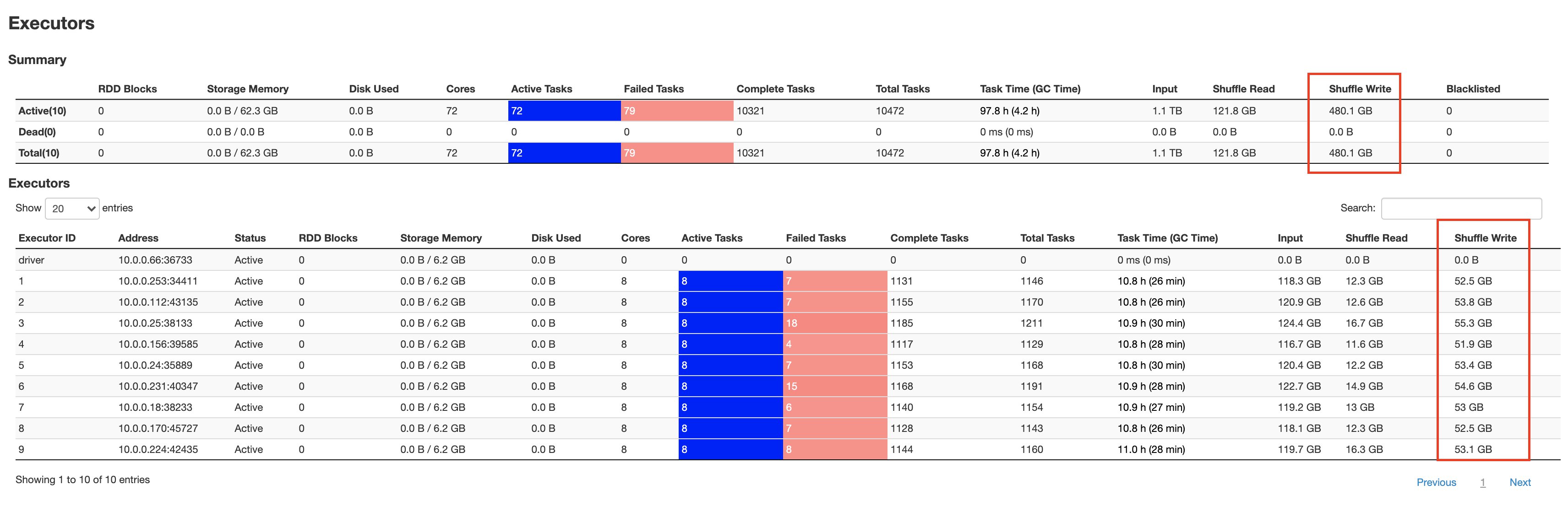
Rajendra Gujja is a Software Development Engineer on the AWS Glue team. He is passionate about distributed computing and everything and anything to do with the data.

Mohit Saxena is a Software Engineering Manager on the AWS Glue team. His team works on distributed systems for efficiently managing data lakes on AWS and optimizes Apache Spark for performance and reliability.