Organizations are increasingly expanding their Kubernetes footprint by deploying microservices to incrementally innovate and deliver business value faster. This growth places increased reliance on the network, giving platform teams exponentially complex challenges in monitoring network performance and traffic patterns in EKS. As a result, organizations struggle to maintain operational efficiency as their container environments scale, often delaying application delivery and increasing operational costs.
Today, I’m excited to announce Container Network Observability in Amazon Elastic Kubernetes Service (Amazon EKS), a comprehensive set of network observability features in Amazon EKS that you can use to better measure your network performance in your system and dynamically visualize the landscape and behavior of network traffic in EKS.
Here’s a quick look at Container Network Observability in Amazon EKS:
Container Network Observability in EKS addresses observability challenges by providing enhanced visibility of workload traffic. It offers performance insights into network flows within the cluster and those with cluster-external destinations. This makes your EKS cluster network environment more observable while providing built-in capabilities for more precise troubleshooting and investigative efforts.
Getting started with Container Network Observability in EKS
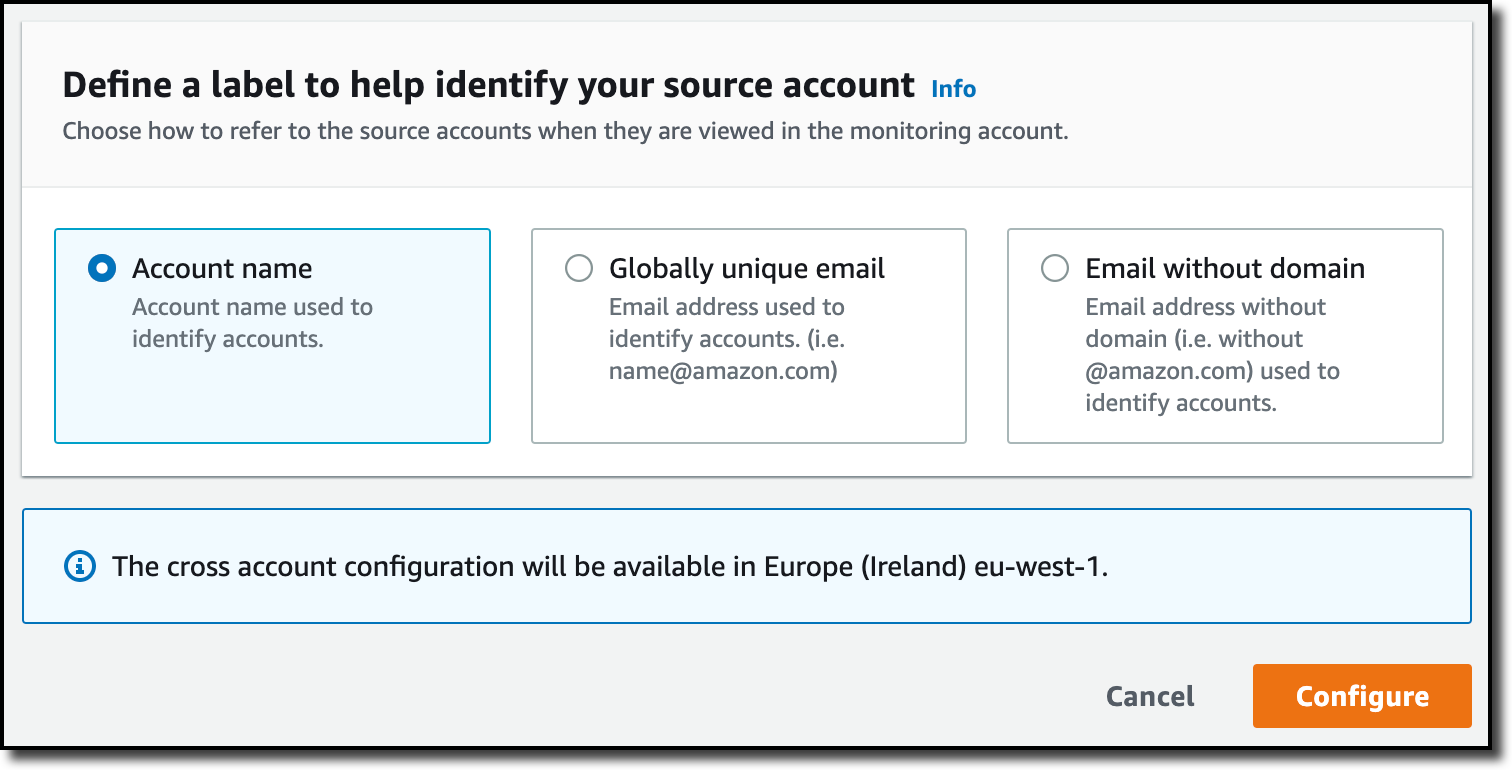
I can enable this new feature for a new or existing EKS cluster. For a new EKS cluster, during the Configure observability setup, I navigate to the Configure network observability section. Here, I select Edit container network observability. I can see there are three included features: Service map, Flow table, and Performance metric endpoint, which are enabled by Amazon CloudWatch Network Flow Monitor.
On the next page, I need to install the AWS Network Flow Monitor Agent.
After it’s enabled, I can navigate to my EKS cluster and select Monitor cluster.
This will bring me to my cluster observability dashboard. Then, I select the Network tab.
Comprehensive observability features Container Network Observability in EKS provides several key features, including performance metrics, service map, and flow table with three views: AWS service view, cluster view, and external view.
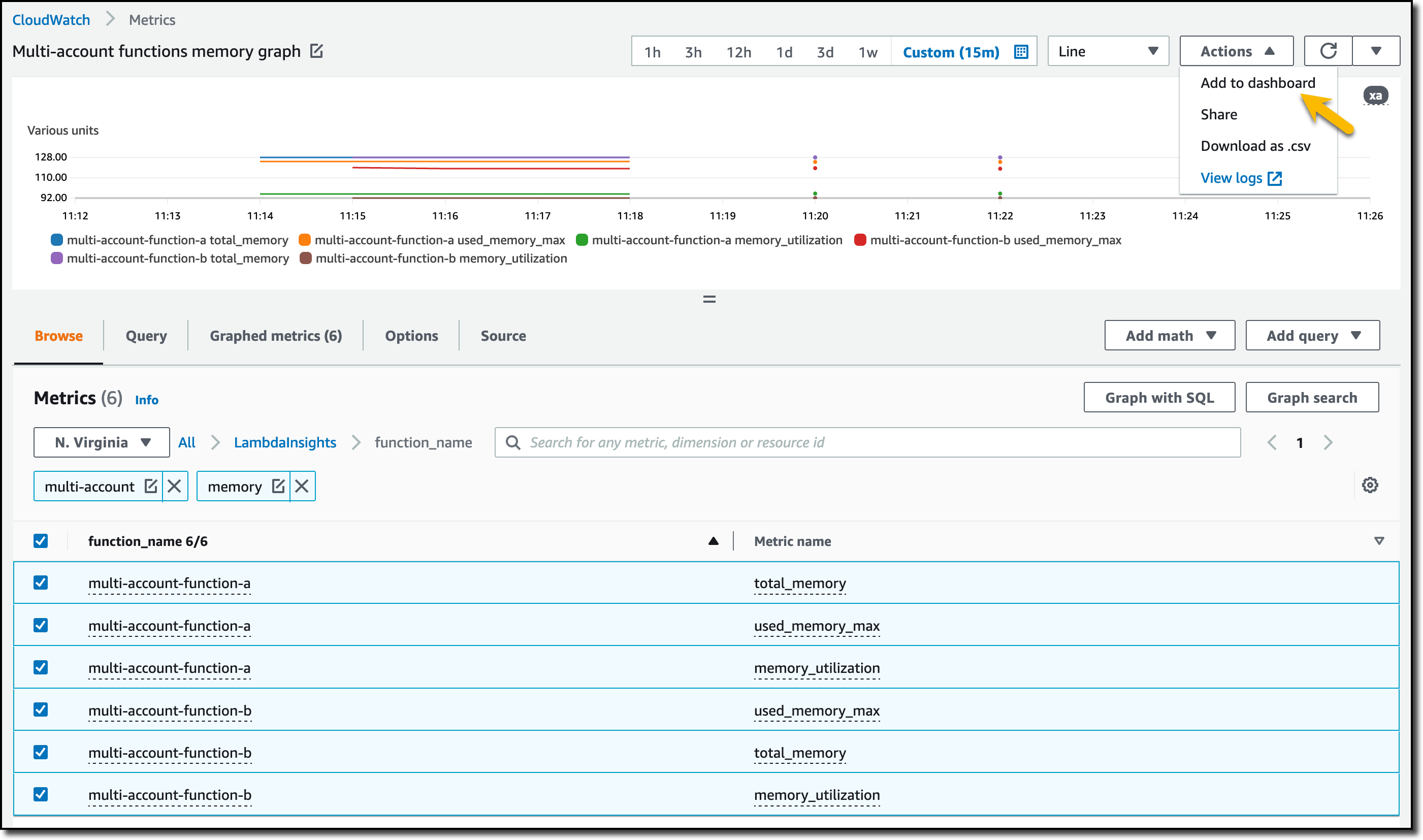
With Performance metrics, you can now scrape network-related system metrics for pods and worker nodes directly from the Network Flow Monitor agent and send them to your preferred monitoring destination. Available metrics include ingress/egress flow counts, packet counts, bytes transferred, and various allowance exceeded counters for bandwidth, packets per second, and connection tracking limits. The following screenshot shows an example of how you can use Amazon Managed Grafana to visualize the performance metrics scraped using Prometheus.
With the Service map feature, you can dynamically visualize intercommunication between workloads in your cluster, making it straightforward to understand your application topology with a quick look. The service map helps you quickly identify performance issues by highlighting key metrics such as retransmissions, retransmission timeouts, and data transferred for network flows between communicating pods.
Let me show you how this works with a sample e-commerce application. The service map provides both high-level and detailed views of your microservices architecture. In this e-commerce example, we can see three core microservices working together: the GraphQL service acts as an API gateway, orchestrating requests between the frontend and backend services.
When a customer browses products or places an order, the GraphQL service coordinates communication with both the products service (for catalog data, pricing, and inventory) and the orders service (for order processing and management). This architecture allows each service to scale independently while maintaining clear separation of concerns.
For deeper troubleshooting, you can expand the view to see individual pod instances and their communication patterns. The detailed view reveals the complexity of microservices communication. Here, you can see multiple pod instances for each service and the network of connections between them.
This granular visibility is crucial for identifying issues like uneven load distribution, pod-to-pod communication bottlenecks, or when specific pod instances are experiencing higher latency. For example, if one GraphQL pod is making disproportionately more calls to a particular products pod, you can quickly spot this pattern and investigate potential causes.
Use the Flow table to monitor the top talkers across Kubernetes workloads in your cluster from three different perspectives, each providing unique insights into your network traffic patterns.
Flow table – Monitor the top talkers across Kubernetes workloads in your cluster from three different perspectives, each providing unique insights into your network traffic patterns:
AWS service view shows which workloads generate the most traffic to Amazon Web Services (AWS) services such as Amazon DynamoDB and Amazon Simple Storage Service (Amazon S3), so you can optimize data access patterns and identify potential cost optimization opportunities.
The Cluster view reveals the heaviest communicators within your cluster (east-west traffic), which means you can spot chatty microservices that might benefit from optimization or colocation strategies
External viewidentifies workloads with the highest traffic to destinations outside AWS (internet or on premises), which is useful for security monitoring and bandwidth management.
The flow table provides detailed metrics and filtering capabilities to analyze network traffic patterns. In this example, we can see the flow table displaying cluster view traffic between our e-commerce services. The table shows that the orders pod is communicating with multiple products pods, transferring amounts of data. This pattern suggests the orders service is making frequent product lookups during order processing.
The filtering capabilities are useful for troubleshooting, for example, to focus on traffic from a specific orders pod. This granular filtering helps you quickly isolate communication patterns when investigating performance issues. For instance, if customers are experiencing slow checkout times, you can filter to see if the orders service is making too many calls to the products service, or if there are network bottlenecks between specific pod instances.
Additional things to know Here are key points to note about Container Network Observability in EKS:
Pricing – For network monitoring, you pay standard Amazon CloudWatch Network Flow Monitor pricing.
Availability – Container Network Observability in EKS is available in all commercial AWS regions where Amazon CloudWatch Network Flow Monitor is available.
Export metrics to your preferred monitoring solution – Metrics are available in OpenMetrics format, compatible with Prometheus and Grafana. For configuration details, refer to Network Flow Monitor documentation.
Amazon OpenSearch Serverless simplifies the deployment and management of OpenSearch workloads by automatically scaling based on your usage patterns. The service considers key metrics such as shard utilization, storage consumption, and CPU usage while maintaining millisecond-level response times, with the simplicity of a serverless environment.
While OpenSearch Serverless handles scaling automatically, implementing robust monitoring remains crucial for understanding usage patterns, optimizing costs, helping to ensure performance, and maintaining reliability. Proactive monitoring helps organizations detect critical issues with the applications or infrastructure in real time and identify root causes quickly.
This post is part of our Amazon OpenSearch service monitoring series, focusing on OpenSearch Serverless workloads and deployments. In this post, we explore commonly used Amazon CloudWatch metrics and alarms for OpenSearch Serverless, walking through the process of selecting relevant metrics, setting appropriate thresholds, and configuring alerts. This guide will provide you with a comprehensive monitoring strategy that complements the serverless nature of your OpenSearch deployment while maintaining full operational visibility.
Key benefits of CloudWatch monitoring for OpenSearch Serverless
Implementing CloudWatch monitoring for your OpenSearch Serverless collections offers several key advantages:
Near real-time performance monitoring – CloudWatch provides near real-time monitoring, enabling you to track your OpenSearch Serverless collections’ performance as they operate. This immediate visibility allows for swift detection of anomalies or performance issues, enabling prompt response to potential problems.
Efficient error diagnosis – You can quickly identify and address common errors without extensive log analysis. For instance, by monitoring ingestion request errors, you can preemptively mitigate bulk indexing request failures.
Proactive alerting system – Use the CloudWatch alarm functionality in conjunction with Amazon Simple Notification Service (SNS) to set up custom alerts. By defining specific thresholds for critical metrics, you can receive instant notifications through email or SMS when your OpenSearch Serverless collections approach or exceed these limits.
Comprehensive historical analysis – The data retention capabilities of CloudWatch allow for in-depth historical analysis. This helps you to identify long-term performance trends, recognize recurring patterns in resource utilization and optimize workload distribution based on historical insights.
Solution overview
Understanding which metrics to monitor in OpenSearch Serverless helps optimize your system’s performance and reliability. This guide explains the key metrics to monitor, their significance, how to determine appropriate thresholds, and the step-by-step process for setting up alarms. Understanding these fundamentals will help you establish effective monitoring for your OpenSearch Serverless collections and help maintain optimal performance and reliability.
Prerequisites
Before getting started, you must have the following prerequisites:
An AWS account that provides access to AWS services.
CloudWatch metrics and recommended alarms for OpenSearch Serverless
The following table summarizes key CloudWatch metrics for OpenSearch Serverless, including recommended alarm thresholds, metric descriptions, and applicable workload types.
Alarm
Metric Level
Metric Description
Alarm Description
Use case
IndexingOCU maximum is >= 10 for 5 minutes, three consecutive times
Account Level
Serverless compute capacity is measured in OpenSearch Compute Units (OCUs). Each OCU is a combination of 6 GiB of memory and corresponding virtual CPU (vCPU), in addition to data transfer to Amazon Simple Storage Service (Amazon S3).
The IndexingOCU metric reports the number of OCUs used for data ingestion across all collections.
This alarm will alert you when Indexing OCUs scale upto / beyond 10 for more than 15 minutes.
Monitor and Optimize Costs
SearchOCU maximum is >= 10 for 5 minutes, three consecutive times
Account Level
Serverless compute capacity is measured in OCUs. Each OCU is a combination of 6 GiB of memory and corresponding virtual CPU (vCPU), in addition to data transfer to Amazon S3.
The SearchOCU metric reports the number of OCUs used to search collection data across all collections.
This alarm will alert you when Search OCUs scale upto / beyond 10 for more than 15 minutes.
Monitor and Optimize Costs
IngestionRequestLatency maximum is >= 3 secs for 1 minutes, five consecutive times.
Collection Level
The IngestionRequestLatency metric reports the latency, in seconds, for bulk write operations to a collection.
This alarm monitors the maximum latency of bulk write operations to a collection. It triggers when the maximum IngestionRequestLatency exceeds 3 seconds for five consecutive 1-minute intervals (for a total of 5 minutes). This indicates a sustained performance degradation in data ingestion operations, which could impact application performance and data availability.
This metric might be crucial to monitor for log-based workloads, where indexing time is critical.
SearchRequestLatency maximum is >= 2 secs for 1 minutes, five consecutive times.
Collection Level
The SearchRequestLatency metric reports the latency, in seconds, that it takes to complete a search operation against a collection.
This alarm monitors the maximum latency of search operations against a collection. It triggers when the maximum SearchRequestLatency exceeds 2 seconds for five consecutive 1-minute intervals (for a total of 5 minutes). Consistently high search latency indicates performance issues that could degrade user experience and application responsiveness.
This metric might be crucial to monitor for vector and search-based workloads, where search time is critical.
IngestionRequestErrors sum is >= 100 errors for 1 minute, five consecutive times
Collection Level
The IngestionRequestErrors metric reports the total number of bulk indexing request errors to a collection. OpenSearch Serverless emits this metric when there are bulk indexing request failures, such as an authentication or availability issue.
This alarm monitors the total count of failed bulk indexing operations to a collection. It triggers when the number of IngestionRequestErrors equals or exceeds 100 errors for five consecutive 1-minute intervals (for a total of 5 minutes).
Persistent ingestion errors indicate systemic issues that could lead to data loss or inconsistency.
SearchRequestErrors sum is >= 50 errors for 1 minute, five consecutive times
Collection Level
The SearchRequestErrors metric reports the total number of query errors per minute for a collection.
This alarm monitors the total count of failed search query operations in a collection. It triggers when the number of SearchRequestErrors equals or exceeds 50 errors for five consecutive 1-minute intervals (for a total of 5 minutes).
Persistent search errors indicate potential issues that could impact application functionality and user experience.
ActiveCollection minimum is 0 for 1 minutes, three consecutive times.
Collection Level
This metric indicates whether a collection is active. A value of 1 means that the collection is in an ACTIVE state. This value is emitted upon successful creation of a collection and remains 1 until you delete the collection. The metric can’t have a value of 0.
The alarm triggers when the metric is missing for three consecutive 1-minute intervals (for a total of 3 minutes). Because an active collection always emits a value of 1, missing data indicates the collection has been deleted or is experiencing serious issues. Note: Make sure to setup the CloudWatch alarm so that it will treat missing data as breaching.
Monitor Availability of Collection
The specific threshold values mentioned are examples. However, you may need to adjust these thresholds based on the unique requirements and SLAs of your own applications and workloads running on OpenSearch Serverless.
To decide when to raise the global OCU limits, you should regularly review the IndexingOCU and SearchOCU metrics at the account level. If you notice the metrics consistently approaching the set threshold, it’s a good indication that you should consider increasing the overall account limits to accommodate your growing usage.
Additionally, monitor the collection-level metrics like IngestionRequestLatency and SearchRequestLatency. If you notice certain collections have consistently high latency, it might be a sign that the OCU allocation for those specific collections is insufficient. In such cases, you could consider increasing the OCU limits for those high-usage collections, rather than raising the global account limits.
By closely monitoring both the account-level and collection-level metrics, you can make informed decisions about when and how to adjust your OCU limits to maintain optimal performance and cost efficiency for your OpenSearch Serverless deployment.
Steps to create a CloudWatch alarm
CloudWatch Alarms can be created using any of the following methods:
Detailed steps and a / sample code snippet for each method are provided in the following sections.
Using the console
The AWS Management Console provides a user-friendly, visual interface for creating CloudWatch alarms. Follow these step-by-step instructions to set up your alarm through the console.
In the navigation pane, choose Alarms and then, All alarms.
Choose Create alarm.
Choose Select Metric.
Select the namespace AOSS
To setup alerting on IndexingOCU across all collections, navigate to ClientId and select the metric.
Under Conditions:
For Statistic: Select Maximum.
For Period: Select 5 minutes.
For Threshold type: Choose Static and Greater.
Choose Next. Under Notification, select an SNS topic to notify when the alarm is in ALARM state, OK state, or INSUFFICIENT_DATA state.
When finished, choose Next. Enter a name and description for the alarm. The name must contain only UTF-8 characters, and can’t contain ASCII control characters. The description can include markdown formatting, which is displayed only in the alarm Details tab in the CloudWatch console. The markdown can be useful to add links to runbooks or other internal resources. Then choose Next.
Under Preview and create, confirm that the information and conditions are what you want, then choose Create alarm.
For those who prefer command-line interfaces or need to automate alarm creation, the AWS CLI offers an efficient alternative. This section demonstrates how to create a CloudWatch alarm using a single CLI command.
To set up a CloudWatch alarm using the AWS CLI, you can use the put-metric-alarm command. The following example demonstrates how to create an alarm that sends an Amazon SNS email when the IndexingOCU exceeds 2 for 15 minutes at the account level. Replace [region] and [account-id] with your AWS Region and account ID.
Infrastructure as Code (IaC) enables version-controlled, repeatable deployments. This JSON template shows how to define a CloudWatch alarm using AWS CloudFormation, suitable for those who prefer JSON syntax for their IaC implementations.
Replace [region] and [account-id] with your AWS Region and account ID.
For teams that prefer YAML’s more readable format, this section provides the equivalent CloudFormation template in YAML. The template creates the same CloudWatch alarm with identical configurations as the JSON version.
Replace [region] and [account-id] with your AWS Region and account ID.
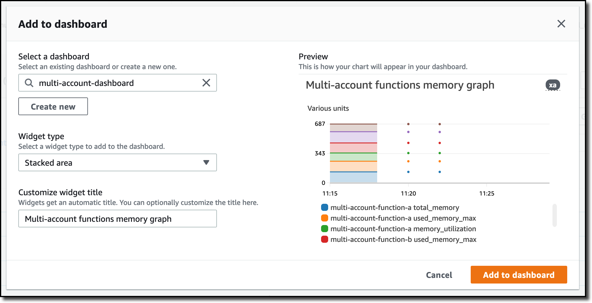
You can use Amazon CloudWatch dashboards to monitor multiple resources in a unified view. For example, the following dashboard provides a consolidated view of OpenSearch Serverless OCU usage, helping you track and manage costs.
Clean up
To avoid incurring unintended future charges, delete the following resources that were created as part of solution walk-through of this post:
CloudWatch alarms
CloudFormation stacks
SNS topics
Conclusion
Effective monitoring helps maintain optimal performance and reliability of your OpenSearch Serverless collections. By implementing the CloudWatch alarms and monitoring strategies outlined in this post, you can work towards proactively identifying and responding to performance issues before they impact your applications, optimize costs by tracking OCU usage patterns, support high availability objectives by monitoring collection health and error rates, and help maintain consistent performance through latency monitoring. Remember that the thresholds suggested in this guide serve as a starting point, you should adjust them based on your specific use cases, performance requirements, and budget constraints. Regular review and refinement of these alarms will help you maintain an efficient and cost-effective OpenSearch Serverless deployment.
Zapier is a leading no-code automation provider whose customers use their solution to automate workflows and move data across over 8,000 applications such as Slack, Salesforce, Asana, and Dropbox. Zapier runs these automations through integrations called Zaps, which are implemented using a serverless architecture running on Amazon Web Services (AWS). Each Zap is powered by an AWS Lambda function.
In this post, you’ll learn how Zapier has built their serverless architecture focusing on three key aspects: using Lambda functions to build isolated Zaps, operating over a hundred thousand Lambda functions through Zapier’s control plane infrastructure, and enhancing security posture while reducing maintenance efforts by introducing automated function upgrades and cleanup workflows into their platform architecture.
Architecting a secure and isolated runtime environment
Zaps created by Zapier’s users implement tenant-specific business logic, hence they require cross-tenant compute isolation. Code implementing one Zap can’t share an execution environment with code implementing another Zap. Moreover, the same Zap type used by two different tenants can’t share execution environments as well.
To achieve the required level of isolation, Zapier’s engineering team adopted AWS Lambda, a serverless compute service that runs code in response to events and automatically manages cloud compute resources. Minimal operational overhead, built-in high availability, automated scaling, high level of isolation, and pay-per-use model made Lambda a great fit for this use case. Currently, Zapier’s architecture is running over a hundred thousand Lambda functions to support their customer’s integration workflows.
Because they’re powered by the open source Firecracker microVMs, each function is completely isolated from the others. Moreover, each execution environment belonging to the same function (sometimes referred to as function instances) is also isolated from other execution environments. The following architecture topology diagram uses red lines to represent isolation boundaries. Each execution environment of every function is isolated from its peers and is getting its own virtual resources such as disk, memory, and CPU. For more details, read Security in AWS Lambda.
Zapier’s control plane is architected using Amazon Elastic Kubernetes Service (Amazon EKS). A designated database is used to maintain the up-to-date function inventory. Whenever a user creates a new Zap, the control plane creates a corresponding Lambda function and stores a reference in the inventory database. When a Zap is triggered, the control plane retrieves information about a relevant Lambda function and invokes it to facilitate the integration workflow, as illustrated in the following diagram.
Understanding the runtime deprecation process
When building architectures using the traditional non-serverless compute, cloud engineers are the ones responsible for keeping operating systems and software on their compute instances up to date and applying security and maintenance patches. With serverless architectures and Lambda functions, security patches and minor runtime upgrades are handled by AWS automatically, which means customers can focus on delivering business value instead of the undifferentiated heavy lifting of infrastructure management.
As Zapier’s user base and architectural complexity – and consequently the number of Zaps – were growing, keeping all functions on the most up-to-date major runtime versions became a laborious task. Top contributing factors were:
High number of functions. At its peak, the Zapier platform was running Zaps using hundreds of thousands of unique Lambda functions. Approximately 35% of these functions were using a runtime that was scheduled for deprecation in the next 12 months.
Zapier architected their data plane environment to be ephemeral – the control plane creates and deletes Lambda functions on demand and manages their lifecycle dynamically. Identifying a specific owner for each affected function wasn’t always straightforward.
Security is paramount at Zapier and upgrading affected functions runtime prior to the deprecation date was an absolute must. At no point could Zapier functions use runtimes after their deprecation date. This was a task which required extra resources.
The upgrade process shouldn’t have had any impact on the end customer experience. At no point should customer experience be affected.
With a short runway, high-volume workload, and the strict requirements of not impacting customer experience, Zapier’s Platform Engineering team took on this challenge of maintaining high security posture in their platform architecture.
Applying the solution
The solution had three work streams:
Reducing the risk by analyzing the architecture and identifying and cleaning up unused functions.
Prioritizing upgrades by identifying the most critical and impactful functions.
Empowering engineering teams with automated tools and knowledge to streamline the upgrade process in future.
Identify and clean up unused functions
The first step in streamlining the upgrade process was identifying and removing unused functions. This reduced the total number of functions in Zapier’s architecture that required upgrades, eliminating unnecessary work for the team.
This meant the team could build a detailed inventory of functions that were running on soon-to-be deprecated runtimes. Using Amazon CloudWatch, Zapier’s platform team started to monitor metrics such as number of invocations. They identified which functions were active, which functions weren’t used for an extended period, and which functions didn’t have an active owner and could be removed.
One of the primary mechanisms for ownership validation within the organization was using resource tags. Functions that were active, but didn’t have clear ownership, were flagged for additional review before removal. Functions that were confirmed as unused or didn’t have an active owner were marked for deletion. Removing such functions allowed Zapier to significantly simplify their architecture and reduce the number of functions that had to be upgraded.
Prioritizing upgrades
With a smaller volume of functions to upgrade, Zapier’s platform team prioritized function upgrades based on usage patterns, criticality, and potential customer impact. Three primary prioritization categories were:
Customer-facing functions – Any functions directly involved in executing user Zaps were marked as high priority. These had to be upgraded first to avoid service disruptions.
Backend infrastructure functions – Internal functions that supported system operations were evaluated based on their importance to platform stability.
High-volume functions – Functions with the highest execution frequency were prioritized because upgrading them would have the greatest impact on reducing operational risk.
Using these factors, Zapier’s platform team has created an upgrade roadmap, ensuring that critical assets were addressed first while minimizing potential disruptions.
Empowering engineering teams with automated tools and knowledge
To ensure a smooth and efficient upgrade process across their serverless architecture, Zapier’s team empowered engineering teams with clear guidelines and automated solutions. The platform incorporated two main approaches: Terraform-managed functions and a custom-built Lambda runtime canary tool. Implementing and adopting these tools and practices resulted in reducing the number of functions using soon-to-be deprecated runtimes by 95%.
For functions managed through infrastructure-as-code (IaC), Zapier’s team developed standardized Terraform modules that specified supported runtime versions. Development teams implemented these modules in their configurations:
After applying the new module version, teams validated changes by testing the new runtime in staging environments and monitoring Terraform plan outputs to ensure proper runtime version updates.
To efficiently manage most Lambda functions in their architecture, Zapier developed the Lambda runtime canary tool suite. Using this solution, they automated the runtime upgrade process for thousands of active Lambda functions with minimal manual intervention. The tool suite implements several key features:
Architected for gradual traffic shifting with the Lambda built-in routing mechanism through function version and aliasing. The tool can gradually shift traffic distribution from an old to a new function version. During this gradual traffic shift, the system monitors CloudWatch metrics for errors and automatically rolls back if error rates exceed acceptable thresholds.
Optimistic upgrade strategy implements direct upgrades for infrequently used functions using a flag value stored in a cache to detect potential issues during the first post-upgrade invocation. If this invocation fails, the control plane retries it using the previous function version. If the retried invocation succeeds, Zapier’s control plane initiates a rollback, assuming the error is most likely due to the runtime upgrade. After rollback, it will log the error and alert relevant stakeholders.
Integration with existing infrastructure uses an administrative interface and task queue for automated traffic shifting. A database ledger maintains tracking of function states and rollback information.
Operational controls provide manual rollback capabilities and implement centralized control switches for process management. After a function was upgraded to a new runtime and no rollback activity was detected within a set time period, an automated pruning task cleans up older versions.
Zapier’s Lambda canary tool, through its integration of gradual traffic shifting, real-time CloudWatch monitoring, and automated rollback mechanisms, established a sustainable framework for managing runtime upgrades across their serverless architecture. This approach not only automated the upgrade process and minimized operational risks but also created a scalable solution that provides continuous runtime upgrades, preventing the use of deprecated runtimes at any point. By allowing continuous function runtime updates with minimal disruption to end user experience, Zapier maintains security and stability while requiring minimal manual intervention. This framework efficiently manages their growing serverless infrastructure, providing both security and operational efficiency for future runtime updates.
Conclusion
In this post, you’ve learned how Zapier architected their software-as-a-service (SaaS) platform to provide secure, isolated execution environments using AWS Lambda and Amazon EKS, enabling their customers to create hundreds of thousands of Zaps. You’ve learned how Zapier’s team implemented the function runtime upgrade process at scale and reduced the number of functions running on soon-to-be deprecated runtimes by 95%. You’ve seen best practices that were established and techniques that helped Zapier to keep high security posture without impacting customer experience.
Use the following links to learn more about Lambda runtimes and upgrading your functions to the latest runtime versions:
Infrastructure alerts pose a challenge for DevOps teams, particularly when they occur outside of regular business hours. The complexity isn’t merely in receiving notifications, it lies in rapidly assessing their severity and determining the root cause. This challenge is compounded when upstream service disruptions cascade into multiple downstream alerts, creating a confusion of notifications that mask the true source of the problem. DevOps teams find themselves working backwards through a complex web of interconnected services, unsure whether to start investigating at the application, network, or infrastructure level.
To reduce resolution time and alert root cause analysis, AWS introduced CloudWatch Investigations, a generative AI-powered capability within Amazon CloudWatch. Powered by Amazon Q Developer, a generative AI–powered assistant for software development, CloudWatch investigations analyzes multiple metrics, logs, and deployment events to provide suggestions for remediation and root-cause analyses, reducing alarm resolution time. A key advantage of this feature is the ability to integrate these findings directly into Microsoft Teams and Slack, making sure developers and stakeholders receive immediate alerts when issues arise. This centralized collaboration approach enables teams to work together efficiently, reducing duplicate efforts and facilitating consistent problem-solving across the organization.
In this blog post, we will walk through how to integrate CloudWatch Investigations with Slack channels and demonstrate how to interact with investigations in Slack.
Overview of the solution
CloudWatch Investigations can be started in multiple ways, like from existing Amazon CloudWatch log insights, metrics, or alarms. To demonstrate CloudWatch Investigations functionalities, we will use CloudWatch alarms in a sample web application available in the aws-samples GitHub repository. Steps on how to deploy this web app in your AWS environment, via a CloudFormation template, can be found here. You can learn more about the architecture of the resources deployed in the AWS One Observability workshop. If you choose to deploy the sample web application, you will be responsible for all service charges associated with the CloudFormation template deployment. Alternatively, you can use existing CloudWatch alarms in your environment. Examples of common Amazon CloudWatch alarms include: MemoryUtilization, CPUUtiliziation, 5xxErrors and 4xxError. A full list of available alarms can be found here.
For this blog, we will utilize a pre-configured alarm to monitor when one of the website services, backed by an Application Load Balancer, experiences abnormal response times. When the alarm triggers, CloudWatch Investigations automatically initiates an investigation, analyzing both the current alarm state and 90 days of CloudTrail event history to generate hypotheses and determine potential root causes. The investigation insights are published to a Slack channel via Amazon Q Developer in Chat Applications and Amazon Simple Notification Service (SNS).
Figure 1. Architecture diagram of the services involved in the investigation integration in Slack
Prerequisites
Launch the Amazon CloudFormation template associated with the One Observability lab outlined in the AWS Samples GitHub.
Set up a Standard Amazon SNS topic by following the instructions outlined here. To enable CloudWatch investigations to send notifications to Slack, you must add an access policy to the Amazon SNS topic, an example can be found here.
When the topic configuration is complete, navigate to Amazon Q Developer in Chat Applications (formerly AWS Chatbot) to configure the integration between Amazon Q and Slack by following the instructions outlined here. To allow channel members to interact with the investigation in Slack, add the following permission templates to the Channel role settings: Notification Permissions, Amazon Q Permissions, and Amazon Q Operations assistant permissions. More details on these permissions can be located here.
Setting up CloudWatch Investigations
To get started, navigate to the Amazon CloudWatch console. Choose AI Operations and then Configuration.
Figure 2. Configure for this account button within the AWS Console
Before we can set up an investigation, we need to create an investigation group. This is an organizational structure to manage common properties of the investigation like retention requirements, encryption, access permissions and the SNS topic linked. Click Configure for this account and follow the prompts in the console to set up the investigation group. Detailed explanations for each prompt are located in the documentation here. For this demo, we left the default options for steps 1 and 2 of the prompts. In step 3, please select the existing SNS topic created in the prerequisites section.
Figure 3. Select SNS topic for Q Developer Operational Insights
For the investigation trigger, we will use an existing alarm created by the CloudFormation deployment mentioned at the beginning of this blog. The sample alarm is named:
and it goes into ALARM state when one of the website services, backed by an Application Load Balancer, experiences abnormal response times.
To configure this alarm to automatically start an investigation when it goes into an ALARM state:
In the CloudWatch console, choose Alarms, All alarms
Search for the alarm name and click on it
Choose Actions, Edit
Choose Next once to skip the metrics and conditions section
Choose Add investigation action and then select your investigation group as outlined in figure 4
Choose Skip to Preview and create, then choose Update alarm
Figure 4. Configure alarm to automatically start investigations
Testing the solution
At this point, we are ready to test the solution. To simulate a website traffic overload and trigger the alarm, we are going to use Amazon ECS tasks deployed as part of the sample web application. Open up CloudShell and run the following command:
The command will launch 5 instances of the Amazon ECS traffic generator container task. Once the tasks are running (after about 5 minutes), the ALB will become overloaded with requests, forcing the alarm into ALARM state as shown below. You should also see a new investigation created.
Figure 5. CloudWatch Alarm in ALARM state
Interacting with the investigation via Slack
Once the alarm is triggered, an investigation is initiated. Since we associated the investigation with an Amazon SNS topic and subscribed our Slack client to it, we can see a message in our Slack channel from Amazon Q as seen in figure 6.
Figure 6. Slack notification for open investigation
Within Slack, channel members can accept useful hypotheses and discard unhelpful ones by clicking on the Accept or Discard button. They can also add text-based notes of observations or evidence to the investigation by clicking on the Add Note button. Amazon Q will respond to messages within the same thread as the original investigation message. Channel members will be able to track who has accepted or discarded messages, as well as notes made about the investigation. This emphasizes the power of Slack integration, as teams can collaborate on the investigation and track who is actively working on it. It is important to note that CloudWatch Investigations uses Generative AI and may provide suggestions different from those below based on your specific account environment.
Figure 7. Accept or discard investigation suggestions from Slack
When integrated with Slack, CloudWatch Investigations can provide suggestions and root-cause hypotheses. Channel members with appropriate permissions can access metrics, charts, and additional information related to the investigation by clicking the blue header at the top of the investigation message. This link will direct users to the CloudWatch Investigations feed in the AWS console as shown below in figure 8.
Figure 8. CloudWatch Investigations in CloudWatch console.
Integrating CloudWatch Investigations with Slack or Teams channels improves developers’ visibility of arising issues and provides targeted recommendations to reduce alarm resolution time. The Accept and Discard buttons make it straightforward to track who is actively working on an investigation, fostering a culture of collaboration. The best part? The integration is quick to set up, especially with existing alarms.
Clean Up
If you launched the CloudFormation template mentioned at the beginning of this blog, the services will continue to run unless you delete them. To make sure that you are not charged for use of the resources after the demo, please follow the below steps to delete the resources created as part of the steps performed on this blog.
Remove the Amazon Q in Chat Applications Slack integration by clicking on Remove Workspace Integration and policy as explained here.
Delete Amazon SNS topic and subscription as explained here.
Remove the CloudWatch Investigations as explained here.
Delete the images under the Amazon ECR repository named cdk-…-container-assets… as explained here.
Open the CloudShell console or AWS CLI and execute the two commands below:
After executing the above command, the resources of the demo should be destroyed. Look at the CloudFormation console in case of potential errors.
Conclusion
The new CloudWatch Investigations feature reduces alarm resolution time for development teams by providing actionable insights and recommendations. It is straightforward to connect investigations to a team’s primary form of communication, such as Teams or Slack, to improve notification awareness and interaction. To learn more about the capabilities of CloudWatch Investigations check out the feature announcement and documentation.
Running applications across hybrid or multicloud environments creates a common challenge: fragmented logs scattered across different platforms. This fragmentation complicates monitoring, slows troubleshooting, and reduces operational visibility. To address this, many organizations seek to implement secure log ingestion from all environments into a centralized platform.
Amazon OpenSearch Service provides a unified solution for real-time search, analytics, and log management across your entire infrastructure. Amazon OpenSearch Ingestion, a fully managed data collector, simplifies data processing with built-in capabilities to filter, transform, and enrich your logs before analysis.
However, securely sending logs from non-AWS environments presents a challenge. Every request to OpenSearch Ingestion requires AWS Signature Version 4 (AWS SigV4) authentication, traditionally requiring long-term credentials that introduce security risks. AWS Identity and Access Management Roles Anywhere solves this problem by providing temporary credentials for workloads running outside AWS.
In this post, we demonstrate how to configure Fluent Bit, a fast and flexible log processor and router supported by various operating systems, to securely send logs from any environment to OpenSearch Ingestion using IAM Roles Anywhere. This approach alleviates the need for long-term credentials while providing a comprehensive view of your application logs across all environments—improving security, simplifying operations, and enhancing your ability to quickly resolve issues.
Solutions overview
The solution in this post uses Fluent Bit to collect logs, retrieve temporary credentials from IAM Roles Anywhere, and sign HTTP log ingestion requests with AWS SigV4 before sending them to the OpenSearch Ingestion pipeline. The following diagram shows the architecture.
This solution provisions the following key components:
IAM Roles Anywhere configuration – This includes the following:
Trust anchor – Establishes trust between IAM Roles Anywhere and the specified CA.
IAM role – Grants permissions for log ingestion and trusts the IAM Roles Anywhere service principal. At minimum, this role must be granted permission for the osis:Ingest action.
Profile – Defines which roles IAM Roles Anywhere can assume and the maximum permissions granted with the temporary credentials.
OpenSearch Service domain – For this post, we use an OpenSearch Service domain, which is an AWS provisioned equivalent of an open source OpenSearch cluster. We create the domain within a virtual private cloud (VPC); see VPC versus public domains for more information. Alternatively, you can use an Amazon OpenSearch Serverless collection, which is an OpenSearch cluster that scales compute capacity based on your application’s needs.
OpenSearch Ingestion – This is configured to receive logs over HTTP as the pipeline source and forward them to the OpenSearch Service domain as the pipeline sink.
Connectivity between AWS and your hybrid or multicloud environments
You can access your OpenSearch Ingestion pipelines using an interface VPC endpoint with push-based HTTP source, which provides private IP address connectivity. For production environments, we recommend using these private connections through interface endpoints for enhanced security.
Setting up this connectivity requires additional configuration, such as creating an AWS Site-to-Site VPN connection with your hybrid and multicloud network. Although this post focuses on the log ingestion solution, you can find detailed guidance on network connectivity in the following resources:
Hybrid connectivity – Learn about different methods to connect your on-premises networks to AWS
How Fluent Bit retrieves temporary credentials using IAM Roles Anywhere
Using the HTTP output plugin, Fluent Bit can send logs to the OpenSearch Ingestion pipeline. The following diagram is a simplified view of how Fluent Bit retrieves AWS credentials.
On Linux systems, Fluent Bit can use an AWS Command Line Interface (AWS CLI) profile that uses the credential_process parameter to trigger an external process. This external process is invoked to generate or retrieve credentials not directly supported by the AWS CLI.
The following are two common mechanisms for the external process:
As of this writing, the Fluent Bit aws_profile configuration is supported only on Linux. It is untested on other Unix-based systems (such as macOS) and is not implemented for Windows.
Prerequisites
Before you begin this walkthrough, make sure you have the following:
Access to AWS CloudShell for exporting a sample private certificate we will create using AWS CloudFormation in a later step.
Remote (hybrid or multicloud) environment – You must have a remote machine with Linux-based operating system. This solution was tested on Ubuntu 24.04 with the following additional tooling installed:
Follow these steps to deploy AWS resources required for this solution:
Choose Launch Stack:
Enter a unique name for Stack name. The default value is osis-with-iamra.
Configure the stack parameters. Default values are provided in the following table.
Parameter
Default value
Description
CACommonName
example.com
Common Name for the CA
CACountry
US
Organization for the CA
CAOrganization
Example Org
Country for the CA
CAValidityInDays
1826
Validity period in days for the CA certificate
VPCCIDR
10.0.0.0/16
IPv4 CIDR range for the VPC used for OpenSearch Service domain
PublicSubnetCIDR
10.0.0.0/24
IPv4 CIDR range for public subnet
PrivateSubnet1CIDR
10.0.1.0/24
IPv4 CIDR range for private subnet
PrivateSubnet2CIDR
10.0.2.0/24
IPv4 CIDR range for private subnet
DomainName
test-domain
Name of the OpenSearch Service domain
PipelineName
test-pipeline
Name of the OpenSearch Ingestion pipeline
PipelineIngestionPath
/test-ingestion-path
Ingestion path for the OpenSearch Ingestion pipeline
Select the acknowledgement check box and choose Create Stack. Stack deployment takes about 30 minutes to complete.
When stack creation is complete, navigate to the Outputs tab on the AWS CloudFormation console and note down the values for the resources created. The following table summarizes the output values.
Output
Description
Example value
ACMCertificateArn
Amazon Resource Name (ARN) of the ACM certificate. You will use this for exporting certificate and private key files using the AWS CLI in a later step.
Export the certificate ARN from the CloudFormation outputs. If you changed the stack name in the previous step, use that value for <stack-name>, otherwise use the default value osis-with-iamra.
Create a new profile named osis-pipeline-credentials that invokes the credential process. Replace the placeholders with your specific values. Find the values for trusted-anchor-arn, profile-arn, and ingestion-role-arn in your CloudFormation stack outputs.
Run the following command to create a Fluent Bit configuration. Replace the placeholders with your specific values. Find the osis-pipeline-endpoint and pipeline-ingestion-path values in your CloudFormation stack outputs.
cat << 'EOF' > ~/fluent-bit.conf
[INPUT]
  name                  tail
  path                  /var/log/syslog
  read_from_head        true
  refresh_interval      5
[OUTPUT]
  name 			http
  match	   		*
  aws_service 		osis
  host 			<osis-pipeline-endpoint>
  port 			443
  uri 			<pipeline-ingestion-path>
  format 		json
  aws_auth	 	true
  aws_region 		<aa-example-1>
  aws_profile 		osis-pipeline-credentials
  tls 			On
EOF
This example configuration includes the following:
Uses the tail input plugin to monitor the /var/log/syslog file
Uses the http output plugin to flush log records to the OpenSearch Ingestion pipeline endpoint
Uses the osis-pipeline-credentials profile to obtain temporary AWS credentials for SigV4 authentication (aws_auth set to true)
Test the solution
Follow these steps to test the setup:
Start the Fluent Bit client with the configuration file fluent-bit.conf that you created in the previous step. Replace the placeholder with the value applicable to your environment. For Ubuntu 24.04, the default path of the Fluent Bit client is /opt/fluent-bit/bin/fluent-bit. Adjust the path if using other distributions.
Because the solution in this post launched the OpenSearch Service domain within a VPC, you will need an environment that has connectivity to the VPC. For this post, we create a CloudShell VPC environment to run the commands in the next step. Find the VPC, subnet, and security group to use from your CloudFormation stack outputs.
The solution that you deployed through AWS CloudFormation dynamically creates indexes based on ingestion timestamps, format logs-%{yyyy.MM.dd}. You can specify your preferred naming using OpenSearch Ingestion index management. You can query your OpenSearch index using your preferred tool to see the ingested logs from Fluent Bit. We use awscurl in a CloudShell environment as shown in the following example. Replace the placeholders with your specific values. Find the opensearch-domain-endpoint value in your CloudFormation stack outputs.
pip install awscurl

export OPENSEARCH_DOMAIN_ENDPOINT=https://<opensearch-domain-endpoint>

# List indices matching logs-%{yyyy.MM.dd} format and get most recent one to query
export INDEX=$(awscurl --service es "$OPENSEARCH_DOMAIN_ENDPOINT/_cat/indices?v" | grep -E "logs-[0-9]{4}\.[0-9]{2}\.[0-9]{2}" | sort -r | head -1 | awk '{print $3}')

awscurl --service es $OPENSEARCH_DOMAIN_ENDPOINT/$INDEX/_search \
        -X GET -H "Content-Type: application/json" \
        -d '{
            "size": 10,
            "sort": [
              {"@timestamp": {"order": "desc"}}
            ],
            "query": { "match_all": {} }
          }' | jq '.hits.hits[]._source'
The following is an example of the expected output:
In this post, we demonstrated how to obtain temporary credentials from IAM Roles Anywhere and securely ingest logs from hybrid or multicloud environments into OpenSearch Service using OpenSearch Ingestion. This approach minimizes the risk of credential exposure while enabling centralized log collection from distributed workloads. This solution is particularly valuable for organizations managing complex infrastructures across multiple environments and looking to consolidate observability data in OpenSearch Service. For additional details, refer to the following resources:
If you have questions or feedback about this post, please leave them in the comments section.
About the Authors
Xiaoxue Xu is a Solutions Architect for AWS based in Toronto. She primarily works with financial services customers to help secure their workload and design scalable solutions on the AWS Cloud.
Simran Singh is a Senior Solutions Architect at AWS. In this role, he assists our large enterprise customers in meeting their key business objectives using AWS. His areas of expertise include artificial intelligence and machine learning, security, and improving the experience of developers building on AWS.
Troubleshooting a large, complex, distributed enterprise application involves challenges like tracing requests across multiple services, identifying performance bottlenecks across the stack, and understanding cascading failures between dependent services. Customers often need to work with isolated data to identify the underlying cause of the problem. By correlating different signals like logs, traces, metrics, and other performance indicators, you can get valuable insight into what caused the problem, where, and why.
Amazon OpenSearch Service is a managed service to deploy, operate, and search data at scale within AWS. Amazon Managed Grafana is a secure data visualization service to query operational data from multiple sources, including OpenSearch Service.
In this post, we show you how to use these services to correlate the various observability signals that improve root cause analysis, thereby resulting in reduced Mean Time to Resolution (MTTR). We also provide a reference solution that can be used at scale for proactive monitoring of enterprise applications to avoid a problem before they occur.
Solution overview
The following diagram shows the solution architecture for collecting and correlating various enterprise telemetry signals at scale.
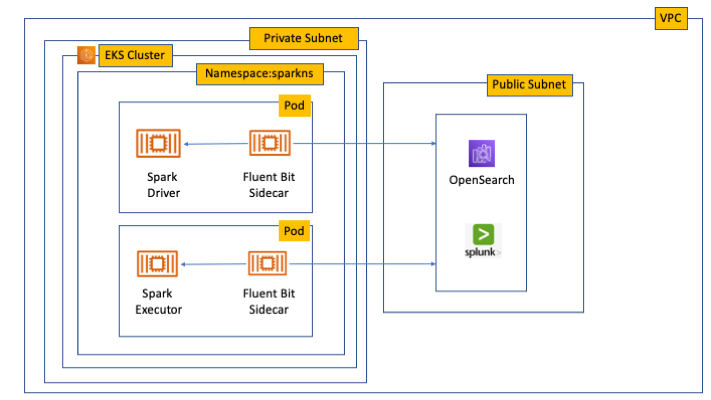
At the core of this architecture are applications composed of microservices (represented by orange boxes) running on Amazon Elastic Kubernetes Service (Amazon EKS). These microservices contain instrumentation that emit telemetry data in the form of metrics, logs, and traces. This data is exported into the OpenTelemetry Collector, which serves as a central vendor agnostic gateway to collect this data uniformly.
In this post, we use an OpenTelemetry demo application as a sample enterprise application. Large enterprise customers typically separate their observability signal data into various stores for scalability, fault isolation, access control, and ease of operation. To aid in these functions, we recommend and use Amazon OpenSearch Ingestion for a serverless, scalable, and fully managed data pipeline. We separate log and trace data and send them to distinct OpenSearch Service domains. The solution also sends the metrics data to Amazon Managed Service for Prometheus.
We use Amazon Managed Grafana as a data visualization and analytics platform to query and visualize this data. We also show how to employ correlations as a valuable tool to gain insights from these signals spread across various data stores.
The following sections outline building this architecture at scale.
Create log and trace OpenSearch Ingestion pipelines
Before setting up the ingestion pipelines, you need to create the necessary AWS Identity and Access Management (IAM) policies and roles. This process involves creating two policies for domain and OSIS access, followed by creating a pipeline role that uses these policies.
Create a policy for ingestion
Complete the following steps to create an IAM policy:
Then, complete the following steps for each OpenSearch Service domain (logs and traces domains).
In OpenSearch Dashboards, go to the Security
Choose Roles and then all_access.
This procedure uses the all_access role for demonstration purposes only. This grants full administrative privileges to the pipeline role, which violates the principle of least privilege and could pose security risks. For production environments, you should create a custom role with minimal permissions required for data ingestion, limit permissions to specific indexes and operations, consider implementing index patterns and time-based access controls, and regularly audit role mappings and permissions. For detailed guidance on creating custom roles with appropriate permissions, refer to Security in Amazon OpenSearch Service.
Choose Mapped users and then Managed mapping.
On the Map user page, under Backend roles, update the backend role with the Amazon Resource Name (ARN) for the role PiplelineRole.
Choose Map.
Create a pipeline for logs
Complete the following steps to create a pipeline for logs:
Define the pipeline configuration by entering the following:
version: "2"
otel-logs-pipeline:
  source:
    otel_logs_source:
      path: "/v1/logs"
  sink:
    - opensearch:
        hosts: ["{OpenSearch_domain_endpoint}"]
        aws:
          sts_role_arn: "arn:aws:iam::{accountId}:role/osi-pipeline-role"
          region: "us-east-1"
          serverless: false
        index: "observability-otel-logs%{yyyy-MM-dd}"

 # To get the values for the placeholders:
 # 1. {OpenSearch_domain_endpoint}: You can find the domain endpoint by navigating to the Amazon Managed Opensearch managed clusters in the AWS Management Console, and then clicking on the domain.
 # After obtaining the necessary values, replace the placeholders in the configuration with the actual values.
Create a pipeline for traces
Complete the following steps to create a pipeline for traces:
Define the pipeline configuration by entering the following:
version: "2"
entry-pipeline:
  source:
    otel_trace_source:
      path: "/v1/traces"
  processor:
    - trace_peer_forwarder:
  sink:
    - pipeline:
        name: "span-pipeline"
    - pipeline:
        name: "service-map-pipeline"
span-pipeline:
  source:
    pipeline:
      name: "entry-pipeline"
  processor:
    - otel_traces:
  sink:
    - opensearch:
        index_type: "trace-analytics-raw"
        hosts: ["{OpenSearch_domain_endpoint}"]
        aws:
          sts_role_arn: "arn:aws:iam::{accountId}:role/osi-pipeline-role"
          region: "us-east-1"
service-map-pipeline:
  source:
    pipeline:
      name: "entry-pipeline"
  processor:
    - service_map:
  sink:
    - opensearch:
        index_type: "trace-analytics-service-map"
        hosts: ["{OpenSearch_domain_endpoint}"]
        aws:
          sts_role_arn: "arn:aws:iam::{accountId}:role/osi-pipeline-role"
          region: "us-east-1"

 # To get the values for the placeholders:
 # 1. {OpenSearch_domain_endpoint}: You can find the domain endpoint by navigating to the Amazon Managed Opensearch managed clusters in the AWS Management Console, and then clicking on the domain.  # 2. {accountId}: This is your AWS account ID. You can find your account ID by clicking on your username in the top-right corner of the AWS Management Console and selecting "My Account" from the dropdown menu.
 # After obtaining the necessary values, replace the placeholders in the configuration with the actual values.
Install the OpenTelemetry demo application in Amazon EKS
Use the EKS cluster you set up earlier along with AWS CloudShell or another tool to complete these steps:
After you have deployed the application, access the frontend application using the load balancer on port 8080. Use your browser to visit http://<LoadBalancerIP>:8080/ to open the source application for OpenTelemetry.
By following these steps, you can successfully install and access demo applications on your EKS cluster.
Configure the OpenTelemetry Collector exporter for logs, traces, and metrics
The OpenTelemetry Collector is a tool that manages the receiving, processing, and exporting of telemetry data from your application to a target repository.
In this step, we send logs and traces to OpenSearch Service and metrics to Amazon Managed Prometheus. The OpenTelemetry Collector also works with popular data repositories like Jaeger and a variety of other open source and commercial platforms. In this section, we include steps to configure the OpenTelemetry Collector in an EKS environment. Then we deploy the demo application and explore the OpenTelemetry exporters using AWS Managed Solutions instead of the open source versions.
Complete the following steps:
Open the otel-collector-config ConfigMap in your preferred editor:
Update the exporters section with the following configuration (provide the appropriate Amazon Managed Service for Prometheus endpoint and OpenSearch Service log ingestion URLs):
With these changes, the OpenTelemetry Collector will send trace data to the OpenSearch Service domain, metrics data to the AWS Managed Service for Prometheus endpoint, and log data to the OpenSearch Service domain.
Configure Amazon Managed Grafana
Before you can visualize your logs and traces, you need to configure OpenSearch Service as a data source in your Amazon Managed Grafana workspace. This configuration is done through the Amazon Managed Grafana console.
Configure the OpenSearch Service data source
Complete the following steps to configure the OpenSearch Service data source:
Select your workspace and choose the workspace URL to access your Grafana instance.
Log in to your Amazon Managed Grafana instance.
From the side menu, choose the configuration (gear) icon.
On the Configuration menu, choose Data Sources.
Choose Add data source.
On the Add data source page, select Amazon Managed Prometheus from the list of available data sources.
In the Name field, enter a descriptive name for the data source.
The AWS Auth Provider and Default Region fields should be automatically populated based on your Amazon Managed Grafana workspace configuration.
In the Workspace field, enter the ID or alias of your Amazon Managed Prometheus workspace.
Choose Save & Test to verify the connection to your Amazon Managed Prometheus workspace.
If the test is successful, you should see a green notification with the message “Data source is working.”
Choose Save to save the data source configuration.
Create correlations in Amazon Managed Grafana
To establish connections between your logs and traces data, you need to set up data correlations in Amazon Managed Grafana. This allows you to navigate seamlessly between related logs and traces. Follow these steps in your Amazon Managed Grafana workspace:
Select your workspace and choose the workspace URL to access your Grafana instance.
In the Amazon Managed Grafana portal, on the Administration menu, choose Plugins and Data, and choose Correlation.
On the Set up the target for the correlation page, under Target, choose your traces data source (OpenSearch Service, for example, otel-traces) from the dropdown list and define the query that will execute when the link is followed. You can use variables to query specific field values. For example, traceId: ${__value.raw}.
On the Set up the target for the correlation page, choose the log data source from the dropdown list, and enter the field name to be linked or correlated with the traces data source in the OpenSearch Service data source. For example, traceID.
Choose Save to complete the correlation configuration.
Repeat the steps to create a correlation between metrics on Prometheus to logs in OpenSearch Service.
Validate results
In Amazon Managed Grafana, using the Prometheus data source, locate the desired instance for correlation. The instance ID will be displayed as a link. Follow the link to open the corresponding log details in a panel on the right side of the page.
With the logs to traces correlation configured, you can access trace information directly from the logs page. Choose traces on the log details panel to view the corresponding trace data.
The following screenshot demonstrates the node graph visualization showing the correlation flow: instance metrics to logs to traces.
Clean up
Remove the infrastructure for this solution when not in use to avoid incurring unnecessary costs.
Conclusion
In this post, we showed how to use correlation as a helpful tool to gain insight into observability data stored in various stores.
Separating logs and traces into dedicated domains provides the following benefits:
Better resource allocation and scaling based on different workload patterns
Independent performance optimization for each data type
Simplified cost tracking and management
Enhanced security control with separate access policies
You can use this solution as a reference to build a scalable observability solution for your enterprise to detect, investigate, and remediate problems faster. This ability, when used along next-generation artificial intelligence and machine learning (AI/ML), helps to not only proactively react but predict and prevent problems before they occur. You can learn more about AI/ML with AWS.
About the Authors
Balaji Mohan is a Senior Delivery Consultant specializing in application and data modernization to the cloud. His business-first approach provides seamless transitions, aligning technology with organizational goals. Using cloud-centered architectures, he delivers scalable, agile, and cost-effective solutions, driving innovation and growth.
Senthil Ramasamy is a Senior Database Consultant at Amazon Web Services. He works with AWS customers to provide guidance and technical assistance on database services, helping them with database migrations to the AWS Cloud and improving the value of their solutions when using AWS.
Muthu Pitchaimani is a Search Specialist with Amazon OpenSearch Service. He builds large-scale search applications and solutions. Muthu is interested in the topics of networking and security, and is based out of Austin, Texas.
Amazon CloudWatch dashboards are customizable pages in the CloudWatch console that you can use to monitor your resources in a single view. This post focuses on deploying a CloudWatch dashboard that you can use to create a customizable monitoring solution for your AWS Network Firewall firewall. It’s designed to provide deeper insights into your firewall’s performance and security events simplifying security monitoring.
Network Firewall is a managed service that you can use to deploy essential network protections to Amazon Virtual Private Clouds (Amazon VPCs). Network Firewall provides comprehensive logs and metrics through CloudWatch, and we’re expanding its capabilities with this CloudWatch dashboard. This enhancement makes it easier to visualize, analyze, and act on the wealth of data generated by your firewall.
This open source solution streamlines network security monitoring with a user-friendly AWS CloudFormation template that quickly deploys a dedicated monitoring dashboard. This solution incorporates a suite of CloudWatch features—basic monitoring metrics, vended logs, Logs Insights queries, Contributor Insights rules, and the dashboard itself—into a centralized view. Preconfigured widgets provide instant insights into critical areas such as top talkers, protocol distributions, and alert log trends, in addition to HTTP and TLS flow analysis. A consolidated view of key metrics and logs enables faster identification of potential security threats or performance issues. With all of this relevant network firewall data in one place, your team can respond more quickly to emerging security events.
In this blog post, we provide an overview of the dashboard and a step-by-step guide to deploy it in your environment.
Solution overview
The CloudWatch dashboard can be deployed in all AWS Regions where Network Firewall is available today, including the AWS GovCloud (US) Regions and China Regions. While the dashboard comes pre-configured, you can quickly adjust queries, time ranges, and refresh intervals to help meet your specific needs. By default, the dashboard queries firewall flow and alert log events over a 3-hour period, impacting the number of log events scanned. Logs Insights and Contributor Insights widgets showcase the top 10 data points by default, but you can enhance results by modifying queries or adjusting the Top Contributors value, though this might lead to increased costs. You can configure the auto-refresh interval of the widgets to get real-time visibility and optimize costs. See the Amazon CloudWatch Pricing guide for up-to-date free and paid tier pricing considerations.
The dashboard, shown in Figure 1, can be deployed using CloudFormation and includes data and analytics from the following sources:
Native CloudWatch metrics from the AWS/NetworkFirewall and AWS/PrivateLinkEndpoints namespaces
CloudWatch Logs Insights queries that analyze Network Firewall flow and alert logs
CloudWatch Contributor Insights rules that aggregate data from Network Firewall flow and alert logs.
Figure 1: CloudWatch dashboard
Walkthrough
In the dashboard, the Logs Insights and Contributor Insights widgets display the top 10 data points by default. You can edit the Insights queries or change the Top Contributors to a larger value to display more results, as shown in Figure 2.
Figure 2: Top Talkers dashboard showing a change to the Top Contributors value
You can also manually refresh the data within a single or multiple widgets, or you can configure the entire dashboard to automatically refresh at a configured time interval as shown in Figure 3. The dashboard won’t automatically refresh the widget data by default.
Figure 3: Configuring the dashboard to automatically refresh
Prerequisites
Deploying the Network Firewall CloudWatch Dashboard is straightforward. You will need the following:
A Network Firewall in your VPC.
Your Network Firewall must be configured to publish firewall flow and alert logs to two different CloudWatch log groups. For example, firewall flow logs are published to /my-firewall-flow-logs and alert logs are published to /my-firewall-alert-logs.
If you haven’t deployed Network Firewall in your VPC, you can use one of the available AWS Network Firewall Deployment Architecture templates to create a firewall. After creating a firewall, configure CloudWatch log groups for the firewall flow and alert logs and configure stateful logging as described previously. Fine-tune your firewall policy and rule configuration and make sure that you’re routing traffic symmetrically through the firewall. With the firewall now in the routed path and publishing metrics and log events, you can proceed with this Network Firewall CloudWatch dashboard template.
Deployment
The Network Firewall dashboard CloudFormation template creates a monitoring dashboard for a single Network Firewall firewall. Make sure that you launch this CloudFormation stack in the same AWS Region and account as the firewall, regardless of whether the firewall is set up centrally or in a distributed manner.
To deploy the dashboard:
Choose Launch Stack for the relevant AWS Region. Make sure that you’re signed in to the appropriate AWS account and Region.
Region: China
Region: Gov Cloud
Region: All other regions supported by AWS Network Firewall
You will be redirected to the Create stack page in the AWS Management Console for CloudFormation. Make sure that you’re in the correct Region and using the correct template. Choose Next. The following are the Regions and their template names:
Figure 4: Make sure that you’re using the correct template
When launching the stack, you will need to enter the following parameters:
Stack name: A descriptive name for this CloudFormation stack. For example, my-firewall-dashboard.
Firewall name: The firewall name as seen in the Amazon VPC console. In the Amazon VPC console, choose Network Firewall in the navigation pane, then choose Firewalls.
Firewall subnets: The firewall subnet IDs to which your firewall endpoints are attached. The firewall subnets can be found on the Firewall details tab of your firewall in the Amazon VPC
Flow log group name: The name of the CloudWatch log group where your firewall flow logs are stored.
Alert log group name: The name of the CloudWatch log group where your firewall alert logs are stored.
Contributor Insights rule state: Enable or disable the Contributor Insights rules (the template defaults to enabled). Disabling will stop the rules from scanning log data and displaying results in the Contributor Insights widgets. After the rules are created, you can change the state of one or more Contributor Insights rules from CloudWatch console by choosing Insights from the navigation pane, and then choosing Contributor Insights.
After the stack reaches CREATE_COMPLETE status, go to the Outputs tab and choose the FirewallDashboardURI link to open the new dashboard in the CloudWatch Dashboards console. It might take a few minutes for the Logs Insights and Contributor Insights widgets to start displaying data. For more details about each widget, see the README. If you don’t have log events matching the query parameters in the widgets, some widgets might not show data points.
Troubleshooting
If you encounter issues during or after deployment, review the following:
Both firewall flow and alert logging are enabled, not just one.
Log group names are entered correctly; incorrect names will cause widgets to point to invalid data.
Correct subnets are selected. Incorrect choices can impact the PrivateLink metrics widgets.
Firewall name is entered correctly. An incorrect name can disrupt metrics widgets, dashboard, and Contributor Insights widget names and break the firewall link.
Cleaning up
You can delete the Network Firewall CloudWatch dashboard and all of the associated resources with a few clicks. Deleting the dashboard will not impact the routing and network traffic inspection performed by the firewall.
Sign in to the CloudFormation console in the Region where you launched the stack and choose Stacks from the navigation pane.
Select the Stack name you chose when launching the stack. For example, my-firewall-dashboard.
Choose Delete.
Conclusion
We encourage you to see for yourself how this new dashboard can enhance your network security management. To get started with the AWS Network Firewall CloudWatch Dashboard, visit our GitHub repository for detailed instructions and the CloudFormation template. For a visual overview of the dashboard and its capabilities, check out our YouTube video.
If you have feedback about this post, submit comments in the Comments section below. If you have questions about this post, contact AWS Support.
Expanding this capability, today we’re launching enhanced observability for your container workloads running on Amazon Elastic Container Service (Amazon ECS). This new capability will help reduce your mean time to detect (MTTD) and mean time to repair (MTTR) for your overall applications, helping prevent issues that could negatively impact your user experience.
Here’s a quick look at Container Insights with enhanced observability for Amazon ECS.
Container Insights with enhanced observability addresses a critical gap in container monitoring. Previously, correlating metrics with logs and events was a time-consuming process, often requiring manual searches and expertise in application architecture. Now, with this capability, CloudWatch and Amazon ECS automatically collect granular performance metrics such as CPU utilization at both the task and container levels while providing visual drill downs enabling easy root-cause analysis.
This new capability enables the following use cases:
Quickly identify root causes by viewing granular resource usage patterns and correlating telemetry data.
Proactively manage your ECS resources using curated dashboards based on AWS best practices.
Track your recent deployments and root causes of your deployment failures with the matching infrastructure anomalies enabling faster issue detection and quicker rollbacks when necessary.
Effortlessly monitor resources across multiple accounts without manual setup. Built-in cross-account support reduces operational overhead with single pane of glass observability.
Integration with other CloudWatch services such as Application Signals and CloudWatch Logs provides a seamless experience to correlate infrastructure with the services running and identify the impacted services.
Using container insights with enhanced observability for Amazon ECS There are two ways to enable Container Insights with enhanced observability:
Cluster-level onboarding – You can enable it for specific clusters individually.
Account-level onboarding – You can also enable it at the account level, which automatically enables observability for all new clusters created in your account. This approach saves time and effort by eliminating the need to manually enable it for each new cluster.
To enable this feature at the account level, I navigate to the Amazon ECS console and select Account settings. Under the CloudWatch Container Insights observability section, I can see it’s currently disabled. I choose Update.
On this page, I find a new option called Container Insights with enhanced observability. I select this option and then choose Save changes.
If I need to enable this capability at the cluster level, I can do so when creating a new cluster.
I can also enable this capability for my existing clusters. To do so, I select Update cluster, and then choose the option.
Once enabled, I can see task-level metrics by navigating to the Metrics tab in my cluster overview console. To access health and performance metrics across my clusters, I can select View Container Insights, which will redirect me to the Container Insights page.
To get a big picture of all my workloads across different clusters, I can navigate to Amazon CloudWatch and then to Container Insights.
This view addresses the challenge of effectively monitoring clusters, services, tasks, and containers by providing a honeycomb visualization that offers an intuitive, high-level summary of cluster health. The dashboard employs a dual-state monitoring approach:
Alarm state (red or green) – Reflects customer-defined thresholds and alerts, allowing teams to configure monitoring based on their specific requirements
Utilization state (dark blue or light blue) – Uses CloudWatch built-in best practices to monitor resource usage patterns across containers. The darker blue indicates clusters operating under higher utilization, enabling teams to proactively identify potential resource constraints before they impact performance
Let’s say there’s an issue in one of my clusters. I can hover over the cluster to display all the alarms created under that cluster at different layers, from the cluster layer down to the container layer.
I also have the option to view all clusters in a list format. The list format is essential for cross-account observability, displaying account IDs and labels for cluster ownership. This helps DevOps engineers quickly identify and collaborate with account owners to resolve potential application issues.
Now, I’d like to explore further. I select my cluster link, which redirects me to the Container Insights detailed dashboard view. Here, I can see a spike in memory utilization for this cluster.
I can dive deeper into container-level details, which help me quickly identify which services are causing this issue.
Another useful feature I found is the Filters option, which helps me conduct more thorough investigations across containers, services, or tasks in this cluster.
If I need to delve deeper into the application logs to understand the root cause of this issue, I can select the task, choose Actions, and choose which logs I would like to view.
On top of using AWS X-Ray traces, I can investigate another two types of logs here. First, I can use performance logs—structured logs containing metric data—to drill down and identify container-level root causes. Second, I examine collected application or container logs . These logs give me detailed insights into application behavior within the container, helping me trace the sequence of events that led to any issues.
In this case, I use application logs.
This streamlines my journey to troubleshoot my application. In this case, the issue is on the downstream calls to third-party applications, which return timeouts.
This integration with Amazon CloudWatch Application Signals provides me with end-to-end visibility, helping me correlate container performance with end-user experience.
When I select datapoints in the graphs, I can see associated traces, which show me all correlated services and their impact. I can also access relevant logs to understand root causes.
Additional things to know Here are a couple of important points to note:
Availability – Container Insights with enhanced observability for ECS is now available in all AWS Regions including the China Regions.
Pricing – Container Insights with enhanced observability for ECS comes with a flat metric pricing, visit the Amazon CloudWatch Pricing page.
Get started today and experience improved observability for your container workloads. Learn more on the Amazon CloudWatch documentation page.
This is a guest post by FINRA (Financial Industry Regulatory Authority). FINRA is dedicated to protecting investors and safeguarding market integrity in a manner that facilitates vibrant capital markets.
FINRA performs big data processing with large volumes of data and workloads with varying instance sizes and types on Amazon EMR. Amazon EMR is a cloud-based big data environment designed to process large amounts of data using open source tools such as Hadoop, Spark, HBase, Flink, Hudi, and Presto.
Monitoring EMR clusters is essential for detecting critical issues with applications, infrastructure, or data in real time. A well-tuned monitoring system helps quickly identify root causes, automate bug fixes, minimize manual actions, and increase productivity. Additionally, observing cluster performance and usage over time helps operations and engineering teams find potential performance bottlenecks and optimization opportunities to scale their clusters, thereby reducing manual actions and improving compliance with service level agreements.
In this post, we talk about our challenges and show how we built an observability framework to provide operational metrics insights for big data processing workloads on Amazon EMR on Amazon Elastic Compute Cloud (Amazon EC2) clusters.
Challenge
In today’s data-driven world, organizations strive to extract valuable insights from large amounts of data. The challenge we faced was finding an efficient way to monitor and observe big data workloads on Amazon EMR due to its complexity. Monitoring and observability for Amazon EMR solutions come with various challenges:
Complexity and scale – EMR clusters often process massive volumes of data across numerous nodes. Monitoring such a complex, distributed system requires handling high data throughput and achieving minimal performance impact. Managing and interpreting the large volume of monitoring data generated by EMR clusters can be overwhelming, making it difficult to identify and troubleshoot issues in a timely manner.
Dynamic environments – EMR clusters are often ephemeral, created and shut down based on workload demands. This dynamism makes it challenging to consistently monitor, collect metrics, and maintain observability over time.
Data variety – Monitoring cluster health and having visibility into clusters to detect bottlenecks, unexpected behavior during processing, data skew, job performance, and so on are crucial. Detailed observability into long-running clusters, nodes, tasks, potential data skews, stuck tasks, performance issues, and job-level metrics (like Spark and JVM) is very critical to understand. Achieving comprehensive observability across these varied data types was difficult.
Resource utilization – EMR clusters consist of various components and services working together, making it challenging to effectively monitor all aspects of the system. Monitoring resource utilization (CPU, memory, disk I/O) across multiple nodes to prevent bottlenecks and inefficiencies is essential but complex, especially in a distributed environment.
Latency and performance metrics –Capturing and analyzing latency and comprehensive performance metrics in real time to identify and resolve issues promptly is critical, but it’s challenging due to the distributed nature of Amazon EMR.
Centralized observability dashboards – Having a single pane of glass for all aspects of EMR cluster metrics, including cluster health, resource utilization, job execution, logs, and security, in order to provide a complete picture of the system’s performance and health, was a challenge.
Alerting and incident management – Setting up effective centralized alerting and notification systems was challenging. Configuring alerts for critical events or performance thresholds requires careful consideration to avoid alert fatigue while making sure important issues are addressed promptly. Responding to incidents from performance slowdowns or disruptions takes time and effort to detect and remediate the issues if proper alerting mechanism is not in place.
Cost management – Lastly, optimizing costs while maintaining effective monitoring is an ongoing challenge. Balancing the need for comprehensive monitoring with cost constraints requires careful planning and optimization strategies to avoid unnecessary expenses while still providing adequate monitoring coverage.
Effective observability for Amazon EMR requires a combination of the right tools, practices, and strategies to address these challenges and provide reliable, efficient, and cost-effective big data processing.
The Ganglia system on Amazon EMR is designed to monitor complete cluster and all nodes’ health, which shows several metrics like Hadoop, Spark, and JVM. When we view the Ganglia web UI in a browser, we see an overview of the EMR cluster’s performance, detailing the load, memory usage, CPU utilization, and network traffic of the cluster through different graphs. However, with Ganglia’s deprecation announced by AWS for higher versions of Amazon EMR, it became important for FINRA to build this solution.
Based on these insights, we completed a successful proof of concept. Next, we built our enterprise central monitoring solution with Managed Prometheus and Managed Grafana to mimic Ganglia-like metrics at FINRA. Managed Prometheus allows for real-time high-volume data collection, which scales the ingestion, storage, and querying of operational metrics as workloads increase or decrease. These metrics are fed to the Managed Grafana workspace for visualizations.
Our solution includes a data ingestion layer for every cluster, with configuration for metrics collection through a custom-built script stored in Amazon Simple Storage Service (Amazon S3). We also installed Managed Prometheus at startup for EC2 instances on Amazon EMR through a bootstrap script. Additionally, application-specific tags are defined in the configuration file to optimize inclusion and collect the specific metrics.
After Managed Prometheus (installed on EMR clusters) collects the metrics, they are sent to a remote Managed Prometheus workspace. Managed Prometheus workspaces are logical and isolated environments dedicated to Managed Prometheus servers that manage specific metrics. They also provide access control for authorizing who or what sends and receives metrics from that workspace. You can create one more workspace by account or application depending on the need, which facilitates better management.
After metrics are collected, we built a mechanism to render them on Managed Grafana dashboards that are then used for consumption through an endpoint. We customized the dashboards for task-level, node-level, and cluster-level metrics so they can be promoted from lower environments to higher environments. We also built several templated dashboards that display node-level metrics like OS-level metrics (CPU, memory, network, disk I/O), HDFS metrics, YARN metrics, Spark metrics, and job-level metrics (Spark and JVM), maximizing the potential for each environment through automated metric aggregation in each account.
We chose a SAML-based authentication option, which allowed us to integrate with existing Active Directory (AD) groups, helping minimize the work needed to manage user access and grant user-based Grafana dashboard access. We arranged three main groups—admins, editors, and viewers—for Grafana user authentication based on user roles.
Through elaborate monitoring automation, these desired metrics are pushed to Amazon CloudWatch. We use CloudWatch for necessary alerting when it exceeds the desired thresholds for each metric.
The following diagram illustrates the solution architecture.
Sample dashboards
The following screenshots showcase example dashboards.
Conclusion
In this post, we shared how FINRA enhanced data-driven decision-making with comprehensive EMR workload observability to optimize performance, maintain reliability, and gain critical insights into big data operations, leading to operational excellence.
FINRA’s solution enabled the operations and engineering teams to use a single pane of glass for monitoring big data workloads and quickly detecting any operational issues. The scalable solution significantly reduced time to resolution and enhanced our overall operational stance. The solution empowered the operations and engineering teams with comprehensive insights into various Amazon EMR metrics like OS levels, Spark, JMX, HDFS, and Yarn, all consolidated in one place. We also extended the solution to use cases such as Amazon Elastic Kubernetes Service (Amazon EKS) clusters, including EMR on EKS clusters and other applications, establishing it as a one-stop system for monitoring metrics across our infrastructure and applications.
About the Authors
Sumalatha Bachu is Senior Director, Technology at FINRA. She manages Big Data Operations which includes managing petabyte-scale data and complex workloads processing in cloud. Additionally, she is an expert in developing Enterprise Application Monitoring and Observability Solutions, Operational Data Analytics, & Machine Learning Model Governance work flows. Outside of work, she enjoys doing yoga, practicing singing, and teaching in her free time.
PremKiran Bejjam is Lead Engineer Consultant at FINRA, specializing in developing resilient and scalable systems. With a keen focus on designing monitoring solutions to enhance infrastructure reliability, he is dedicated to optimizing system performance. Beyond work, he enjoys quality family time and continually seeks out new learning opportunities.
Akhil Chalamalasetty is Director, Market Regulation Technology at FINRA. He is a Big Data subject matter expert specializing in building cutting edge solutions at scale along with optimizing workloads, data, and its processing capabilities. Akhil enjoys sim racing and Formula 1 in his free time.
As organizations increasingly adopt Amazon Q Developer, understanding how developers use it is essential. Diving into specific telemetry events and user-level data clarifies how users interact with Amazon Q Developer, offering insights into feature usage and developer behaviors. This granular view, accessible through logs, is vital for identifying trends, optimizing performance, and enhancing the overall developer experience. This blog is intended to give visibility to key telemetry events logged by Amazon Q Developer and how to explore this data to gain insights.
To help you get started, the following sections will walk through several practical examples that showcase how to extract meaningful insights from AWS CloudTrail. By reviewing the logs, organizations can track usage patterns, identify top users, and empower them to train and mentor other developers, ultimately fostering broader adoption and engagement across teams.
Although the examples here focus on Amazon Athena for querying logs, the methods can be adapted to integrate with other tools like Splunk or Datadog for further analysis. Through this exploration, readers will learn how to query the log data to understand better how Amazon Q Developer is used within your organization.
Solution Overview
This solution leverages Amazon Q Developer’s logs from the Integrated Development Environment (IDE) and terminal, captured in AWS CloudTrail. The logs will be queried directly using Amazon Athena from Amazon Simple Storage Service (Amazon S3) to analyze feature usage, such as in-line code suggestions, chat interactions, and security scanning events.
Analyzing Telemetry Events in Amazon Q Developer
Amazon Athena is used to query the CloudTrail logs directly to analyze this data. By utilizing Athena, queries can be run on existing CloudTrail records, making it simple to extract insights from the data in its current format.
Ensuring CloudTrail is set up to log the data events.
Navigate to the AWS CloudTrail Console.
Edit an Existing Trail:
If you have a trail, verify it is configured to log data events for Amazon CodeWhisperer.
Note: As of 4/30/24, CodeWhisperer has been renamed to Amazon Q Developer. All the functionality previously provided by CodeWhisperer is now part of Amazon Q Developer. However, for consistency, the original API names have been retained.
Click on your existing trail in CloudTrail. Find the Data Events section and click edit.
For CodeWhisperer:
Data event type: CodeWhisperer
Log selector template: Log all events
Save your changes.
Note your “Trail log location.” This S3 bucket will be used in our Athena setup.
If you don’t have an existing trail, follow the instructions in the AWS CloudTrail User Guide to set up a new trail.
Below is a screenshot of the data events addition:
Steps to Create an Athena Table from CloudTrail Logs: This step aims to turn CloudTrail events into a queryable Athena table.
1. Navigate to the AWS Management Console > Athena > Editor.
2. Click on the plus to create a query tab.
3. Run the following query to create a database and table. Note to update the location to your S3 bucket.
-- Step 1: Create a new database (if it doesn't exist)
CREATE DATABASE IF NOT EXISTS amazon_q_metrics;

-- Step 2: Create the external table explicitly within the new database
CREATE EXTERNAL TABLE amazon_q_metrics.cloudtrail_logs (

    userIdentity STRUCT<
        accountId: STRING,
        onBehalfOf: STRUCT<
            userId: STRING,
            identityStoreArn: STRING
        >
    >,
    eventTime STRING,
    eventSource STRING,
    eventName STRING,
    requestParameters STRING,
    requestId STRING,
    eventId STRING,
    resources ARRAY<STRUCT<
        arn: STRING,
        accountId: STRING,
        type: STRING
    >>,
    recipientAccountId STRING

)
ROW FORMAT SERDE 'org.apache.hive.hcatalog.data.JsonSerDe'
STORED AS INPUTFORMAT 'com.amazon.emr.cloudtrail.CloudTrailInputFormat'
OUTPUTFORMAT 'org.apache.hadoop.hive.ql.io.HiveIgnoreKeyTextOutputFormat'
LOCATION 's3://{Insert Bucket Name from CloudTrail}/'
TBLPROPERTIES ('classification'='cloudtrail');
4. Click Run
5. Run a quick query to view the data.
SELECT
    eventTime,
    userIdentity.onBehalfOf.userId AS user_id,
    eventName,
    requestParameters
FROM
    amazon_q_metrics.cloudtrail_logs AS logs
WHERE
    eventName = 'SendTelemetryEvent'
LIMIT 10;
In this section, the significance of the telemetry events captured in the requestParameters field will be explained. The query begins by displaying key fields and their data, offering insights into how users interact with various features of Amazon Q Developer.
Query Breakdown:
eventTime: This field captures the time the event was recorded, providing insights into when specific user interactions took place.
userIdentity.onBehalfOf.userId: This extracts the userId of the user. This is critical for attributing interactions to the correct user, which will be covered in more detail later in the blog.
eventName: The query is filtered on SendTelemetryEvent. Telemetry events are triggered when the user interacts with particular features or when a developer uses the service.
requestParameters: The requestParameters field is crucial because it holds the details of the telemetry events. This field contains a rich set of information depending on the type of interaction and feature the developer uses, which programming languages are used, completion types, or code modifications.
In the context of the SendTelemetryEvent, various telemetry events are captured in the requestParameters field of CloudTrail logs. These events provide insights into user interactions, overall usage, and the effectiveness of Amazon Q Developer’s suggestions. Here are the key telemetry events along with their descriptions:
UserTriggerDecisionEvent
Description: This event is triggered when a user interacts with a suggestion made by Amazon Q Developer. It captures whether the suggestion was accepted or rejected, along with relevant metadata.
Key Fields:
completionType: Whether the completion was a block or a line.
suggestionState: Whether the user accepted, rejected, or discarded the suggestion.
programmingLanguage: The programming language associated with the suggestion.
generatedLine: The number of lines generated by the suggestion.
CodeScanEvent
Description: This event is logged when a code scan is performed. It helps track the scope and result of the scan, providing insights into security and code quality checks.
Key Fields:
codeAnalysisScope: Whether the scan was performed at the file level or the project level.
programmingLanguage: The language being scanned.
CodeScanRemediationsEvent
Description: This event captures user interactions with Amazon Q Developer’s remediation suggestions, such as applying fixes or viewing issue details.
Key Fields:
CodeScanRemediationsEventType: The type of remediation action taken (e.g., viewing details or applying a fix).
includesFix: A boolean indicating whether the user applied a fix.
ChatAddMessageEvent
Description: This event is triggered when a new message is added to an ongoing chat conversation. It captures the user’s intent which refers to the purpose or goal the user is trying to achieve with the chat message. The intent can include various actions, such as suggesting alternate implementations of the code, applying common best practices, improving the quality or performance of the code.
Key Fields:
conversationId: The unique identifier for the conversation.
messageId: The unique identifier for the chat message.
userIntent: The user’s intent, such as improving code or explaining code.
programmingLanguage: The language related to the chat message.
ChatInteractWithMessageEvent
Description: This event captures when users interact with chat messages, such as copying code snippets, clicking links, or hovering over references.
Key Fields:
interactionType: The type of interaction (e.g., copy, hover, click).
interactionTarget: The target of the interaction (e.g., a code snippet or a link).
acceptedCharacterCount: The number of characters from the message that were accepted.
acceptedSnippetHasReference: A boolean indicating if the accepted snippet included a reference.
TerminalUserInteractionEvent
Description: This event logs user interactions with terminal commands or completions in the terminal environment.
Key Fields:
terminalUserInteractionEventType: The type of interaction (e.g., terminal translation or code completion).
isCompletionAccepted: A boolean indicating whether the completion was accepted by the user.
terminal: The terminal environment in which the interaction occurred.
shell: The shell used for the interaction (e.g., Bash, Zsh).
Telemetry events are key to understanding how users engage with Amazon Q Developer. They track interactions such as code completion, security scans, and chat-based suggestions. Analyzing the data in the requestParameters field helps reveal usage patterns and behaviors that offer valuable insights.
By exploring events such as UserTriggerDecisionEvent, ChatAddMessageEvent, TerminalUserInteractionEvent, and others in the schema, organizations can assess the effectiveness of Amazon Q Developer and identify areas for improvement.
Example Queries for Analyzing Developer Engagement
To gain deeper insights into how developers interact with Amazon Q Developer, the following queries can help analyze key telemetry data from CloudTrail logs. These queries track in-line code suggestions, chat interactions, and code-scanning activities. By running these queries, you can uncover valuable metrics such as the frequency of accepted suggestions, the types of chat interactions, and the programming languages most frequently scanned. This analysis helps paint a clear picture of developer engagement and usage patterns, guiding efforts to enhance productivity.
These four examples only cover a sample set of the available telemetry events, but they serve as a starting point for further exploration of Amazon Q Developer’s capabilities.
SELECT
    eventTime,
    userIdentity.onBehalfOf.userId AS user_id,
    eventName,
    json_extract_scalar(requestParameters, '$.telemetryEvent.userTriggerDecisionEvent.suggestionState') AS suggestionState,
    json_extract_scalar(requestParameters, '$.telemetryEvent.userTriggerDecisionEvent.completionType') AS completionType
FROM
    amazon_q_metrics.cloudtrail_logs
WHERE
    eventName = 'SendTelemetryEvent'
    AND json_extract(requestParameters, '$.telemetryEvent.userTriggerDecisionEvent') IS NOT NULL
    AND json_extract_scalar(requestParameters, '$.telemetryEvent.userTriggerDecisionEvent.suggestionState') = 'ACCEPT';
Use Case:This use case focuses on how developers interact with in-line code suggestions by analyzing accepted snippets. It helps identify which users are accepting suggestions, the type of snippets being accepted (blocks or lines), and the programming languages involved. Understanding these patterns can reveal how well Amazon Q Developer aligns with the developers’ expectations.
Query Explanation: The query retrieves the event time, user ID, event name, suggestion state (filtered to show only ACCEPT), and completion type. TotalGeneratedLinesBlockAccept and totalGeneratedLinesLineAccept or discarded suggestions are not included, but this gives an idea of the developers using the service for in-line code suggestions and the lines or blocks they have accepted. Additionally, the programming language field can be extracted to see which languages are used during these interactions.
Query 2: Analyzing Chat Interactions
SELECT
    userIdentity.onBehalfOf.userId AS userId,
    json_extract_scalar(requestParameters, '$.telemetryEvent.chatInteractWithMessageEvent.interactionType') AS interactionType,
    COUNT(*) AS eventCount
FROM
    amazon_q_metrics.cloudtrail_logs
WHERE
    eventName = 'SendTelemetryEvent'
    AND json_extract(requestParameters, '$.telemetryEvent.chatInteractWithMessageEvent') IS NOT NULL
GROUP BY
    userIdentity.onBehalfOf.userId,
    json_extract_scalar(requestParameters, '$.telemetryEvent.chatInteractWithMessageEvent.interactionType')
ORDER BY
    eventCount DESC;
Use Case: This use case looks at how developers use chat options like upvoting, downvoting, and copying code snippets. Understanding the chat usage patterns shows which interactions are most used and how developers engage with Amazon Q Developer chat. As an organization, this insight can help support other developers in successfully leveraging this feature.
Query Explanation: The query provides insights into chat interactions within Amazon Q Developer by retrieving user IDs, interaction types, and event counts. This query aggregates data based on the interactionType field within chatInteractWithMessageEvent, showcasing various user actions such as UPVOTE, DOWNVOTE, INSERT_AT_CURSOR, COPY_SNIPPET, COPY, CLICK_LINK, CLICK_BODY_LINK, CLICK_FOLLOW_UP, and HOVER_REFERENCE.
This analysis highlights how users engage with the chat feature and the interactions, offering a view of interaction patterns. By focusing on the interactionType field, you can better understand how developers interact with the chat feature of Amazon Q Developer.
Query 3: Analyzing Code Scanning Jobs Across Programming Languages
SELECT
    userIdentity.onBehalfOf.userId AS userId,
    json_extract_scalar(requestParameters, '$.telemetryEvent.codeScanEvent.programmingLanguage.languageName') AS programmingLanguage,
    COUNT(json_extract_scalar(requestParameters, '$.telemetryEvent.codeScanEvent.codeScanJobId')) AS jobCount
FROM
    amazon_q_metrics.cloudtrail_logs
WHERE
    eventName = 'SendTelemetryEvent'
    AND json_extract(requestParameters, '$.telemetryEvent.codeScanEvent') IS NOT NULL
GROUP BY
    userIdentity.onBehalfOf.userId,
    json_extract_scalar(requestParameters, '$.telemetryEvent.codeScanEvent.programmingLanguage.languageName')
ORDER BY
    jobCount DESC;
Use Case: Amazon Q Developer includes security scanning, and this section helps determine how the security scanning feature is being used across different users and programming languages within the organization. Understanding these trends provides valuable insights into which users actively perform security scans and the specific languages targeted for these scans.
Query Explanation: The query provides insights into the distribution of code scanning jobs across different programming languages in Amazon Q Developer. It retrieves user IDs and the count of code-scanning jobs by programming language. This analysis focuses on the CodeScanEvent, aggregating data to show the total number of jobs executed per language.
By summing up the number of code scanning jobs per programming language, this query helps to understand which languages are most frequently analyzed. It provides a view of how users are leveraging the code-scanning feature. This can be useful for identifying trends in language usage and optimizing code-scanning practices.
Query 4: Analyzing User Activity across features.
SELECT
    userIdentity.onBehalfOf.userId AS user_id,
    COUNT(DISTINCT CASE
        WHEN json_extract(requestParameters, '$.telemetryEvent.userTriggerDecisionEvent') IS NOT NULL
        THEN eventId END) AS inline_suggestions_count,
    COUNT(DISTINCT CASE
        WHEN json_extract(requestParameters, '$.telemetryEvent.chatInteractWithMessageEvent') IS NOT NULL
        THEN eventId END) AS chat_interactions_count,
    COUNT(DISTINCT CASE
        WHEN json_extract(requestParameters, '$.telemetryEvent.codeScanEvent') IS NOT NULL
        THEN eventId END) AS security_scans_count,
    COUNT(DISTINCT CASE
        WHEN json_extract(requestParameters, '$.telemetryEvent.terminalUserInteractionEvent') IS NOT NULL
        THEN eventId END) AS terminal_interactions_count
FROM
    amazon_q_metrics.cloudtrail_logs
WHERE
    eventName = 'SendTelemetryEvent'
GROUP BY
    userIdentity.onBehalfOf.userId
Use Case:This use case looks at how developers use Amazon Q Developer across different features: in-line code suggestions, chat interactions, security scans, and terminal interactions. By tracking usage, organizations can see overall engagement and identify areas where developers may need more support or training. This helps optimize the use of Amazon Q Developer and helps teams get the most out of the tool.
Query Explanation: Let’s take the other events from the prior queries and additional events to get more detail overall and tie it all together. This expanded query provides a comprehensive view of user activity within Amazon Q Developer by tracking the number of in-line code suggestions, chat interactions, security scans, and terminal interactions performed by each user. By analyzing these events, organizations can gain a better understanding of how developers are using these key features.
By summing up the interactions for each feature, this query helps identify which users are most active in each category, offering insights into usage patterns and areas where additional training or support may be needed.
Enhancing Metrics with Display Names and Usernames
The previous queries had userid as a field; however, many customers would prefer to see a user alias (such as username or display name). The following section illustrates enhancing these metrics by augmenting user IDs with display names and usernames from the AWS IAM Identity Center. This will provide more human-readable user names.
In this example, the export is run locally to enhance user metrics with IAM Identity Center for simplicity. This method works well for demonstrating how to access and work with the data, but it provides a static snapshot of the users at the time of export. In a production environment, an automated solution would be preferable to capture newly added users continuously. For the purposes of this blog, this straightforward approach is used to focus on data access.
To proceed, install Python 3.8+ and Boto3, and configure AWS credentials via the CLI. Then, run the following Python script locally to export the data:
import boto3, csv
# replace this with the region of your IDC instance
RegionName='us-east-1'
# client creation
idstoreclient = boto3.client('identitystore', RegionName)
ssoadminclient = boto3.client('sso-admin', RegionName)

Instances= (ssoadminclient.list_instances()).get('Instances')
InstanceARN=Instances[0].get('InstanceArn')
IdentityStoreId=Instances[0].get('IdentityStoreId')

# query
UserDigestList = []
ListUserResponse = idstoreclient.list_users(IdentityStoreId=IdentityStoreId)
UserDigestList.extend([[user['DisplayName'], user['UserName'], user['UserId']] for user in ListUserResponse['Users']])
NextToken = None
if 'NextToken' in ListUserResponse.keys(): NextToken = ListUserResponse['NextToken']
while NextToken is not None:
    ListUserResponse = idstoreclient.list_users(IdentityStoreId=IdentityStoreId, NextToken=NextToken)
    UserDigestList.extend([[user['DisplayName'], user['UserName'], user['UserId']] for user in ListUserResponse['Users']])
    if 'NextToken' in ListUserResponse.keys(): NextToken = ListUserResponse['NextToken']
    else: NextToken = None

# write the query results to IDCUserInfo.csv
with open('IDCUserInfo.csv', 'w') as CSVFile:
    CSVWriter = csv.writer(CSVFile, quoting=csv.QUOTE_ALL)
    HeaderRow = ['DisplayName', 'UserName', 'UserId']
    CSVWriter.writerow(HeaderRow)
    for UserRow in UserDigestList:
        CSVWriter.writerow(UserRow)
This script will query the IAM Identity Center for all users and write the results to a CSV file, including DisplayName, UserName, and UserId. After generating the CSV file, upload it to an S3 bucket. Please make note of this S3 location.
Steps to Create an Athena Table from the above CSV output: Create a table in Athena to join the existing table with the user details.
1. Navigate to the AWS Management Console > Athena > Editor.
2. Click on the plus to create a query tab.
3. Run the following query to create our table. Note to update the location to your S3 bucket.
CREATE EXTERNAL TABLE amazon_q_metrics.user_data (
    DisplayName STRING,
    UserName STRING,
    UserId STRING
)
ROW FORMAT SERDE 'org.apache.hadoop.hive.serde2.OpenCSVSerde'
WITH SERDEPROPERTIES (
   'separatorChar' = ',',
   'quoteChar'     = '"'
)
STORED AS TEXTFILE
LOCATION 's3://{Update to your S3 object location}/'  -- Path containing CSV file
TBLPROPERTIES ('skip.header.line.count'='1');
4. Click Run
5. Now, let’s run a quick query to verify the data in the new table.
SELECT * FROM amazon_q_metrics.user_data limit 10;
The first query creates an external table in Athena from user data stored in a CSV file in S3. The user_data table has three fields: DisplayName, UserName, and UserId. To specify the correct parsing of the CSV, separatorChar is specified as a comma and quoteChar as a double quote. Additionally, the TBLPROPERTIES (‘skip.header.line.count’=’1’) flag skips the header row in the CSV file, ensuring that column names aren’t treated as data.
The user_data table holds key details: DisplayName (full name), UserName (username), and UserId (unique identifier). This table will be joined with the cloudtrail_q_metrics table using the userId field from the onBehalfOf struct, enriching the interaction logs with human-readable user names and display names instead of user IDs.
In the previous analysis of in-line code suggestions, the focus was on retrieving key metrics related to user interactions with Amazon Q Developer. The query below follows a similar structure but now includes a join with the user_data table to enrich insights with additional user details such as DisplayName and Username.
To include a join with the user_data table in the query, it is necessary to define a shared key between the cloudtrail_logs_amazon_q and user_data tables. For this example, user_id will be used.
SELECT
    logs.eventTime,
    user_data.displayname,  -- Additional field from user_data table
    user_data.username,     -- Additional field from user_data table
    json_extract_scalar(logs.requestParameters, '$.telemetryEvent.userTriggerDecisionEvent.suggestionState') AS suggestionState,
    json_extract_scalar(logs.requestParameters, '$.telemetryEvent.userTriggerDecisionEvent.completionType') AS completionType
FROM
    amazon_q_metrics.cloudtrail_logs AS logs  -- Specified database for cloudtrail_logs
JOIN
    amazon_q_metrics.user_data  -- Specified database for user_data
ON
    logs.userIdentity.onBehalfOf.userId = user_data.userid
WHERE
    logs.eventName = 'SendTelemetryEvent'
    AND json_extract_scalar(logs.requestParameters, '$.telemetryEvent.userTriggerDecisionEvent.suggestionState') = 'ACCEPT';
This approach allows for a deeper analysis by integrating user-specific information with the telemetry data, helping you better understand how different user roles interact with the in-line suggestions and other features of Amazon Q Developer.
Cleanup
If you have been following along with this workflow, it is important to clean up the resources to avoid unnecessary charges. You can perform the cleanup by running the following query in the Amazon Athena console:
-- Step 1: Drop the tables
DROP TABLE IF EXISTS amazon_q_metrics.cloudtrail_logs;
DROP TABLE IF EXISTS amazon_q_metrics.user_data;

-- Step 2: Drop the database after the tables are removed
DROP DATABASE IF EXISTS amazon_q_metrics CASCADE;
This query removes both the cloudtrail_logs and user_data tables, followed by the amazon_q_metrics database.
Remove the S3 objects used to store the CloudTrail logs and user data by navigating to the S3 console, selecting the relevant buckets or objects, and choosing “Delete.”
If a new CloudTrail trail was created, consider deleting it to stop further logging. For instructions, see Deleting a Trail. If an existing trail was used, remove the CodeWhisperer data events to prevent continued logging of those events.
Conclusion
By tapping into Amazon Q Developer’s logging capabilities, organizations can unlock detailed insights that drive better decision-making and boost developer productivity. The ability to analyze user-level interactions provides a deeper understanding of how the service is used.
Now that you have these insights, the next step is leveraging them to drive improvements. For example, organizations can use this data to identify opportunities for Proof of Concepts (PoCs) and pilot programs that further demonstrate the value of Amazon Q Developer. By focusing on areas where engagement is high, you can support the most engaged developers as champions to advocate for the tool across the organization, driving broader adoption.
The true potential of these insights lies in the “art of the possible.” With the data provided, it is up to you to explore how to query or visualize it further. Whether you’re examining metrics for in-line code suggestions, interactions, or security scanning, this foundational analysis is just the beginning.
As Amazon Q Developer continues to evolve, staying updated with emerging telemetry events is crucial for maintaining visibility into the available metrics. You can do this by regularly visiting the official Amazon Q Developer documentation and the Amazon Q Developer’s Changelog to stay up-to-date latest information and insights.
Amazon EMR Serverless allows you to run open source big data frameworks such as Apache Spark and Apache Hive without managing clusters and servers. With EMR Serverless, you can run analytics workloads at any scale with automatic scaling that resizes resources in seconds to meet changing data volumes and processing requirements.
We have launched job worker metrics in Amazon CloudWatch for EMR Serverless. This feature allows you to monitor vCPUs, memory, ephemeral storage, and disk I/O allocation and usage metrics at an aggregate worker level for your Spark and Hive jobs.
This post is part of a series about EMR Serverless observability. In this post, we discuss how to use these CloudWatch metrics to monitor EMR Serverless workers in near real time.
CloudWatch metrics for EMR Serverless
At the per-Spark job level, EMR Serverless emits the following new metrics to CloudWatch for both driver and executors. These metrics provide granular insights into job performance, bottlenecks, and resource utilization.
WorkerCpuAllocated
The total numbers of vCPU cores allocated for workers in a job run
WorkerCpuUsed
The total numbers of vCPU cores utilized by workers in a job run
WorkerMemoryAllocated
The total memory in GB allocated for workers in a job run
WorkerMemoryUsed
The total memory in GB utilized by workers in a job run
WorkerEphemeralStorageAllocated
The number of bytes of ephemeral storage allocated for workers in a job run
WorkerEphemeralStorageUsed
The number of bytes of ephemeral storage used by workers in a job run
WorkerStorageReadBytes
The number of bytes read from storage by workers in a job run
WorkerStorageWriteBytes
The number of bytes written to storage from workers in a job run
The following are the benefits of monitoring your EMR Serverless jobs with CloudWatch:
Optimize resource utilization – You can gain insights into resource utilization patterns and optimize your EMR Serverless configurations for better efficiency and cost savings. For example, underutilization of vCPUs or memory can reveal resource wastage, allowing you to optimize worker sizes to achieve potential cost savings.
Diagnose common errors – You can identify root causes and mitigation for common errors without log diving. For example, you can monitor the usage of ephemeral storage and mitigate disk bottlenecks by preemptively allocating more storage per worker.
Gain near real-time insights – CloudWatch offers near real-time monitoring capabilities, allowing you to track the performance of your EMR Serverless jobs as and when they are running, for quick detection of any anomalies or performance issues.
Configure alerts and notifications – CloudWatch enables you to set up alarms using Amazon Simple Notification Service (Amazon SNS) based on predefined thresholds, allowing you to receive notifications through email or text message when specific metrics reach critical levels.
Conduct historical analysis – CloudWatch stores historical data, allowing you to analyze trends over time, identify patterns, and make informed decisions for capacity planning and workload optimization.
Solution overview
To further enhance this observability experience, we have created a solution that gathers all these metrics on a single CloudWatch dashboard for an EMR Serverless application. You need to launch one AWS CloudFormation template per EMR Serverless application. You can monitor all the jobs submitted to a single EMR Serverless application using the same CloudWatch dashboard. To learn more about this dashboard and deploy this solution into your own account, refer to the EMR Serverless CloudWatch Dashboard GitHub repository.
In the following sections, we walk you through how you can use this dashboard to perform the following actions:
Optimize your resource utilization to save costs without impacting job performance
Diagnose failures due to common errors without the need for log diving and resolve those errors optimally
You need to submit all the jobs in this post to the same EMR Serverless application. If you want to monitor a different application, you can deploy this template for your own EMR Serverless application ID.
Optimize resource utilization
When running Spark jobs, you often start with the default configurations. It can be challenging to optimize your workload without any visibility into actual resource utilization. Some of the most common configurations that we’ve seen customers adjust are spark.driver.cores, spark.driver.memory, spark.executor.cores, and spark.executors.memory.
To illustrate how the newly added CloudWatch dashboard worker-level metrics can help you fine-tune your job configurations for better price-performance and enhanced resource utilization, let’s run the following Spark job, which uses the NOAA Integrated Surface Database (ISD) dataset to run some transformations and aggregations.
Use the following command to run this job on EMR Serverless. Provide your Amazon Simple Storage Service (Amazon S3) bucket and EMR Serverless application ID for which you launched the CloudFormation template. Make sure to use the same application ID to submit all the sample jobs in this post. Additionally, provide an AWS Identity and Access Management (IAM) runtime role.
Now let’s check the executor vCPUs and memory from the CloudWatch dashboard.
This job was submitted with default EMR Serverless Spark configurations. From the Executor CPU Allocated metric in the preceding screenshot, the job was allocated 396 vCPUs in total (99 executors * 4 vCPUs per executor). However, the job only used a maximum of 110 vCPUs based on Executor CPU Used. This indicates oversubscription of vCPU resources. Similarly, the job was allocated 1,584 GB memory in total based on Executor Memory Allocated. However, from the Executor Memory Used metric, we see that the job only used 176 GB of memory during the job, indicating memory oversubscription.
Now let’s rerun this job with the following adjusted configurations.
Let’s check the executor metrics from the CloudWatch dashboard again for this job run.
In the second job, we see lower allocation of both vCPUs (396 vs. 60) and memory (1,584 GB vs. 120 GB) as expected, resulting in better utilization of resources. The original job ran for 4 minutes, 41 seconds. The second job took 4 minutes, 54 seconds. This reconfiguration has resulted in 79% lower cost savings without affecting the job performance.
You can use these metrics to further optimize your job by increasing or decreasing the number of workers or the allocated resources.
Diagnose and resolve job failures
Using the CloudWatch dashboard, you can diagnose job failures due to issues related to CPU, memory, and storage such as out of memory or no space left on the device. This enables you to identify and resolve common errors quickly without having to check the logs or navigate through Spark History Server. Additionally, because you can check the resource utilization from the dashboard, you can fine-tune the configurations by increasing the required resources only as much as needed instead of oversubscribing to the resources, which further saves costs.
Driver errors
To illustrate this use case, let’s run the following Spark job, which creates a large Spark data frame with a few million rows. Typically, this operation is done by the Spark driver. While submitting the job, we also configure spark.rpc.message.maxSize, because it’s required for task serialization of data frames with a large number of columns.
After a few minutes, the job failed with the error message “Encountered errors when releasing containers,” as seen in the Job details section.
When encountering non-descriptive error messages, it becomes crucial to investigate further by examining the driver and executor logs to troubleshoot further. But before further log diving, let’s first check the CloudWatch dashboard, specifically the driver metrics, because releasing containers is generally performed by the driver.
We can see that the Driver CPU Used and Driver Storage Used are well within their respective allocated values. However, upon checking Driver Memory Allocated and Driver Memory Used, we can see that the driver was using all of the 16 GB memory allocated to it. By default, EMR Serverless drivers are assigned 16 GB memory.
Let’s rerun the job with more driver memory allocated. Let’s set driver memory to 27 GB as the starting point, because spark.driver.memory + spark.driver.memoryOverhead should be less than 30 GB for the default worker type. park.rpc.messsage.maxSize will be unchanged.
The job succeeded this time around. Let’s check the CloudWatch dashboard to observe driver memory utilization.
As we can see, the allocated memory is now 30 GB, but the actual driver memory utilization didn’t exceed 21 GB during the job run. Therefore, we can further optimize costs here by reducing the value of spark.driver.memory. We reran the same job with spark.driver.memory set to 22 GB, and the job still succeeded with better driver memory utilization.
Executor errors
Using CloudWatch for observability is ideal for diagnosing driver-related issues because there is only one driver per job and driver resources used is the actual resource usage of the single driver. On the other hand, executor metrics are aggregated across all the workers. However, you can use this dashboard to provide only an adequate amount of resources to make your job succeed, thereby avoiding oversubscription of resources.
To illustrate, let’s run the following Spark job, which simulates uniform disk over-utilization across all workers by processing very large NOAA datasets from several years. This job also transiently caches a very large data frame on disk.
After a few minutes, we can see that the job failed with “No space left on device” error in the Job details section, which indicates that some of the workers have run out of disk space.
Checking the Running Executors metric from the dashboard, we can identify that there were 99 executor workers running. Each worker comes with 20 GB storage by default.
Because this is a Spark task failure, let’s check the Executor Storage Allocated and Executor Storage Used metrics from the dashboard (because the driver won’t run any tasks).
As we can see, the 99 executors have used up a total of 1,940 GB from the total allocated executor storage of 2,126 GB. This includes both the data shuffled by the executors and the storage used for caching the data frame. We don’t see the full 2,126 GB being utilized from this graph because there might be a few executors out of the 99 executors that weren’t holding much data when the job failed (before these executors could start processing tasks and store the data frame chunks).
Let’s rerun the same job but with increased executor disk size using the parameter spark.emr-serverless.executor.disk. Let’s try with 40 GB disk per executor as a starting point.
This time, the job ran successfully. Let’s check the Executor Storage Allocated and Executor Storage Used metrics.
Executor Storage Allocated is now 4,251 GB because we’ve doubled the value of spark.emr-serverless.executor.disk. Although there is now twice as much aggregated executors’ storage, the job still used only a maximum of 1,940 GB out of 4,251 GB. This indicates that our executors were likely running out of disk space only by a few GBs. Therefore, we can try to set spark.emr-serverless.executor.disk to an even lower value like 25 GB or 30 GB instead of 40 GB to save storage costs as we did in the previous scenario. In addition, you can monitor Executor Storage Read Bytes and Executor Storage Write Bytes to see if your job is I/O intensive. In this case, you can use the Shuffle-optimized disks feature of EMR Serverless to further enhance your job’s I/O performance.
The dashboard is also useful to capture information about transient storage used while caching or persisting the data frames, including spill-to-disk scenarios. The Storage tab of Spark History Server records any caching activities, as seen in the following screenshot. However, this data will be lost from Spark History Server after the cache is evicted or when the job finishes. Therefore, Executor Storage Used can be used to do an analysis of a failed job run due to transient storage issues.
In this particular example, the data was evenly distributed among the executors. However, if you have a data skew (for, example only 1–2 executors out of 99 process the most amount of data, and as a result, your job runs out of disk space), the CloudWatch dashboard won’t accurately capture this scenario because the storage data is aggregated across all the executors for a job. For diagnosing issues at the individual executor level, we need to track per-executor-level metrics. We explore more advanced examples of how per-worker-level metrics can help you identify, mitigate, and resolve hard-to-find issues through EMR Serverless integration with Amazon Managed Service for Prometheus.
Conclusion
In this post, you learned how to effectively manage and optimize your EMR Serverless application using a single CloudWatch dashboard with enhanced EMR Serverless metrics. These metrics are available in all AWS Regions where EMR Serverless is available. For more details about this feature, refer to Job-level monitoring.
About the Authors
Kashif Khan is a Sr. Analytics Specialist Solutions Architect at AWS, specializing in big data services like Amazon EMR, AWS Lake Formation, AWS Glue, Amazon Athena, and Amazon DataZone. With over a decade of experience in the big data domain, he possesses extensive expertise in architecting scalable and robust solutions. His role involves providing architectural guidance and collaborating closely with customers to design tailored solutions using AWS analytics services to unlock the full potential of their data.
Veena Vasudevan is a Principal Partner Solutions Architect and Data & AI specialist at AWS. She helps customers and partners build highly optimized, scalable, and secure solutions; modernize their architectures; and migrate their big data, analytics, and AI/ML workloads to AWS.
Maximizing the value from Enterprise Software tools requires an understanding of who and how users interact with those tools. As we have worked with builders rolling out Amazon CodeWhisperer to their enterprises, identifying usage patterns has been critical.
This blog post is a result of that work, builds on Introducing Amazon CodeWhisperer Dashboard blog and Amazon CloudWatch metrics and enables customers to build dashboards to support their rollouts. Note that these features are only available in CodeWhisperer Professional plan.
Organizations have leveraged the existing Amazon CodeWhisperer Dashboard to gain insights into developer usage. This blog explores how we can supplement the existing dashboard with detailed user analytics. Identifying leading contributors has accelerated tool usage and adoption within organizations. Acknowledging and incentivizing adopters can accelerate a broader adoption.
The architecture diagram outlines a streamlined process for tracking and analyzing Amazon CodeWhisperer usage events. It begins with logging these events in CodeWhisperer and AWS CloudTrail and then forwarding them to Amazon CloudWatch Logs. Configuring AWS CloudTrail involves using Amazon S3 for storage and AWS Key Management Service (KMS) for log encryption. An AWS Lambda function analyzes the logs, extracting information about user activity. This blog also introduces a AWS CloudFormation template that simplifies the setup process, including creating the CloudTrail with an S3 bucket KMS key and the Lambda function. The template also configures AWS IAM permissions, ensuring the Lambda function has access rights to interact with other AWS services.
Configuring CloudTrail for CodeWhisperer User Tracking
This section details the process for monitoring user interactions while using Amazon CodeWhisperer. The aim is to utilize AWS CloudTrail to record instances where users receive code suggestions from CodeWhisperer. This involves setting up a new CloudTrail trail tailored to log events related to these interactions. By accomplishing this, you lay a foundational framework for capturing detailed user activity data, which is crucial for the subsequent steps of analyzing and visualizing this data through a custom AWS Lambda function and an Amazon CloudWatch dashboard.
Setup CloudTrail for CodeWhisperer
1. Navigate to AWS CloudTrail Service.
2. Create Trail
3. Choose Trail Attributes
a. Click on Create Trail
b. Provide a Trail Name, for example, “cwspr-preprod-cloudtrail”
c. Choose Enable for all accounts in my organization
d. Choose Create a new Amazon S3 bucket to configure the Storage Location
e. For Trail log bucket and folder, note down the given unique trail bucket name in order to view the logs at a future point.
f. Check Enabled to encrypt log files with SSE-KMS encryption
j. Enter an AWS Key Management Service alias for log file SSE-KMS encryption, for example, “cwspr-preprod-cloudtrail”
h. Select Enabled for CloudWatch Logs
i. Select New
j. Copy the given CloudWatch Log group name, you will need this for the testing the Lambda function in a future step.
k. Provide a Role Name, for example, “CloudTrailRole-cwspr-preprod-cloudtrail”
l. Click Next.
4. Choose Log Events
a. Check “Management events“ and ”Data events“
b. Under Management events, keep the default options under API activity, Read and Write
c. Under Data event, choose CodeWhisperer for Data event type
d. Keep the default Log all events under Log selector template
e. Click Next
f. Review and click Create Trail
Please Note: The logs will need to be included on the account which the management account or member accounts are enabled.
Gathering Application ARN for CodeWhisperer application
Step 1: Access AWS IAM Identity Center
1. Locate and click on the Services dropdown menu at the top of the console.
Step 2: Find the Application ARN for CodeWhisperer application
1. In the IAM Identity Center dashboard, click on Application Assignments. -> Applications in the left-side navigation pane.
2. Locate the application with Service as CodeWhisperer and click on it
3. Copy the Application ARN and store it in a secure place. You will need this ID to configure your Lambda function’s JSON event.
User Activity Analysis in CodeWhisperer with AWS Lambda
This section focuses on creating and testing our custom AWS Lambda function, which was explicitly designed to analyze user activity within an Amazon CodeWhisperer environment. This function is critical in extracting, processing, and organizing user activity data. It starts by retrieving detailed logs from CloudWatch containing CodeWhisperer user activity, then cross-references this data with the membership details obtained from the AWS Identity Center. This allows the function to categorize users into active and inactive groups based on their engagement within a specified time frame.
The Lambda function’s capability extends to fetching and structuring detailed user information, including names, display names, and email addresses. It then sorts and compiles these details into a comprehensive HTML output. This output highlights the CodeWhisperer usage in an organization.
Creating and Configuring Your AWS Lambda Function
1. Navigate to the Lambda service.
2. Click on Create function.
3. Choose Author from scratch.
4. Enter a Function name, for example, “AmazonCodeWhispererUserActivity”.
5. Choose Python 3.11 as the Runtime.
6. Click on ‘Create function’ to create your new Lambda function.
7. Access the Function: After creating your Lambda function, you will be directed to the function’s dashboard. If not, navigate to the Lambda service, find your function “AmazonCodeWhispererUserActivity”, and click on it.
8. Copy and paste your Python code into the inline code editor on the function’s dashboard. The lambda function code can be found here.
9. Click ‘Deploy’ to save and deploy your code to the Lambda function.
10. You have now successfully created and configured an AWS Lambda function with our Python code.
Updating the Execution Role for Your AWS Lambda Function
After you’ve created your Lambda function, you need to ensure it has the appropriate permissions to interact with other AWS services like CloudWatch Logs and AWS Identity Store. Here’s how you can update the IAM role permissions:
Locate the Execution Role:
1. Open Your Lambda Function’s Dashboard in the AWS Management Console.
2. Click on the ‘Configuration’ tab located near the top of the dashboard.
3. Set the Time Out setting to 15 minutes from the default 3 seconds
4. Select the ‘Permissions’ menu on the left side of the Configuration page.
5. Find the ‘Execution role’ section on the Permissions page.
6. Click on the Role Name to open the IAM (Identity and Access Management) role associated with your Lambda function.
7. In the IAM role dashboard, click on the Policy Name under the Permissions policies.
8. Edit the existing policy: Replace the policy with the following JSON.
9. Save the changes to the policy.
{
   "Version":"2012-10-17",
   "Statement":[
      {
         "Action":[
            "logs:CreateLogGroup",
            "logs:CreateLogStream",
            "logs:PutLogEvents",
            "logs:StartQuery",
            "logs:GetQueryResults",
            "sso:ListInstances",
            "sso:ListApplicationAssignments"
            "identitystore:DescribeUser",
            "identitystore:ListUsers",
            "identitystore:ListGroupMemberships"
         ],
         "Resource":"*",
         "Effect":"Allow"
      },
      {
         "Action":[
            "cloudtrail:DescribeTrails",
            "cloudtrail:GetTrailStatus"
         ],
         "Resource":"*",
         "Effect":"Allow"
      }
   ]
} Your AWS Lambda function now has the necessary permissions to execute and interact with CloudWatch Logs and AWS Identity Store.
Testing Lambda Function with custom input
1. On your Lambda function’s dashboard.
2. On the function’s dashboard, locate the Test button near the top right corner.
3. Click on Test. This opens a dialog for configuring a new test event.
4. In the dialog, you’ll see an option to create a new test event. If it’s your first test, you’ll be prompted automatically to create a new event.
5. For Event name, enter a descriptive name for your test, such as “TestEvent”.
6. In the event code area, replace the existing JSON with your specific input:
a. log_group_name: The name of the log group in CloudWatch Logs.
b. start_date: The start date and time for the query, formatted as “YYYY-MM-DD HH:MM:SS”.
c. end_date: The end date and time for the query, formatted as “YYYY-MM-DD HH:MM:SS”.
e. codewhisperer_application_arn: The ARN of the Code Whisperer Application in the AWS Identity Store.
f. identity_store_region: The region of the AWS Identity Store.
f. codewhisperer_region: The region of where Amazon CodeWhisperer is configured.
8. Click on Save to store this test configuration.
9. With the test event selected, click on the Test button again to execute the function with this event.
10. The function will run, and you’ll see the execution result at the top of the page. This includes execution status, logs, and output.
11. Check the Execution result section to see if the function executed successfully.
Visualizing CodeWhisperer User Activity with Amazon CloudWatch Dashboard
This section focuses on effectively visualizing the data processed by our AWS Lambda function using a CloudWatch dashboard. This part of the guide provides a step-by-step approach to creating a “CodeWhispererUserActivity” dashboard within CloudWatch. It details how to add a custom widget to display the results from the Lambda Function. The process includes configuring the widget with the Lambda function’s ARN and the necessary JSON parameters.
1.Navigate to the Amazon CloudWatch service from within the AWS Management Console
2. Choose the ‘Dashboards’ option from the left-hand navigation panel.
3. Click on ‘Create dashboard’ and provide a name for your dashboard, for example: “CodeWhispererUserActivity”.
4. Click the ‘Create Dashboard’ button.
5. Select “Other Content Types” as your ‘Data sources types’ option before choosing “Custom Widget” for your ‘Widget Configuration’ and then click ‘Next’.
6. On the “Create a custom widget” page click the ‘Next’ button without making a selection from the dropdown.
7. On the ‘Create a custom widget’ page:
a. Enter your Lambda function’s ARN (Amazon Resource Name) or use the dropdown menu to find and select your “CodeWhispererUserActivity” function.
b. Add the JSON parameters that you provided in the test event, without including the start and end dates.
{ "log_group_name": "{Insert Log Group Name}", “codewhisperer_application_arn”:”{Insert Codewhisperer Application ARN}”, "identity_store_region": "{Insert identity Store Region}", "codewhisperer_region": "{Insert Codewhisperer Region}" }
8. Click the ‘Add widget’ button. The dashboard will update to include your new widget and will run the Lambda function to retrieve initial data. You’ll need to click the “Execute them all” button in the upper banner to let CloudWatch run the initial Lambda retrieval.
9. Customize Your Dashboard: Arrange the dashboard by dragging and resizing widgets for optimal organization and visibility. Adjust the time range and refresh settings as needed to suit your monitoring requirements.
10. Save the Dashboard Configuration: After setting up and customizing your dashboard, click ‘Save dashboard’ to preserve your layout and settings.
CloudFormation Deployment for the CodeWhisperer Dashboard
The blog post concludes with a detailed AWS CloudFormation template designed to automate the setup of the necessary infrastructure for the Amazon CodeWhisperer User Activity Dashboard. This template provisions AWS resources, streamlining the deployment process. It includes the configuration of AWS CloudTrail for tracking user interactions, setting up CloudWatch Logs for logging and monitoring, and creating an AWS Lambda function for analyzing user activity data. Additionally, the template defines the required IAM roles and permissions, ensuring the Lambda function has access to the needed AWS services and resources.
The blog post also provides a JSON configuration for the CloudWatch dashboard. This is because, at the time of writing, AWS CloudFormation does not natively support the creation and configuration of CloudWatch dashboards. Therefore, the JSON configuration is necessary to manually set up the dashboard in CloudWatch, allowing users to visualize the processed data from the Lambda function. The CloudFormation template can be found here.
Create a CloudWatch Dashboard and import the JSON below.
In this blog, we detail a comprehensive process for establishing a user activity dashboard for Amazon CodeWhisperer to deliver data to support an enterprise rollout. The journey begins with setting up AWS CloudTrail to log user interactions with CodeWhisperer. This foundational step ensures the capture of detailed activity events, which is vital for our subsequent analysis. We then construct a tailored AWS Lambda function to sift through CloudTrail logs. Then, create a dashboard in AWS CloudWatch. This dashboard serves as a central platform for displaying the user data from our Lambda function in an accessible, user-friendly format.
You can reference the existing CodeWhisperer dashboard for additional insights. The Amazon CodeWhisperer Dashboard offers a view summarizing data about how your developers use the service.
Overall, this dashboard empowers you to track, understand, and influence the adoption and effective use of Amazon CodeWhisperer in your organizations, optimizing the tool’s deployment and fostering a culture of informed data-driven usage.
Amazon Redshift Serverless makes it simple to run and scale analytics in seconds. It automatically provisions and intelligently scales data warehouse compute capacity to deliver fast performance, and you pay only for what you use. Just load your data and start querying right away in the Amazon Redshift Query Editor or in your favorite business intelligence (BI) tool. Redshift Serverless measures data warehouse capacity in Redshift Processing Units (RPUs), and you can configure base RPUs anywhere between 8–512. You can start with your preferred RPU capacity or defaults and adjust anytime later.
In this post, we share how you can monitor your workloads running on Redshift Serverless through three approaches: the Redshift Serverless console, Amazon CloudWatch, and system views. We also show how to set up guardrails via alerts and limits for Redshift Serverless to keep your costs predictable.
Method 1: Monitor through the Redshift Serverless console
You can view all user queries, including Data Manipulation Language (DML) statements, Data Definition Language (DDL) statements, and Data Control Language (DCL), through the Redshift Serverless console. You can also view the RPU consumption to run these workloads on a single page. You can also apply filters based on time, database, users, and type of queries.
Prerequisites for monitoring access
A superuser has access to monitor all workloads and resource consumption by default. If other users need monitoring access through the Redshift Serverless console, then the superuser can provide necessary access by performing the following steps:
Create a policy with necessary privileges and assign this policy to required users or roles.
Grant query monitoring permission to the user or role.
In this section, we walk through the Redshift Serverless console to see query history, database performance, and resource usage. We also go through monitoring options and how to set filters to narrow down results using filter attributes.
On the Redshift Serverless console, under Monitoring in the navigation pane, choose Query and database monitoring.
Open the workgroup you want to monitor.
In the Metric filters section, expand Additional filtering options.
You can set filters for time range, aggregation time interval, database, query category, SQL, and users.
Two tabs are available, Query history and Database performance. Use the Query history tab for obtaining details at a per-query level, and the Database performance tab for reviewing performance aggregated across queries. Both these tabs are filtered based off the selections you made.
Under Query history, you will see the Query runtime graph. Use this graph to look into query concurrency (queries that are running in the same time frame). You can choose a query to view more query run details, for example, queries that took longer to run than you expected.
In the Queries and loads section, you can see all queries by default, but you can also filter by status to view completed, running, and failed queries.
Navigate to the Database Performance tab in the Query and database monitoring section to view the following:
Queries completed per second – Average number of queries completed per second
Queries duration –Average amount of time to complete a query
Database connections – Number of active database connections
Running and Queued queries – Total number of running and queued queries at a Resource monitoring
To monitor your resources, complete the following steps:
On the Redshift Serverless console, choose Resource monitoring under Monitoring in the navigation pane.
The default workgroup will be selected by default, but you can choose the workgroup you would like to monitor.
In the Metric filters section, expand Additional filtering options.
Choose a 1-minute time interval (for example) and review the results.
You can also try different ranges to see the results.
On the RPU capacity used graph, you can see how Redshift Serverless is able to scale RPUs in a matter of minutes. This gives a visual representation of peaks and lows in your consumption over your chosen period of time.
You also see the actual compute usage in terms of RPU-seconds for the workload you ran.
Method 2: Monitor metrics in CloudWatch
Redshift Serverless publishes serverless endpoint performance metrics to CloudWatch. The Amazon Redshift CloudWatch metrics are data points for operational monitoring. These metrics enable you to monitor performance of your serverless workgroups (compute) and usage of namespaces (data). CloudWatch allows you to centrally monitor your serverless endpoints in one AWS account, or also cross-account and cross-Region.
On the CloudWatch console, under Metrics in the navigation pane, choose All metrics.
On the Browse tab, choose AWS/Redshift-Serverless to get to a collection of metrics for Redshift Serverless usage.
Choose Workgroup to view workgroup-related metrics.
From the list, you can check your particular workgroup and the metrics available (in this example, ComputeSeconds and ComputeCapacity). You should see the graph is updated and charting your data.
To name the graph, choose the pencil icon next to the graph title and enter a graph name (for example, dataanalytics-serverless), then choose Apply.
On the Browse tab, choose AWS/Redshift-Serverless and choose Namespace this time.
Select the namespace you want to monitor and the metrics of interest.
You can add additional metrics to your graph. To centralize monitoring, you can add these metrics to an existing CloudWatch dashboard or a new dashboard.
On the Actions menu, choose Add to dashboard.
Method 3: Granular monitoring using system views
System views in Redshift Serverless are used to monitor workload performance and RPU usage at a granular level over a period of time. These query monitoring system views have been simplified to include monitoring for DDL, DML, COPY, and UNLOAD queries. For a complete list of system views and their uses, refer to Monitoring views.
SQL Notebook
You can download the SQL notebook with most used system views queries. These queries help to answer most frequently asked monitoring questions listed below.
How to monitor queries based on status?
How to monitor specific query elapsed time breakdown details?
How to monitor workload breakdown by query count, and percentile run time?
How to monitor detailed steps involved in query execution?
How to monitor Redshift serverless usage cost by day?
How to monitor data loads (copy commands)?
How to monitor number of sessions, and connections?
You can import this in Query Editor V2.0 and run the queries connecting to the Redshift Serverless workgroup you would like to monitor.
Set limits to control costs
When you are creating your serverless endpoint, the base capacity is defaulted to 128 RPUs. However, you can change it at creation time or later via the Redshift Serverless console.
On the details page of your serverless workgroup, choose the Limits tab.
In the Base capacity section, choose Edit.
You can specify Base capacity from 8–512 RPUs, in increments of 8.
Each RPU provides 16 GB memory, so the lowest base 8 RPU is compute with 128 GB memory, and highest base 512 RPU is compute with 8 TB memory.
Usage limits
To configure usage capacity limits to limit your overall Redshift Serverless bill, complete the following steps:
In the Usage limits section, choose Manage usage limits.
To control RPU usage, set the maximum RPU-hours by frequency. You can set Frequency to Daily, Weekly, and Monthly.
For Usage limit (RPU hours), enter your preferred value.
For Action, choose Alert, Log to system table, or Turn off user queries.
Optionally, you can select an existing Amazon Simple Notification Service (Amazon SNS) topic or create a new SNS topic, and subscribe via email to this SNS topic to be notified when usage limits have been met.
Query monitoring rules for Redshift Serverless
To prevent wasteful resource utilization and runaway costs caused by poorly rewritten queries, you can implement query monitoring rules via query limits on your Redshift Serverless workgroup. For more information, refer to WLM query monitoring rules. The query monitoring rules in Redshift Serverless stop queries that meet the limit that has been set up in the rule. To receive notifications and automate notifications on Slack, refer to Automate notifications on Slack for Amazon Redshift query monitoring rule violations.
To set up query limits, complete the following steps:
On the Redshift Serverless console, choose Workgroup configuration in the navigation pane.
Choose a workgroup to monitor.
On the workgroup details page, under Query monitoring rules, choose Manage query limits.
You can add up to 10 query monitoring rules to each serverless workgroup.
The serverless workgroup will go to a Modifying state each time you add or remove a limit.
Let’s take an example where you have to create a serverless workgroup for your dashboards. You know that dashboard queries typically complete in under a minute. If any dashboard query takes more than a minute, it could indicate a poorly written query or a query that hasn’t been tested well, and has incorrectly been released to production.
For this use case, we set a rule with Limit type as Query execution time and Limit (seconds) as 60.
The following screenshot shows the Redshift Serverless metrics available for setting up query monitoring rules.
Configure alarms
Alarms are very useful because they enable you to make proactive decisions about your Redshift Serverless endpoint. Any usage limits that you set up will automatically show as alarms on the Redshift Serverless console, and are created as CloudWatch alarms.
For example, setting an alarm for DataStorage over a threshold value would keep track of the storage space that your serverless namespace is using for your data.
To create an alarm for your Redshift Serverless instance, complete the following steps:
On the Redshift Serverless console, under Monitoring in the navigation pane, choose Alarms.
Choose Create alarm.
Choose your level of metrics to monitor:
Workgroup
Namespace
Snapshot storage
If we select Workgroup, we can choose from the workgroup-level metrics shown in the following screenshot.
The following screenshot shows how we can set up alarms at the namespace level along with various metrics that are available to use.
The following screenshot shows the metrics available at the snapshot storage level.
After you define your alarm, provide a name and a description, and choose to enable notifications.
Amazon Redshift uses an SNS topic to send alarm notifications. For instructions to create an SNS topic, refer to Creating an Amazon SNS topic. You must subscribe to the topic to receive the messages published to it. For instructions, refer to Subscribing to an Amazon SNS topic.
To clean up your resources, delete the workgroup and namespace you used for trying the monitoring approaches discussed in this post.
Conclusion
In this post, we covered how to perform monitoring activities on Redshift Serverless through the Redshift Serverless console, system views, and CloudWatch, and how to keep costs predictable. Try the monitoring approaches discussed in this post and let us know your feedback in the comments.
About the Authors
Satesh Sonti is a Sr. Analytics Specialist Solutions Architect based out of Atlanta, specialized in building enterprise data platforms, data warehousing, and analytics solutions. He has over 17 years of experience in building data assets and leading complex data platform programs for banking and insurance clients across the globe.
Harshida Patel is a Specialist Principal Solutions Architect, Analytics with AWS.
Raghu Kuppala is an Analytics Specialist Solutions Architect experienced working in the databases, data warehousing, and analytics space. Outside of work, he enjoys trying different cuisines and spending time with his family and friends.
Ashish Agrawal is a Sr. Technical Product Manager with Amazon Redshift, building cloud-based data warehouses and analytics cloud services. Ashish has over 24 years of experience in IT. Ashish has expertise in data warehouses, data lakes, and platform as a service. Ashish has been a speaker at worldwide technical conferences.
In today’s business landscape, companies strive to equip their employees with the most suitable and efficient tools to perform their jobs effectively. To achieve this goal, many companies turn to Software-as-a-Service (SaaS) applications. This approach allows companies to optimize their workflows, enhance employee productivity, and focus their resources on core business activities rather than software development and maintenance.
As the use of SaaS applications expands, there’s an increasing need for solutions that can proactively identify and address potential security threats to maintain uninterrupted business operations. Security teams spend time monitoring application usage data for threats or suspicious behavior, and they’re responsible for maintaining security oversight to meet regulatory and compliance requirements.
Unfortunately, integrating SaaS applications with existing security tools requires many teams to build, manage, and maintain point-to-point (P2P) integrations. These P2P integrations are needed so security teams can monitor event logs to understand user or system activity from each application.
Introducing AWS AppFabric Today, we’re launching AWS AppFabric, a fully managed service that aggregates and normalizes security data across SaaS applications to improve observability and help reduce operational effort and cost with no integration work necessary.
Here’s an animated GIF that gives you a quick look at how AWS AppFabric works.
With AppFabric, you can easily integrate leading SaaS applications without building and managing custom code or point-to-point integrations. For more information on what’s supported, refer to Supported Applications for AppFabric.
The generative AI features of AppFabric, powered by Amazon Bedrock, will be available in a future release. To learn more, visit the AWS AppFabric website.
When the SaaS applications are authorized and connected, AppFabric ingests the data and normalizes disparate security data such as user activity logs; this is accomplished using the Open Cybersecurity Schema Framework (OCSF), an industry standard schema and open-source project co-founded by AWS. This delivers an extensible framework for developing schemas and a vendor-agnostic core security schema.
The data is then enriched with a user identifier, such as a corporate email address. This reduces security incident response time because you gain full visibility to user information for each incident. You can ingest normalized and enriched data to your preferred security tools, which allows you to set common policies, standardize security alerts, and easily manage user access across multiple applications.
Getting Started with AWS AppFabric To get started with AppFabric, you need to create an App bundle, a one-time process. This stores all AppFabric app authorizations and ingestions, including the encryption key used. When you create an app bundle, AppFabric creates the required AWS Identity and Access Management (IAM) role in your AWS account, which is required to send metrics to Amazon CloudWatch and to access AWS resources such as Amazon Simple Storage Service (Amazon S3) and Amazon Kinesis Data Firehose.
Creating an App Bundle First, I select Getting started from the home page or left navigation panel from within the AWS Management Console.
Following the step-by-step instructions to set up AppFabric, I select Create app bundle.
In the Encryption section, I use AWS Key Management Service (AWS KMS) to define an encryption key to securely protect my data in all unauthorized applications. The KMS key encrypts my data within my internal data stores used as my ingestion destinations; for this example, my destination is Amazon S3. My key options include AWS owned and Customer managed. Select Customer managed if you want to use a key you have inside KMS.
Authorizing Applications Once I have created the app bundle, the next step is Create app authorization. On this page, I can select the supported SaaS application that I want to connect to my app bundle.
Then, I need to enter my application credentials so that AppFabric can connect; one of the advantages of using AppFabric is that it connects directly into SaaS applications without the need for me to write any code.
I can set up multiple app authorizations by repeating this step, as required, for each application. The credentials required for authorization vary by app; see the AppFabric documentation for details.
Setting up Audit Log Ingestions Now I have created an app authorization in my app bundle. I can proceed with Set up audit log ingestions. This step ingests and normalizes audit logs and delivers them to one or more destinations within AWS, including Amazon S3 or Amazon Kinesis Data Firehose.
Under Select app authorizations, I select the authorized app that I created in the previous step. Here, I can choose more than one authorized application that allows me to consolidate data from various SaaS applications into a single destination. Then, I can select a destination for the audit logs of the selected apps. If I selected multiple app authorizations, the destination is applied to each authorized app. Currently, AppFabric supports the following destinations:
Amazon S3 – New Bucket
Amazon S3 – Existing Bucket
Amazon Kinesis Data Firehose
When I select a destination, additional fields appear. For example, if I select Amazon S3 – New Bucket, I need to fill the details for my Amazon S3 bucket and the optional prefix.
After that, I need to define Schema & Format of the ingested audit log data for my selected applications. Here, I have three options:
OCSF – JSON
OCSF – Parquet
Raw – JSON
AppFabric normalizes the audit log data to the OCSF schema and formats the audit log data into JSON or Parquet format. For OCSF – JSON and OCSF – Parquet options, AppFabric automatically maps the fields and enriches the field with user email as an identifier. As for the Raw – JSON data format, AppFabric simply provides the audit log data in its original JSON form.
To see a detailed view of my ingestion status, on the Ingestions page, I select my existing ingestion.
Here, I see the ingestion status is Enabled and the status for my Amazon S3 bucket is Active.
After my ingestion runs for around 10 minutes, I can see AppFabric stored the audit data logs in my Amazon S3 bucket.
When I open the file, I can see all the audit data logs from the SaaS application.
With audit data logs now in Amazon S3, I can also use AWS services to analyze and extract insights from the log data. For example, from data in Amazon S3, I can use AWS Glue and run a query using Amazon Athena. The following screenshot shows how I run a query for all activities in the audit data logs.
User Access AWS AppFabric also has a feature called User access to allow security and IT admin teams to quickly see who has access to which applications. Using an employee’s corporate email address, AppFabric searches all authorized applications in the app bundle to return a list of apps that the user has access to. This helps to identify unauthorized user access and accelerate user deprovisioning.
Things to Know Availability — AWS AppFabric is generally available today in US East (N. Virginia), Europe (Ireland), and Asia Pacific (Tokyo), with availability in additional AWS Regions coming soon.
AWS AppFabric generative AI capabilities – Available in a future release, AWS AppFabric will empower you to automatically perform tasks across applications using generative AI. Powered by Amazon Bedrock, this AI assistant generates answers to natural language queries, automates task management, and surfaces insights across SaaS applications.
Integrations with SaaS applications — AppFabric connects SaaS applications including Asana, Atlassian Jira suite, Dropbox, Miro, Okta, Slack, Smartsheet, Webex by Cisco, Zendesk, and Zoom. Refer to Supported applications for more details.
Integration with Security Tools — Audit data log from AppFabric is compatible with security tools, such as Logz.io, Netskope, NetWitness, Rapid7, and Splunk, or a customer’s proprietary security solution. Refer to Compatible security tools and services for more details on how to set up specific security tools and services.
Learn more To get started, go to AWS AppFabric for more information and pricing details.
“Everything fails, all the time” is a famous quote from Amazon’s Chief Technology Officer Werner Vogels. This means that software and distributed systems may eventually fail because something can always go wrong. We have to accept this and design our systems accordingly, test our software and services, and think about all the possible edge cases.
With this in mind, we should also set our teams up for success by providing visibility in every environment for a quick turnaround when incidents happen. When a system serves traffic in production, we need to monitor it to make sure it behaves as expected and that all components are healthy. But questions arise such as:
How do we monitor a system?
What is monitoring?
What are some architectural and engineering approaches to implement in order to design a successful monitoring strategy?
All of these questions require complex answers. It’s not possible to cover everything in a blog post, but let’s start exploring the topic and sharing resources to guide you through this domain.
In this edition of Let’s Architect! we share some practices for monitoring used at Amazon and AWS, as well as more resources to discover how to build monitoring solutions for the workloads running on AWS.
Observability and monitoring are engineering tasks that also require putting a suitable cultural mindset in place. At Amazon, if a service doesn’t run as expected, the team writes a CoE (Correction of Errors) document to analyze the issue and answer critical questions to learn from it. There are also weekly operations meetings to analyze operational and performance dashboards for each service.
The session introduced here covers the full range of monitoring at Amazon, from how teams assess system health at a high level to how they understand the details of a single request. Use this resource to learn some best practices for metrics, logs, and tracing, and using these signals to achieve operational excellence.
Visibility of what’s happening in a distributed system is key to operationalize workloads at scale. OpenTelemetry is the standard for observability and AWS services are fully integrated with that. The blog post introduced in this section shows you how AWS Distro for OpenTelemetry (ADOT) works under the hood and how to use it with a Kubernetes cluster. But keep in mind, this is just one of the many implementations available for AWS compute services and OpenTelemetry—so even if you’re not using Kubernetes right now, we’ve still got you covered!
Want more? Watch this re:Invent video for an understanding of how to think about logging, tracing, metrics, and monitoring with AWS services, and the possibilities to provide the observability your distributed systems need. This is a great learning resource with many demos and examples.
We’ve explored the mental models and strategies for monitoring in previous resources. Now let’s see how these principles can be applied in a scenario where we run batch and ML computing jobs at scale. In the blog post introduced in this section, you can learn how to use runtime metrics to understand an architecture designed on AWS Batch for running batch computing jobs. AWS Batch is a fully managed service enabling you to run jobs at any scale without needing to manage underlying compute resources. This blog explains how AWS Batch works and guides you through the process used to design a monitoring framework.
Since the solution is open-source, you are free to add other custom metrics you find useful. To get started with the AWS Batch open-source observability solution, visit the project page on GitHub. Several customers have used this monitoring tool to optimize their workload for scale by reshaping their jobs, refining their instance selection, and tuning their AWS Batch architecture.
High-level structure of AWS Batch resources and interactions. This diagram depicts a user submitting jobs based on a job definition template to a job queue, which then communicates to a compute environment that resources are needed.
This resource provides a hands-on experience for you on the variety of toolsets AWS offers to set up monitoring and observability on your applications. Whether your workload is on-premises or on AWS—or your application is a giant monolith or based on modern microservices-based architecture—the observability tools can provide deeper insights into application performance and health.
The monitoring tools covered in this workshop provide powerful capabilities that enable you to identify bottlenecks, issues, and defects without having to manually sift through various logs, metrics, and trace data.
Amazon EMR provides a managed Apache Hadoop framework that makes it straightforward, fast, and cost-effective to run Apache HBase. Apache HBase is a massively scalable, distributed big data store in the Apache Hadoop ecosystem. It is an open-source, non-relational, versioned database that runs on top of the Apache Hadoop Distributed File System (HDFS). It’s built for random, strictly consistent, real-time access for tables with billions of rows and millions of columns. Monitoring HBase clusters is critical in order to identify stability and performance bottlenecks and proactively preempt them. In this post, we discuss how you can use Amazon Managed Service for Prometheus and Amazon Managed Grafana to monitor, alert, and visualize HBase metrics.
HBase has built-in support for exporting metrics via the Hadoop metrics subsystem to files or Ganglia or via JMX. You can either use AWS Distro for OpenTelemetry or Prometheus JMX exporters to collect metrics exposed by HBase. In this post, we show how to use Prometheus exporters. These exporters behave like small webservers that convert internal application metrics to Prometheus format and serve it at /metrics path. A Prometheus server running on an Amazon Elastic Compute Cloud (Amazon EC2) instance collects these metrics and remote writes to an Amazon Managed Service for Prometheus workspace. We then use Amazon Managed Grafana to create dashboards and view these metrics using an Amazon Managed Service for Prometheus workspace as its data source.
This solution can be extended to other big data platforms such as Apache Spark and Apache Presto that also use JMX to expose their metrics.
Solution overview
The following diagram illustrates our solution architecture.
Install an open-source Prometheus server on an EC2 instance.
Create appropriate AWS Identity and Access Management (IAM) roles and security group for the EC2 instance running the Prometheus server.
Create an EMR cluster with an HBase on Amazon S3 configuration.
Install JMX exporters on all EMR nodes.
Create additional security groups for the EMR master and worker nodes to connect with the Prometheus server running on the EC2 instance.
Create a workspace in Amazon Managed Service for Prometheus.
Prerequisites
To implement this solution, make sure you have the following prerequisites:
An AWS account that provides access to AWS services.
AWS IAM Identity Center (successor to AWS Single Sign-On) enabled in your account and an IAM Identity Center user to use with Amazon Managed Grafana. For instructions, refer to Enable IAM Identity Center.
EMRKeyName – Choose a key pair for the EMR cluster
EMRRleaseLabel – Use emr-6.9.0
InstanceType – Use the EC2 instance type for installing the Prometheus server
Enable remote writes on the Prometheus server
The Prometheus server is running on an EC2 instance. You can find the instance hostname in the CloudFormation stack’s Outputs tab for key PrometheusServerPublicDNSName.
SSH into the EC2 instance using the key pair:
ssh -i <sshKey.pem> ec2-user@<Public IPv4 DNS of EC2 instance running Prometheus server>
Copy the value for Endpoint – remote write URL from the Amazon Managed Service for Prometheus workspace console.
Edit remote_write url in /etc/prometheus/conf/prometheus.yml:
sudo vi /etc/prometheus/conf/prometheus.yml
It should look like the following code:
Now we need to restart the Prometheus server to pick up the changes:
sudo systemctl restart prometheus
Enable Amazon Managed Grafana to read from an Amazon Managed Service for Prometheus workspace
We need to add the Amazon Managed Prometheus workspace as a data source in Amazon Managed Grafana. You can skip directly to step 3 if you already have an existing Amazon Managed Grafana workspace and want to use it for HBase metrics.
First, let’s create a workspace on Amazon Managed Grafana. You can follow the appendix to create a workspace using the Amazon Managed Grafana console or run the following API from your terminal (provide your role ARN):
On the Amazon Managed Grafana console, choose Configure users and select a user you want to allow to log in to Grafana dashboards.
Make sure your IAM Identity Center user type is admin. We need this to create dashboards. You can assign the viewer role to all the other users.
Log in to the Amazon Managed Grafana workspace URL using your admin credentials.
Choose AWS Data Sources in the navigation pane.
For Service, choose Amazon Managed Service for Prometheus.
For Regions, choose US East (N. Virginia).
Create an HBase dashboard
Grafana labs has an open-source dashboard that you can use. For example, you can follow the guidance from the following HBase dashboard. Start creating your dashboard and chose the import option. Provide the URL of the dashboard or enter 12722 and choose Load. Make sure your Prometheus workspace is selected on the next page. You should see HBase metrics showing up on the dashboard.
Key HBase metrics to monitor
HBase has a wide range of metrics for HMaster and RegionServer. The following are a few important metrics to keep in mind.
HMASTER
Metric Name
Metric Description
.
hadoop_HBase_numregionservers
Number of live region servers
.
hadoop_HBase_numdeadregionservers
Number of dead region servers
.
hadoop_HBase_ritcount
Number of regions in transition
.
hadoop_HBase_ritcountoverthreshold
Number of regions that have been in transition longer than a threshold time (default: 60 seconds)
.
hadoop_HBase_ritduration_99th_percentile
Maximum time taken by 99% of the regions to remain in transition state
REGIONSERVER
Metric Name
Metric Description
.
hadoop_HBase_regioncount
Number of regions hosted by the region server
.
hadoop_HBase_storefilecount
Number of store files currently managed by the region server
.
hadoop_HBase_storefilesize
Aggregate size of the store files
.
hadoop_HBase_hlogfilecount
Number of write-ahead logs not yet archived
.
hadoop_HBase_hlogfilesize
Size of all write-ahead log files
.
hadoop_HBase_totalrequestcount
Total number of requests received
.
hadoop_HBase_readrequestcount
Number of read requests received
.
hadoop_HBase_writerequestcount
Number of write requests received
.
hadoop_HBase_numopenconnections
Number of open connections at the RPC layer
.
hadoop_HBase_numactivehandler
Number of RPC handlers actively servicing requests
Memstore
.
.
.
hadoop_HBase_memstoresize
Total memstore memory size of the region server
.
hadoop_HBase_flushqueuelength
Current depth of the memstore flush queue (if increasing, we are falling behind with clearing memstores out to Amazon S3)
.
hadoop_HBase_flushtime_99th_percentile
99th percentile latency for flush operation
.
hadoop_HBase_updatesblockedtime
Number of milliseconds updates have been blocked so the memstore can be flushed
Block Cache
.
.
.
hadoop_HBase_blockcachesize
Block cache size
.
hadoop_HBase_blockcachefreesize
Block cache free size
.
hadoop_HBase_blockcachehitcount
Number of block cache hits
.
hadoop_HBase_blockcachemisscount
Number of block cache misses
.
hadoop_HBase_blockcacheexpresshitpercent
Percentage of the time that requests with the cache turned on hit the cache
.
hadoop_HBase_blockcachecounthitpercent
Percentage of block cache hits
.
hadoop_HBase_blockcacheevictioncount
Number of block cache evictions in the region server
.
hadoop_HBase_l2cachehitratio
Local disk-based bucket cache hit ratio
.
hadoop_HBase_l2cachemissratio
Bucket cache miss ratio
Compaction
.
.
.
hadoop_HBase_majorcompactiontime_99th_percentile
Time in milliseconds taken for major compaction
.
hadoop_HBase_compactiontime_99th_percentile
Time in milliseconds taken for minor compaction
.
hadoop_HBase_compactionqueuelength
Current depth of the compaction request queue (if increasing, we are falling behind with storefile compaction)
.
flush queue length
Number of flush operations waiting to be processed in the region server (a higher number indicates flush operations are slow)
IPC Queues
.
.
.
hadoop_HBase_queuesize
Total data size of all RPC calls in the RPC queues in the region server
.
hadoop_HBase_numcallsingeneralqueue
Number of RPC calls in the general processing queue in the region server
.
hadoop_HBase_processcalltime_99th_percentile
99th percentile latency for RPC calls to be processed in the region server
.
hadoop_HBase_queuecalltime_99th_percentile
99th percentile latency for RPC calls to stay in the RPC queue in the region server
JVM and GC
.
.
.
hadoop_HBase_memheapusedm
Heap used
.
hadoop_HBase_memheapmaxm
Total heap
.
hadoop_HBase_pausetimewithgc_99th_percentile
Pause time in milliseconds
.
hadoop_HBase_gccount
Garbage collection count
.
hadoop_HBase_gctimemillis
Time spent in garbage collection, in milliseconds
Latencies
.
.
.
HBase.regionserver.<op>_<measure>
Operation latencies, where <op> is Append, Delete, Mutate, Get, Replay, or Increment, and <measure> is min, max, mean, median, 75th_percentile, 95th_percentile, or 99th_percentile
.
HBase.regionserver.slow<op>Count
Number of operations we thought were slow, where <op> is one of the preceding list
These scripts are for guidance purposes only and aren’t ready for production deployments. Make sure to perform thorough testing.
Clean up
To avoid ongoing charges, delete the CloudFormation stack and workspaces created in Amazon Managed Grafana and Amazon Managed Service for Prometheus.
Conclusion
In this post, you learned how to monitor EMR HBase clusters and set up dashboards to visualize key metrics. This solution can serve as a unified monitoring platform for multiple EMR clusters and other applications. For more information on EMR HBase, see Release Guide and HBase Migration whitepaper.
Appendix
Complete the following steps to create a workspace on Amazon Managed Grafana:
Log in to the Amazon Managed Grafana console and choose Create workspace.
For Authentication access, select AWS IAM Identity Center.
Optionally, to view Prometheus alerts in your Grafana workspace, select Turn Grafana alerting on.
On the next page, select Amazon Managed Service for Prometheus as the data source.
After the workspace is created, assign users to access Amazon Managed Grafana.
For a first-time setup, assign admin privileges to the user.
You can add other users with only viewer access.
Make sure you are able to log in to the Grafana workspace URL using your IAM Identity Center user credentials.
About the Author
Anubhav Awasthi is a Sr. Big Data Specialist Solutions Architect at AWS. He works with customers to provide architectural guidance for running analytics solutions on Amazon EMR, Amazon Athena, AWS Glue, and AWS Lake Formation.
Observability data provides near real-time insights into the health and performance of AWS workloads, so that engineers can quickly address production issues and troubleshoot them before widespread customer impact.
As AWS workloads grow, observability data has been exploding, which requires flexible big data solutions to handle the throughput of large and unpredictable volumes of observability data.
Solution overview
One option is Amazon Kinesis Data Firehose, which is a popular service for streaming huge volumes of AWS data for storage and analytics. By pulling data from Amazon CloudWatch, Amazon Kinesis Data Firehose can deliver data to observability solutions.
Among these observability solutions is Logz.io, which can now ingest metric data from Amazon Kinesis Data Firehose and make it easier to get metrics from your AWS account to your Logz.io account for analysis, alerting, and correlation with logs and traces.
In a few clicks and a few configurations, we’ll see how you can start streaming your metric data (and soon, log data!) to Logz.io for storage and analysis.
Sending Amazon CloudWatch metric data to Logz.io with an Amazon Kinesis Data Firehose
Amazon Kinesis Data Firehose is a service for ingesting, processing, and loading data from large, distributed sources such as logs or clickstreams into multiple consumers for storage and real-time analytics. Kinesis Data Firehose supports more than 50 sources and destinations as of today. This integration can be set up in minutes without a single line of code and enables near real-time analytics for observability data generated by AWS services by using Amazon CloudWatch, Amazon Kinesis Data Firehose, and Logz.io.
Once the integration is configured, Logz.io customers can open the Infrastructure Monitoring product to see their data coming in and populating their dashboards. To see some of the data analytics and correlation you get with Logz.io, check out this short demonstration.
Let’s begin a step-by-step tutorial for setting up the integration.
Start by going to Amazon Kinesis Data Firehose and creating a delivery stream with Data Firehose.
Next you select a source and destination. Select Direct Put as the source and Logz.io the destination.
Next, configure the destination settings. Give the HTTP endpoint a name, which should include logz.io.
Select from the dropdown the appropriate endpoint you would like to use.
If you’re sending data to a European region, then set it to Logz.io Metrics EU. Or you can use the us-east-1 destination by selecting Logz.io Metrics US.
Next, add your Logz.io Shipping Token. You can find this by going to Settings in Logz.io and selecting Manage Tokens, which requires Logz.io administrator to access. This ensures that your account is only ingesting data from the defined sources (e.g., this Amazon Kinesis Data Firehose delivery stream).
Keep Content encoding on Disabled and set your desired Retry Duration.
You can also configure Buffer hints to your preferences.
Next, determine your Backup settings in case something goes wrong. In most cases, it’s only necessary to back up the failed data. Simply choose an Amazon S3 bucket or create a new one to store data if it doesn’t make it to Logz.io. Then, select Create a delivery stream.
Now it’s time to connect Amazon CloudWatch to our Amazon Kinesis Data Firehose Delivery Stream.
Navigate to Amazon CloudWatch and select Streams in the Metrics menu. Select Create metrics stream.
Next, you can either select to send all your Amazon CloudWatch metrics to Logz.io, or only metrics from specified namespaces.
Under Configuration, choose the Select an existing Firehose owned by your account option and choose the Amazon Kinesis Data Firehose you just configured.
If you’d like, you can choose additional statistics in the Add additional statistics box, which provides helpful metrics in terms of percentiles to monitor like latency metrics (i.e., which services have the highest average latency). This may increase your costs.
Lastly, give your metric stream a name and hit Create metric stream.
That’s it! Without writing a single line of code, we configured an integration with AWS and Logz.io that enables fast and easy infrastructure monitoring through Amazon CloudWatch data collection.
Your metrics will be stored in Logz.io for 18 months out of the box, without requiring any overhead management.
You can also begin to build dashboards and alerts to begin monitoring – like this Amazon EC2 monitoring dashboard below.
Conclusion
This post demonstrated how to configure an integration with AWS and Logz.io for efficient infrastructure monitoring through Amazon CloudWatch.
To learn more about building metrics dashboards in Logz.io, you can watch this video.
Currently, some users might find that they are sending more data than they really need, which can raise costs. In future versions of this integration, it will be easier to narrow down the metrics to reduce costs.
Want to try it yourself? Create a Logz.io account today, navigate to our infrastructure monitoring product, and start streaming metric data to Logz.io to start monitoring.
About the authors
Amos Etzion – Product Manager at Logz.io
Charlie Klein – Product Marketing Manager at Logz.io
Deploying applications using multiple AWS accounts is a good practice to establish security and billing boundaries between teams and reduce the impact of operational events. When you adopt a multi-account strategy, you have to analyze telemetry data that is scattered across several accounts. To give you the flexibility to monitor all the components of your applications from a centralized view, we are introducing today Amazon CloudWatchcross-account observability, a new capability to search, analyze, and correlate cross-account telemetry data stored in CloudWatch such as metrics, logs, and traces.
You can now set up a central monitoring AWS account and connect your other accounts as sources. Then, you can search, audit, and analyze logs across your applications to drill down into operational issues in a matter of seconds. You can discover and visualize metrics from many accounts in a single place and create alarms that evaluate metrics belonging to other accounts. You can start with an aggregated cross-account view of your application to visually identify the resources exhibiting errors and dive deep into correlated traces, metrics, and logs to find the root cause. This seamless cross-account data access and navigation helps reduce the time and effort required to troubleshoot issues.
Let’s see how this works in practice.
Configuring CloudWatch Cross-Account Observability To enable cross-account observability, CloudWatch has introduced the concept of monitoring and source accounts:
A monitoring account is a central AWS account that can view and interact with observability data shared by other accounts.
A source account is an individual AWS account that shares observability data and resources with one or more monitoring accounts.
You can configure multiple monitoring accounts with the level of visibility you need. CloudWatch cross-account observability is also integrated with AWS Organizations. For example, I can have a monitoring account with wide access to all accounts in my organization for central security and operational teams and then configure other monitoring accounts with more restricted visibility across a business unit for individual service owners.
First, I configure the monitoring account. In the CloudWatch console, I choose Settings in the navigation pane. In the Monitoring account configuration section, I choose Configure.
Now I can choose which telemetry data can be shared with the monitoring account: Logs, Metrics, and Traces. I leave all three enabled.
To list the source accounts that will share data with this monitoring account, I can use account IDs, organization IDs, or organization paths. I can use an organization ID to include all the accounts in the organization or an organization path to include all the accounts in a department or business unit. In my case, I have only one source account to link, so I enter the account ID.
When using the CloudWatch console in the monitoring account to search and display telemetry data, I see the account ID that shared that data. Because account IDs are not easy to remember, I can display a more descriptive “account label.” When configuring the label via the console, I can choose between the account name or the email address used to identify the account. When using an email address, I can also choose whether to include the domain. For example, if all the emails used to identify my accounts are using the same domain, I can use as labels the email addresses without that domain.
There is a quick reminder that cross-account observability only works in the selected Region. If I have resources in multiple Regions, I can configure cross-account observability in each Region. To complete the configuration of the monitoring account, I choose Configure.
The monitoring account is now enabled, and I choose Resources to link accounts to determine how to link my source accounts.
To link source accounts in an AWS organization, I can download an AWS CloudFormation template to be deployed in a CloudFormation delegated administration account.
To link individual accounts, I can either download a CloudFormation template to be deployed in each account or copy a URL that helps me use the console to set up the accounts. I copy the URL and paste it into another browser where I am signed in as the source account. Then, I can configure which telemetry data to share (logs, metrics, or traces). The Amazon Resource Name (ARN) of the monitoring account configuration is pre-filled because I copy-pasted the URL in the previous step. If I don’t use the URL, I can copy the ARN from the monitoring account and paste it here. I confirm the label used to identify my source account and choose Link.
In the Confirm monitoring account permission dialog, I type Confirm to complete the configuration of the source account.
Using CloudWatch Cross-Account Observability To see how things work with cross-account observability, I deploy a simple cross-account application using two AWS Lambda functions, one in the source account (multi-account-function-a) and one in the monitoring account (multi-account-function-b). When triggered, the function in the source account publishes an event to an Amazon EventBridge event bus in the monitoring account. There, an EventBridge rule triggers the execution of the function in the monitoring account. This is a simplified setup using only two accounts. You’d probably have your workloads running in multiple source accounts.
I prepare a test event in the Lambda console of the source account. Then, I choose Test and run the function a few times.
Now, I want to understand what the components of my application, running in different accounts, are doing. I start with logs and then move to metrics and traces.
In the CloudWatch console of the monitoring account, I choose Log groups in the Logs section of the navigation pane. There, I search for and find the log groups created by the two Lambda functions running in different AWS accounts. As expected, each log group shows the account ID and label originating the data. I select both log groups and choose View in Logs Insights.
I can now search and analyze logs from different AWS accounts using the CloudWatch Logs Insights query syntax. For example, I run a simple query to see the last twenty messages in the two log groups. I include the @log field to see the account ID that the log belongs to.
I can now also create Contributor Insights rules on cross-account log groups. This enables me, for example, to have a holistic view of what security events are happening across accounts or identify the most expensive Lambda requests in a serverless application running in multiple accounts.
Then, I choose All metrics in the Metrics section of the navigation pane. To see the Lambda function runtime performance metrics collected by CloudWatch Lambda Insights, I choose LambdaInsights and then function_name. There, I search for multi-account and memory to see the memory metrics. Again, I see the account IDs and labels that tell me that these metrics are coming from two different accounts. From here, I can just select the metrics I am interested in and create cross-account dashboards and alarms. With the metrics selected, I choose Add to dashboard in the Actions dropdown.
I create a new dashboard and choose the Stacked area widget type. Then, I choose Add to dashboard.
I do the same for the CPU and memory metrics (but using different widget types) to quickly create a cross-account dashboard where I can keep under control my multi-account setup. Well, there isn’t a lot of traffic yet but I am hopeful.
Finally, I choose Service map from the X-Ray traces section of the navigation pane to see the flow of my multi-account application. In the service map, the client triggers the Lambda function in the source account. Then, an event is sent to the other account to run the other Lambda function.
In the service map, I select the gear icon for the function running in the source account (multi-account-function-a) and then View traces to look at the individual traces. The traces contain data from multiple AWS accounts. I can search for traces coming from a specific account using a syntax such as:
service(id(account.id: "123412341234"))
The service map now stitches together telemetry from multiple accounts in a single place, delivering a consolidated view to monitor their cross-account applications. This helps me to pinpoint issues quickly and reduces resolution time.
Having a central point of view to monitor all the AWS accounts that you use gives you a better understanding of your overall activities and helps solve issues for applications that span multiple accounts.
In the first post in our series , we discussed setting up a microservice observability architecture and application troubleshooting steps using log and trace correlation with Amazon OpenSearch Service. In this post, we discuss using PPL to create visualizations in operational panels, and creating a simple incident report using notebooks.
To try out the solution yourself, start from part 1 of the series.
Microservice observability with Amazon OpenSearch Service
The following PPL query retrieves the same record as our search on the Discover page in our previous post. If you’re following along, use your trace ID in place of <Trace-ID>:
source = sample_app_logs | where stream = 'stderr' and locate(‘<Trace-ID>’,`log`) > 0
The query has the following components:
| separates commands in the statement.
Source=sample_app_logs means that we’re searching sample_app_logs.
where stream = ‘stderr’, stream is a field in sample_app_logs. We’re matching the value to stderr.
The locate function allows us to search for a string in a field. For our query, we search for the trace_id in the log field. The locate function returns 0 if the string is not found, otherwise the character number where it is found. We’re testing that trace_id is in the log field. This lets us find the entry that has the payment trace_id with the error.
Note that log is PPL keyword, but also a field in our log file. We put backquotes around a field name if it’s also a keyword if we need to reference it in a PPL statement.
To start using PPL, complete the following steps:
On OpenSearch Dashboards, choose Observability in the navigation pane.
Choose Event analytics.
Choose the calendar icon, then choose the time period you want for your query (for this post, Year to date).
Enter your PPL statement.
Note that results are shown in table format by default, but you can also choose to view them in JSON format.
Monitor your services using visualizations
We can use the PPL on the Event analytics page to create real-time visualizations. We now use these visualizations to create a dashboard for real-time monitoring of our microservices on the Operational panels page.
Event analytics has two modes: events and visualizations. With events, we’re looking at the query results as a table or JSON. With visualizations, the results are shown as a graph. For this post, we create a PPL query that monitors a value over time, and see the results in a graph. We can then save the graph to use in our dashboard. See the following code:
source = sample_app_logs | where stream = 'stderr' and locate('payment',`log`) > 0 | stats count() by span(time, 5m)
This code is similar to the PPL we used earlier, with two key differences:
We specify the name of our service in the log field (for this post, payment).
We use the aggregation function stats count() by span(time, 5m). We take the count of matches in the log field and aggregate by 5-minute intervals.
The following screenshot shows the visualization.
OpenSearch Service offers a choice of several different visualizations, such as line, bar, and pie charts.
We now save the results as a visualization, giving it the name Payment Service Errors.
We want to create and save a visualization for each of the five services. To create a new visualization, choose Add new, then modify the query by changing the service name.
We save this one and repeat the process by choosing Add new again for each of the five micro-services. Each microservice is now available on its own tab.
Create an operational panel
Operational panels in OpenSearch Dashboards are collections of visualizations created using PPL queries. Now that we have created the visualizations in the Event analytics dashboard, we can create a new operational panel.
On the Operational panel page, choose Create panel.
For Name, enter e-Commerce Error Monitoring.
Open that panel and choose Add Visualization.
Choose Payment Service Errors.
The following screenshot shows our visualization.
We now repeat the process for our other four services. However, the layout isn’t good. The graphs are too big, and laid out vertically, so they can’t all be seen at once.
We can choose Edit to adjust the size of each visualization and move them around. We end up with the layout in the following screenshot.
We can now monitor errors over time for all of our services. Notice that the y axis of each service visualization adjusts based on the error count.
This will be a useful tool for monitoring our services in the future.
Next, we create an incident report on the error that we found.
Create an OpenSearch incident report
The e-Commerce Error Monitoring panel can help us monitor our application in the future. However, we want to send out an incident report to our developers about our current findings. We do this by using OpenSearch PPL and Notebooks features introduced in OpenSearch Service 1.3 to create an incident report. A notebook can be downloaded as a PDF. An incident report is useful to share our findings with others.
First, we need to create a new notebook.
Under Observability in the navigation pane, choose Notebooks.
Choose Create notebook.
For Name, enter e-Commerce Error Report.
Choose Create. The following screenshot shows our new notebook page. A notebook consists of code blocks: narrative, PPL, and SQL, and visualizations created on the Event analytics page with PPL.
Choose Add code block. We can now write a new code block. We can use %md, %sql, or %ppl to add code. In this first block, we just enter text.
Use %md to add narrative text.
Choose Run to see the output. The following screenshot shows our code block. Now we want to add our PPL query to show the error we found earlier.
On the Add paragraph menu, choose Code block.
Enter our PPL query, then choose Run. The following screenshot shows our output. Let’s drill down on the log field to get details of the error. We could have many narrative and code blocks, as well as visualizations of PPL queries. Let’s add a visualization.
On the Add paragraph menu, choose Visualization.
Choose Payment Service Errors to view the report we created earlier. This visualization shows a pattern of payment service errors this afternoon. Note that we chose a date range because we’re focusing on today’s errors to communicate with the development team. Notebook visualizations can be refreshed to provide updated information. The following screenshot shows our visualization an hour later. We’re now going to take our completed notebook and export it as a PDF report to share with other teams.
Choose Output only to make the view cleaner to share.
On the Reporting actions menu, choose Download PDF.
We can send this PDF report to the developers supporting the payment service.
Summary
In this post, we used OpenSearch Service v1.3 to create a dashboard to monitor errors in our microservices application. We then created a notebook to use a PPL query on a specific trace ID for a payment service error to provide details, and a graph of payment service errors to visualize the pattern of errors. Finally, we saved our notebook as a PDF to share with the payment service development team. If you would like to explore these features further check out the latest Amazon OpenSearch Observability documentation or, for open source, OpenSearch Observability latest open source documentation. You can also contact your AWS Solutions Architects, who can be of assistance alongside your innovation journey.
About the Authors
Marvin Gersho is a Senior Solutions Architect at AWS based in New York City. He works with a wide range of startup customers. He previously worked for many years in engineering leadership and hands-on application development, and now focuses on helping customers architect secure and scalable workloads on AWS with a minimum of operational overhead. In his free time, Marvin enjoys cycling and strategy board games.
Subham Rakshit is a Streaming Specialist Solutions Architect for Analytics at AWS based in the UK. He works with customers to design and build search and streaming data platforms that help them achieve their business objective. Outside of work, he enjoys spending time solving jigsaw puzzles with his daughter.
Rafael Gumiero is a Senior Analytics Specialist Solutions Architect at AWS. An open-source and distributed systems enthusiast, he provides guidance to customers who develop their solutions with AWS Analytics services, helping them optimize the value of their solutions.
Spark jobs running on Amazon EMR on EKS generate logs that are very useful in identifying issues with Spark processes and also as a way to see Spark outputs. You can access these logs from a variety of sources. On the Amazon EMR virtual cluster console, you can access logs from the Spark History UI. You also have flexibility to push logs into an Amazon Simple Storage Service (Amazon S3) bucket or Amazon CloudWatch Logs. In each method, these logs are linked to the specific job in question. The common practice of log management in DevOps culture is to centralize logging through the forwarding of logs to an enterprise log aggregation system like Splunk or Amazon OpenSearch Service (successor to Amazon Elasticsearch Service). This enables you to see all the applicable log data in one place. You can identify key trends, anomalies, and correlated events, and troubleshoot problems faster and notify the appropriate people in a timely fashion.
EMR on EKS Spark logs are generated by Spark and can be accessed via the Kubernetes API and kubectl CLI. Therefore, although it’s possible to install log forwarding agents in the Amazon Elastic Kubernetes Service (Amazon EKS) cluster to forward all Kubernetes logs, which include Spark logs, this can become quite expensive at scale because you get information that may not be important for Spark users about Kubernetes. In addition, from a security point of view, the EKS cluster logs and access to kubectl may not be available to the Spark user.
To solve this problem, this post proposes using pod templates to create a sidecar container alongside the Spark job pods. The sidecar containers are able to access the logs contained in the Spark pods and forward these logs to the log aggregator. This approach allows the logs to be managed separately from the EKS cluster and uses a small amount of resources because the sidecar container is only launched during the lifetime of the Spark job.
Implementing Fluent Bit as a sidecar container
Fluent Bit is a lightweight, highly scalable, and high-speed logging and metrics processor and log forwarder. It collects event data from any source, enriches that data, and sends it to any destination. Its lightweight and efficient design coupled with its many features makes it very attractive to those working in the cloud and in containerized environments. It has been deployed extensively and trusted by many, even in large and complex environments. Fluent Bit has zero dependencies and requires only 650 KB in memory to operate, as compared to FluentD, which needs about 40 MB in memory. Therefore, it’s an ideal option as a log forwarder to forward logs generated from Spark jobs.
When you submit a job to EMR on EKS, there are at least two Spark containers: the Spark driver and the Spark executor. The number of Spark executor pods depends on your job submission configuration. If you indicate more than one spark.executor.instances, you get the corresponding number of Spark executor pods. What we want to do here is run Fluent Bit as sidecar containers with the Spark driver and executor pods. Diagrammatically, it looks like the following figure. The Fluent Bit sidecar container reads the indicated logs in the Spark driver and executor pods, and forwards these logs to the target log aggregator directly.
Pod templates in EMR on EKS
A Kubernetes pod is a group of one or more containers with shared storage, network resources, and a specification for how to run the containers. Pod templates are specifications for creating pods. It’s part of the desired state of the workload resources used to run the application. Pod template files can define the driver or executor pod configurations that aren’t supported in standard Spark configuration. That being said, Spark is opinionated about certain pod configurations and some values in the pod template are always overwritten by Spark. Using a pod template only allows Spark to start with a template pod and not an empty pod during the pod building process. Pod templates are enabled in EMR on EKS when you configure the Spark properties spark.kubernetes.driver.podTemplateFile and spark.kubernetes.executor.podTemplateFile. Spark downloads these pod templates to construct the driver and executor pods.
Forward logs generated by Spark jobs in EMR on EKS
A log aggregating system like Amazon OpenSearch Service or Splunk should always be available that can accept the logs forwarded by the Fluent Bit sidecar containers. If not, we provide the following scripts in this post to help you launch a log aggregating system like Amazon OpenSearch Service or Splunk installed on an Amazon Elastic Compute Cloud (Amazon EC2) instance.
We use several services to create and configure EMR on EKS. We use an AWS Cloud9 workspace to run all the scripts and to configure the EKS cluster. To prepare to run a job script that requires certain Python libraries absent from the generic EMR images, we use Amazon Elastic Container Registry (Amazon ECR) to store the customized EMR container image.
Clone the following GitHub repository and run the following script to prepare the AWS Cloud9 workspace to be ready to install and configure Amazon EKS and EMR on EKS. The shell script prepare_cloud9.sh installs all the necessary components for the AWS Cloud9 workspace to build and manage the EKS cluster. These include the kubectl command line tool, eksctl CLI tool, jq, and to update the AWS Command Line Interface (AWS CLI).
$ sudo yum -y install git
$ cd ~
$ git clone https://github.com/aws-samples/aws-emr-eks-log-forwarding.git
$ cd aws-emr-eks-log-forwarding
$ cd emreks
$ bash prepare_cloud9.sh
All the necessary scripts and configuration to run this solution are found in the cloned GitHub repository.
Create a key pair
As part of this particular deployment, you need an EC2 key pair to create an EKS cluster. If you already have an existing EC2 key pair, you may use that key pair. Otherwise, you can create a key pair.
Install Amazon EKS and EMR on EKS
After you configure the AWS Cloud9 workspace, in the same folder (emreks), run the following deployment script:
$ bash deploy_eks_cluster_bash.sh
Deployment Script -- EMR on EKS
-----------------------------------------------

Please provide the following information before deployment:
1. Region (If your Cloud9 desktop is in the same region as your deployment, you can leave this blank)
2. Account ID (If your Cloud9 desktop is running in the same Account ID as where your deployment will be, you can leave this blank)
3. Name of the S3 bucket to be created for the EMR S3 storage location
Region: [xx-xxxx-x]: < Press enter for default or enter region >
Account ID [xxxxxxxxxxxx]: < Press enter for default or enter account # >
EC2 Public Key name: < Provide your key pair name here >
Default S3 bucket name for EMR on EKS (do not add s3://): < bucket name >
Bucket created: XXXXXXXXXXX ...
Deploying CloudFormation stack with the following parameters...
Region: xx-xxxx-x | Account ID: xxxxxxxxxxxx | S3 Bucket: XXXXXXXXXXX

...

EKS Cluster and Virtual EMR Cluster have been installed.
The last line indicates that installation was successful.
Log aggregation options
There are several log aggregation and management tools on the market. This post suggests two of the more popular ones in the industry: Splunk and Amazon OpenSearch Service.
Option 1: Install Splunk Enterprise
To manually install Splunk on an EC2 instance, complete the following steps:
Provide the necessary parameters, as shown in the screenshots below.
Choose Next and complete the steps to create your stack.
Alternatively, run an AWS CLI script like the following:
aws cloudformation create-stack \
--stack-name "splunk" \
--template-body file://splunk_cf.yaml \
--parameters ParameterKey=KeyName,ParameterValue="< Name of EC2 Key Pair >" \
  ParameterKey=InstanceType,ParameterValue="t3.medium" \
  ParameterKey=LatestAmiId,ParameterValue="/aws/service/ami-amazon-linux-latest/amzn2-ami-hvm-x86_64-gp2" \
  ParameterKey=VPCID,ParameterValue="vpc-XXXXXXXXXXX" \
  ParameterKey=PublicSubnet0,ParameterValue="subnet-XXXXXXXXX" \
  ParameterKey=SSHLocation,ParameterValue="< CIDR Range for SSH access >" \
  ParameterKey=VpcCidrRange,ParameterValue="172.20.0.0/16" \
  ParameterKey=RootVolumeSize,ParameterValue="100" \
  ParameterKey=S3BucketName,ParameterValue="< S3 Bucket Name >" \
  ParameterKey=S3Prefix,ParameterValue="splunk/splunk-8.2.5-77015bc7a462-linux-2.6-x86_64.rpm" \
  ParameterKey=S3DownloadLocation,ParameterValue="/tmp" \
--region < region > \
--capabilities CAPABILITY_IAM
After you build the stack, navigate to the stack’s Outputs tab on the AWS CloudFormation console and note the internal and external DNS for the Splunk instance.
You use these later to configure the Splunk instance and log forwarding.
To configure Splunk, go to the Resources tab for the CloudFormation stack and locate the physical ID of EC2Instance.
Choose that link to go to the specific EC2 instance.
Select the instance and choose Connect.
On the Session Manager tab, choose Connect.
You’re redirected to the instance’s shell.
Install and configure Splunk as follows:
$ sudo /opt/splunk/bin/splunk start --accept-license
…
Please enter an administrator username: admin
Password must contain at least:
   * 8 total printable ASCII character(s).
Please enter a new password:
Please confirm new password:
…
Done
                                                           [  OK  ]

Waiting for web server at http://127.0.0.1:8000 to be available......... Done
The Splunk web interface is at http://ip-xx-xxx-xxx-x.us-east-2.compute.internal:8000
Enter the Splunk site using the SplunkPublicDns value from the stack outputs (for example, http://ec2-xx-xxx-xxx-x.us-east-2.compute.amazonaws.com:8000). Note the port number of 8000.
Log in with the user name and password you provided.
Configure HTTP Event Collector
To configure Splunk to be able to receive logs from Fluent Bit, configure the HTTP Event Collector data input:
Go to Settings and choose Data input.
Choose HTTP Event Collector.
Choose Global Settings.
Select Enabled, keep port number 8088, then choose Save.
Choose New Token.
For Name, enter a name (for example, emreksdemo).
Choose Next.
For Available item(s) for Indexes, add at least the main index.
Choose Review and then Submit.
In the list of HTTP Event Collect tokens, copy the token value for emreksdemo.
You use it when configuring the Fluent Bit output.
Option 2: Set up Amazon OpenSearch Service
Your other log aggregation option is to use Amazon OpenSearch Service.
Provision an OpenSearch Service domain
Provisioning an OpenSearch Service domain is very straightforward. In this post, we provide a simple script and configuration to provision a basic domain. To do it yourself, refer to Creating and managing Amazon OpenSearch Service domains.
Before you start, get the ARN of the IAM role that you use to run the Spark jobs. If you created the EKS cluster with the provided script, go to the CloudFormation stack emr-eks-iam-stack. On the Outputs tab, locate the IAMRoleArn output and copy this ARN. We also modify the IAM role later on, after we create the OpenSearch Service domain.
If you’re using the provided opensearch.sh installer, before you run it, modify the file.
From the root folder of the GitHub repository, cd to opensearch and modify opensearch.sh (you can also use your preferred editor):
[../aws-emr-eks-log-forwarding] $ cd opensearch
[../aws-emr-eks-log-forwarding/opensearch] $ vi opensearch.sh
Configure opensearch.sh to fit your environment, for example:
# name of our Amazon OpenSearch cluster
export ES_DOMAIN_NAME="emreksdemo"

# Elasticsearch version
export ES_VERSION="OpenSearch_1.0"

# Instance Type
export INSTANCE_TYPE="t3.small.search"

# OpenSearch Dashboards admin user
export ES_DOMAIN_USER="emreks"

# OpenSearch Dashboards admin password
export ES_DOMAIN_PASSWORD='< ADD YOUR PASSWORD >'

# Region
export REGION='us-east-1'
After you set up your OpenSearch service domain and it’s active, make the following configuration changes to allow logs to be ingested into Amazon OpenSearch Service:
On the Amazon OpenSearch Service console, on the Domains page, choose your domain.
On the Security configuration tab, choose Edit.
For Access Policy, select Only use fine-grained access control.
Choose Save changes.
The access policy should look like the following code:
When the domain is active again, copy the domain ARN.
We use it to configure the Amazon EMR job IAM role we mentioned earlier.
Choose the link for OpenSearch Dashboards URL to enter Amazon OpenSearch Service Dashboards.
In Amazon OpenSearch Service Dashboards, use the user name and password that you configured earlier in the opensearch.sh file.
Choose the options icon and choose Security under OpenSearch Plugins.
Choose Roles.
Choose Create role.
Enter the new role’s name, cluster permissions, and index permissions. For this post, name the role fluentbit_role and give cluster permissions to the following:
indices:admin/create
indices:admin/template/get
indices:admin/template/put
cluster:admin/ingest/pipeline/get
cluster:admin/ingest/pipeline/put
indices:data/write/bulk
indices:data/write/bulk*
create_index
In the Index permissions section, give write permission to the index fluent-*.
On the Mapped users tab, choose Manage mapping.
For Backend roles, enter the Amazon EMR job execution IAM role ARN to be mapped to the fluentbit_role role.
Choose Map.
To complete the security configuration, go to the IAM console and add the following inline policy to the EMR on EKS IAM role entered in the backend role. Replace the resource ARN with the ARN of your OpenSearch Service domain.
The configuration of Amazon OpenSearch Service is complete and ready for ingestion of logs from the Fluent Bit sidecar container.
Configure the Fluent Bit sidecar container
We need to write two configuration files to configure a Fluent Bit sidecar container. The first is the Fluent Bit configuration itself, and the second is the Fluent Bit sidecar subprocess configuration that makes sure that the sidecar operation ends when the main Spark job ends. The suggested configuration provided in this post is for Splunk and Amazon OpenSearch Service. However, you can configure Fluent Bit with other third-party log aggregators. For more information about configuring outputs, refer to Outputs.
Fluent Bit ConfigMap
The following sample ConfigMap is from the GitHub repo:
apiVersion: v1
kind: ConfigMap
metadata:
  name: fluent-bit-sidecar-config
  namespace: sparkns
  labels:
    app.kubernetes.io/name: fluent-bit
data:
  fluent-bit.conf: |
    [SERVICE]
        Flush         1
        Log_Level     info
        Daemon        off
        Parsers_File  parsers.conf
        HTTP_Server   On
        HTTP_Listen   0.0.0.0
        HTTP_Port     2020

    @INCLUDE input-application.conf
    @INCLUDE input-event-logs.conf
    @INCLUDE output-splunk.conf
    @INCLUDE output-opensearch.conf

  input-application.conf: |
    [INPUT]
        Name              tail
        Path              /var/log/spark/user/*/*
        Path_Key          filename
        Buffer_Chunk_Size 1M
        Buffer_Max_Size   5M
        Skip_Long_Lines   On
        Skip_Empty_Lines  On

  input-event-logs.conf: |
    [INPUT]
        Name              tail
        Path              /var/log/spark/apps/*
        Path_Key          filename
        Buffer_Chunk_Size 1M
        Buffer_Max_Size   5M
        Skip_Long_Lines   On
        Skip_Empty_Lines  On

  output-splunk.conf: |
    [OUTPUT]
        Name            splunk
        Match           *
        Host            < INTERNAL DNS of Splunk EC2 Instance >
        Port            8088
        TLS             On
        TLS.Verify      Off
        Splunk_Token    < Token as provided by the HTTP Event Collector in Splunk >

  output-opensearch.conf: |
[OUTPUT]
        Name            es
        Match           *
        Host            < HOST NAME of the OpenSearch Domain | No HTTP protocol >
        Port            443
        TLS             On
        AWS_Auth        On
        AWS_Region      < Region >
        Retry_Limit     6
In your AWS Cloud9 workspace, modify the ConfigMap accordingly. Provide the values for the placeholder text by running the following commands to enter the VI editor mode. If preferred, you can use PICO or a different editor:
[../aws-emr-eks-log-forwarding] $  cd kube/configmaps
[../aws-emr-eks-log-forwarding/kube/configmaps] $ vi emr_configmap.yaml

# Modify the emr_configmap.yaml as above
# Save the file once it is completed
Complete either the Splunk output configuration or the Amazon OpenSearch Service output configuration.
Next, run the following commands to add the two Fluent Bit sidecar and subprocess ConfigMaps:
You don’t need to modify the second ConfigMap because it’s the subprocess script that runs inside the Fluent Bit sidecar container. To verify that the ConfigMaps have been installed, run the following command:
$ kubectl get cm -n sparkns
NAME                         DATA   AGE
fluent-bit-sidecar-config    6      15s
fluent-bit-sidecar-wrapper   2      15s
Set up a customized EMR container image
To run the sample PySpark script, the script requires the Boto3 package that’s not available in the standard EMR container images. If you want to run your own script and it doesn’t require a customized EMR container image, you may skip this step.
The EMR container image account number can be obtained from How to select a base image URI. This documentation also provides the appropriate ECR registry account number. For example, the registry account number for us-east-1 is 755674844232.
To verify the repository and image, run the following commands:
Upload the two Spark driver and Spark executor pod templates to an S3 bucket and prefix. The two pod templates can be found in the GitHub repository:
emr_driver_template.yaml – Spark driver pod template
emr_executor_template.yaml – Spark executor pod template
The pod templates provided here should not be modified.
Submitting a Spark job with a Fluent Bit sidecar container
This Spark job example uses the bostonproperty.py script. To use this script, upload it to an accessible S3 bucket and prefix and complete the preceding steps to use an EMR customized container image. You also need to upload the CSV file from the GitHub repo, which you need to download and unzip. Upload the unzipped file to the following location: s3://<your chosen bucket>/<first level folder>/data/boston-property-assessment-2021.csv.
The following commands assume that you launched your EKS cluster and virtual EMR cluster with the parameters indicated in the GitHub repo.
Variable
Where to Find the Information or the Value Required
EMR_EKS_CLUSTER_ID
Amazon EMR console virtual cluster page
EMR_EKS_EXECUTION_ARN
IAM role ARN
EMR_RELEASE
emr-6.5.0-latest
S3_BUCKET
The bucket you create in Amazon S3
S3_FOLDER
The preferred prefix you want to use in Amazon S3
CONTAINER_IMAGE
The URI in Amazon ECR where your container image is
SCRIPT_NAME
emreksdemo-script or a name you prefer
Alternatively, use the provided script to run the job. Change the directory to the scripts folder in emreks and run the script as follows:
What happens when you submit a Spark job with a sidecar container
After you submit a Spark job, you can see what is happening by viewing the pods that are generated and the corresponding logs. First, using kubectl, get a list of the pods generated in the namespace where the EMR virtual cluster runs. In this case, it’s sparkns. The first pod in the following code is the job controller for this particular Spark job. The second pod is the Spark executor; there can be more than one pod depending on how many executor instances are asked for in the Spark job setting—we asked for one here. The third pod is the Spark driver pod.
$ kubectl get pods -n sparkns
NAME                                        READY   STATUS    RESTARTS   AGE
0000000305e814v0bpt-hvwjs                   3/3     Running   0          25s
emreksdemo-script-1247bf80ae40b089-exec-1   0/3     Pending   0          0s
spark-0000000305e814v0bpt-driver            3/3     Running   0          11s
To view what happens in the sidecar container, follow the logs in the Spark driver pod and refer to the sidecar. The sidecar container launches with the Spark pods and persists until the file /var/log/fluentd/main-container-terminated is no longer available. For more information about how Amazon EMR controls the pod lifecycle, refer to Using pod templates. The subprocess script ties the sidecar container to this same lifecycle and deletes itself upon the EMR controlled pod lifecycle process.
$ kubectl logs spark-0000000305e814v0bpt-driver -n sparkns  -c custom-side-car-container --follow=true

Waiting for file /var/log/fluentd/main-container-terminated to appear...
AWS for Fluent Bit Container Image Version 2.24.0Start wait: 1652190909
Elapsed Wait: 0
Not found count: 0
Waiting...
Fluent Bit v1.9.3
* Copyright (C) 2015-2022 The Fluent Bit Authors
* Fluent Bit is a CNCF sub-project under the umbrella of Fluentd
* https://fluentbit.io

[2022/05/10 13:55:09] [ info] [fluent bit] version=1.9.3, commit=9eb4996b7d, pid=11
[2022/05/10 13:55:09] [ info] [storage] version=1.2.0, type=memory-only, sync=normal, checksum=disabled, max_chunks_up=128
[2022/05/10 13:55:09] [ info] [cmetrics] version=0.3.1
[2022/05/10 13:55:09] [ info] [output:splunk:splunk.0] worker #0 started
[2022/05/10 13:55:09] [ info] [output:splunk:splunk.0] worker #1 started
[2022/05/10 13:55:09] [ info] [output:es:es.1] worker #0 started
[2022/05/10 13:55:09] [ info] [output:es:es.1] worker #1 started
[2022/05/10 13:55:09] [ info] [http_server] listen iface=0.0.0.0 tcp_port=2020
[2022/05/10 13:55:09] [ info] [sp] stream processor started
Waiting for file /var/log/fluentd/main-container-terminated to appear...
Last heartbeat: 1652190914
Elapsed Time since after heartbeat: 0
Found count: 0
list files:
-rw-r--r-- 1 saslauth 65534 0 May 10 13:55 /var/log/fluentd/main-container-terminated
Last heartbeat: 1652190918

…

[2022/05/10 13:56:09] [ info] [input:tail:tail.0] inotify_fs_add(): inode=58834691 watch_fd=6 name=/var/log/spark/user/spark-0000000305e814v0bpt-driver/stdout-s3-container-log-in-tail.pos
[2022/05/10 13:56:09] [ info] [input:tail:tail.1] inotify_fs_add(): inode=54644346 watch_fd=1 name=/var/log/spark/apps/spark-0000000305e814v0bpt
Outside of loop, main-container-terminated file no longer exists
ls: cannot access /var/log/fluentd/main-container-terminated: No such file or directory
The file /var/log/fluentd/main-container-terminated doesn't exist anymore;
TERMINATED PROCESS
Fluent-Bit pid: 11
Killing process after sleeping for 15 seconds
root        11     8  0 13:55 ?        00:00:00 /fluent-bit/bin/fluent-bit -e /fluent-bit/firehose.so -e /fluent-bit/cloudwatch.so -e /fluent-bit/kinesis.so -c /fluent-bit/etc/fluent-bit.conf
root       114     7  0 13:56 ?        00:00:00 grep fluent
Killing process 11
[2022/05/10 13:56:24] [engine] caught signal (SIGTERM)
[2022/05/10 13:56:24] [ info] [input] pausing tail.0
[2022/05/10 13:56:24] [ info] [input] pausing tail.1
[2022/05/10 13:56:24] [ warn] [engine] service will shutdown in max 5 seconds
[2022/05/10 13:56:25] [ info] [engine] service has stopped (0 pending tasks)
[2022/05/10 13:56:25] [ info] [input:tail:tail.1] inotify_fs_remove(): inode=54644346 watch_fd=1
[2022/05/10 13:56:25] [ info] [input:tail:tail.0] inotify_fs_remove(): inode=60917120 watch_fd=1
[2022/05/10 13:56:25] [ info] [input:tail:tail.0] inotify_fs_remove(): inode=60917121 watch_fd=2
[2022/05/10 13:56:25] [ info] [input:tail:tail.0] inotify_fs_remove(): inode=58834690 watch_fd=3
[2022/05/10 13:56:25] [ info] [input:tail:tail.0] inotify_fs_remove(): inode=58834692 watch_fd=4
[2022/05/10 13:56:25] [ info] [input:tail:tail.0] inotify_fs_remove(): inode=58834689 watch_fd=5
[2022/05/10 13:56:25] [ info] [input:tail:tail.0] inotify_fs_remove(): inode=58834691 watch_fd=6
[2022/05/10 13:56:25] [ info] [output:splunk:splunk.0] thread worker #0 stopping...
[2022/05/10 13:56:25] [ info] [output:splunk:splunk.0] thread worker #0 stopped
[2022/05/10 13:56:25] [ info] [output:splunk:splunk.0] thread worker #1 stopping...
[2022/05/10 13:56:25] [ info] [output:splunk:splunk.0] thread worker #1 stopped
[2022/05/10 13:56:25] [ info] [output:es:es.1] thread worker #0 stopping...
[2022/05/10 13:56:25] [ info] [output:es:es.1] thread worker #0 stopped
[2022/05/10 13:56:25] [ info] [output:es:es.1] thread worker #1 stopping...
[2022/05/10 13:56:25] [ info] [output:es:es.1] thread worker #1 stopped
View the forwarded logs in Splunk or Amazon OpenSearch Service
To view the forwarded logs, do a search in Splunk or on the Amazon OpenSearch Service console. If you’re using a shared log aggregator, you may have to filter the results. In this configuration, the logs tailed by Fluent Bit are in the /var/log/spark/*. The following screenshots show the logs generated specifically by the Kubernetes Spark driver stdout that were forwarded to the log aggregators. You can compare the results with the logs provided using kubectl:
The following screenshots show the Amazon OpenSearch Service logs.
Optional: Include a buffer between Fluent Bit and the log aggregators
If you expect to generate a lot of logs because of high concurrent Spark jobs creating multiple individual connects that may overwhelm your Amazon OpenSearch Service or Splunk log aggregation clusters, consider employing a buffer between the Fluent Bit sidecars and your log aggregator. One option is to use Amazon Kinesis Data Firehose as the buffering service.
To configure Fluent Bit to Kinesis Data Firehose, add the following to your ConfigMap output. Refer to the GitHub ConfigMap example and add the @INCLUDE under the [SERVICE] section:
     @INCLUDE output-kinesisfirehose.conf
…

  output-kinesisfirehose.conf: |
    [OUTPUT]
        Name            kinesis_firehose
        Match           *
        region          < region >
        delivery_stream < Kinesis Firehose Stream Name >
Optional: Use data streams for Amazon OpenSearch Service
If you’re in a scenario where the number of documents grows rapidly and you don’t need to update older documents, you need to manage the OpenSearch Service cluster. This involves steps like creating a rollover index alias, defining a write index, and defining common mappings and settings for the backing indexes. Consider using data streams to simplify this process and enforce a setup that best suits your time series data. For instructions on implementing data streams, refer to Data streams.
Clean up
To avoid incurring future charges, delete the resources by deleting the CloudFormation stacks that were created with this script. This removes the EKS cluster. However, before you do that, remove the EMR virtual cluster first by running the delete-virtual-cluster command. Then delete all the CloudFormation stacks generated by the deployment script.
If you launched an OpenSearch Service domain, you can delete the domain from the OpenSearch Service domain. If you used the script to launch a Splunk instance, you can go to the CloudFormation stack that launched the Splunk instance and delete the CloudFormation stack. This removes remove the Splunk instance and associated resources.
You can also use the following scripts to clean up resources:
To remove the EKS cluster, including the EMR virtual cluster, VPC, and other IAM roles, run the remove_emr_eks_deployment.sh script
Conclusion
EMR on EKS facilitates running Spark jobs on Kubernetes to achieve very fast and cost-efficient Spark operations. This is made possible through scheduling transient pods that are launched and then deleted the jobs are complete. To log all these operations in the same lifecycle of the Spark jobs, this post provides a solution using pod templates and Fluent Bit that is lightweight and powerful. This approach offers a decoupled way of log forwarding based at the Spark application level and not at the Kubernetes cluster level. It also avoids routing through intermediaries like CloudWatch, reducing cost and complexity. In this way, you can address security concerns and DevOps and system administration ease of management while providing Spark users with insights into their Spark jobs in a cost-efficient and functional way.
If you have questions or suggestions, please leave a comment.
About the Author
Matthew Tan is a Senior Analytics Solutions Architect at Amazon Web Services and provides guidance to customers developing solutions with AWS Analytics services on their analytics workloads.
The collective thoughts of the interwebz
Manage Consent
To provide the best experiences, we use technologies like cookies to store and/or access device information. Consenting to these technologies will allow us to process data such as browsing behavior or unique IDs on this site. Not consenting or withdrawing consent, may adversely affect certain features and functions.
Functional
Always active
The technical storage or access is strictly necessary for the legitimate purpose of enabling the use of a specific service explicitly requested by the subscriber or user, or for the sole purpose of carrying out the transmission of a communication over an electronic communications network.
Preferences
The technical storage or access is necessary for the legitimate purpose of storing preferences that are not requested by the subscriber or user.
Statistics
The technical storage or access that is used exclusively for statistical purposes.The technical storage or access that is used exclusively for anonymous statistical purposes. Without a subpoena, voluntary compliance on the part of your Internet Service Provider, or additional records from a third party, information stored or retrieved for this purpose alone cannot usually be used to identify you.
Marketing
The technical storage or access is required to create user profiles to send advertising, or to track the user on a website or across several websites for similar marketing purposes.
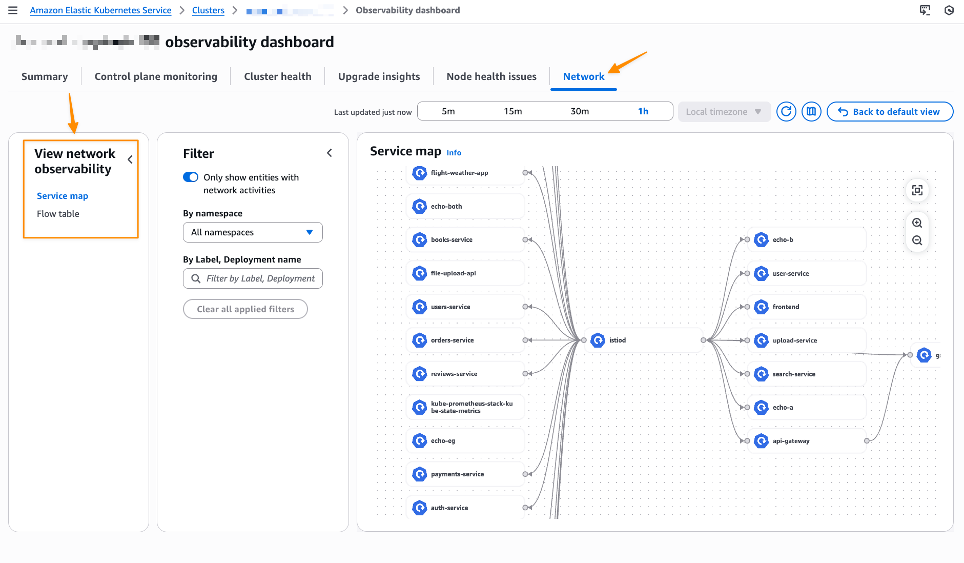
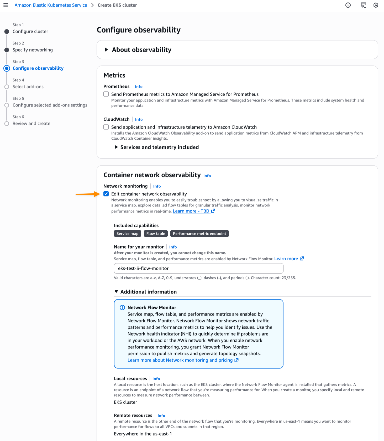
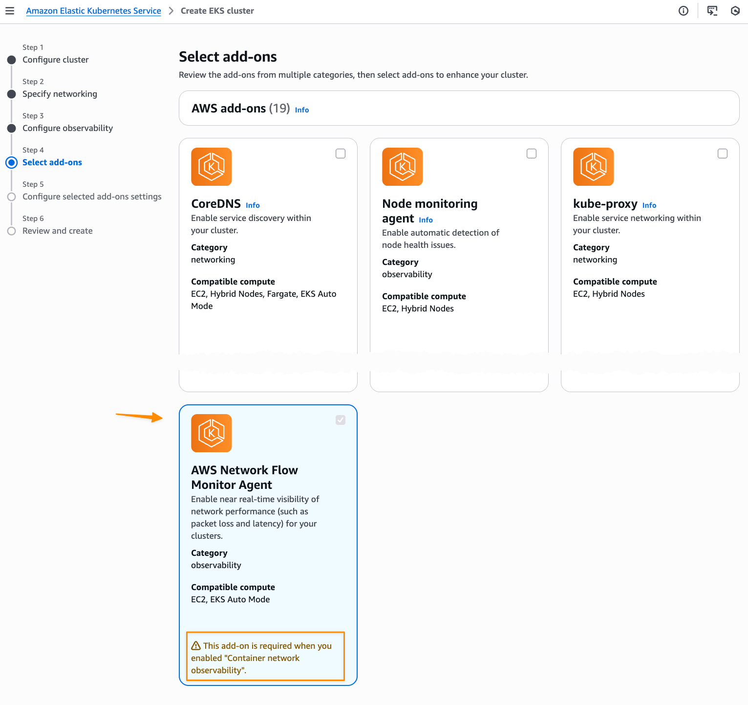
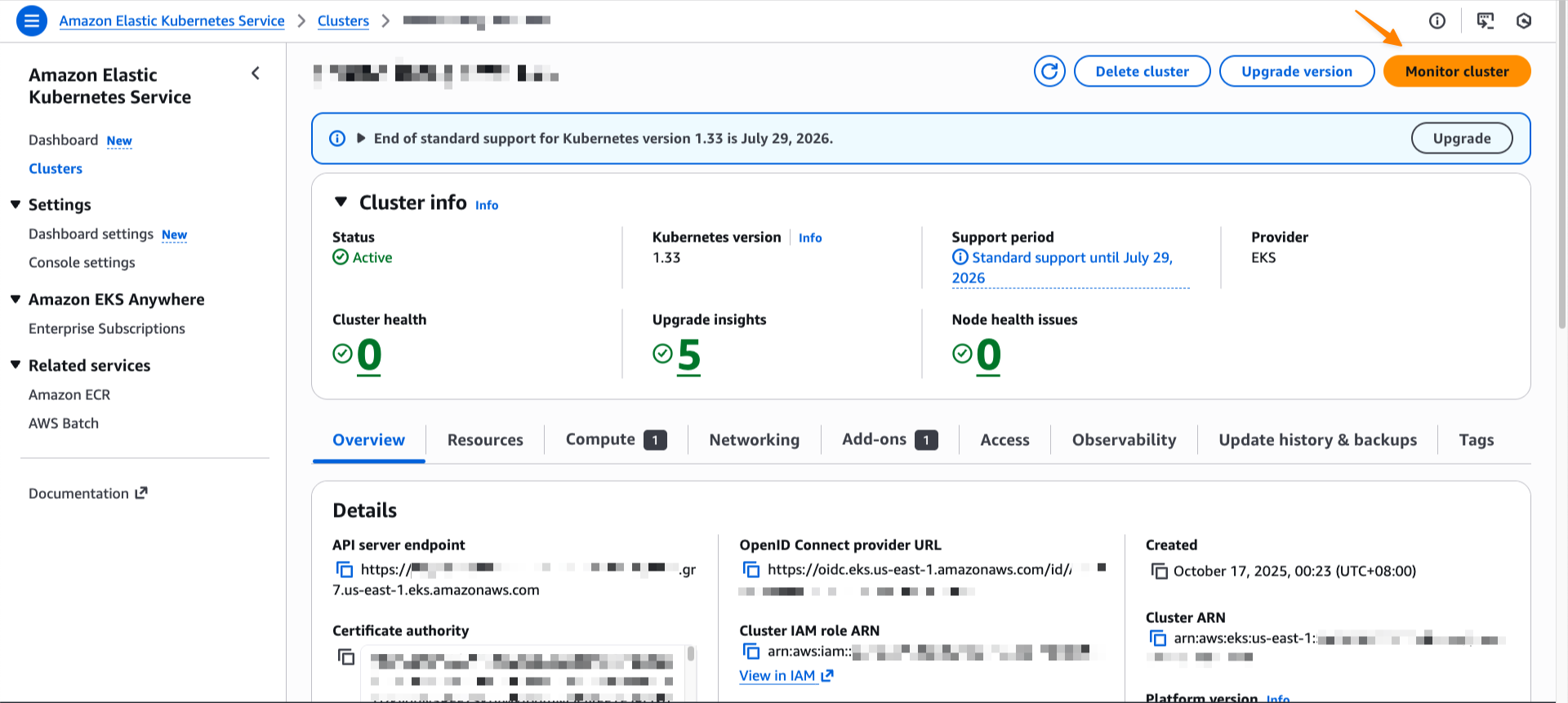
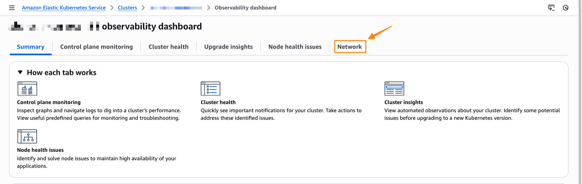
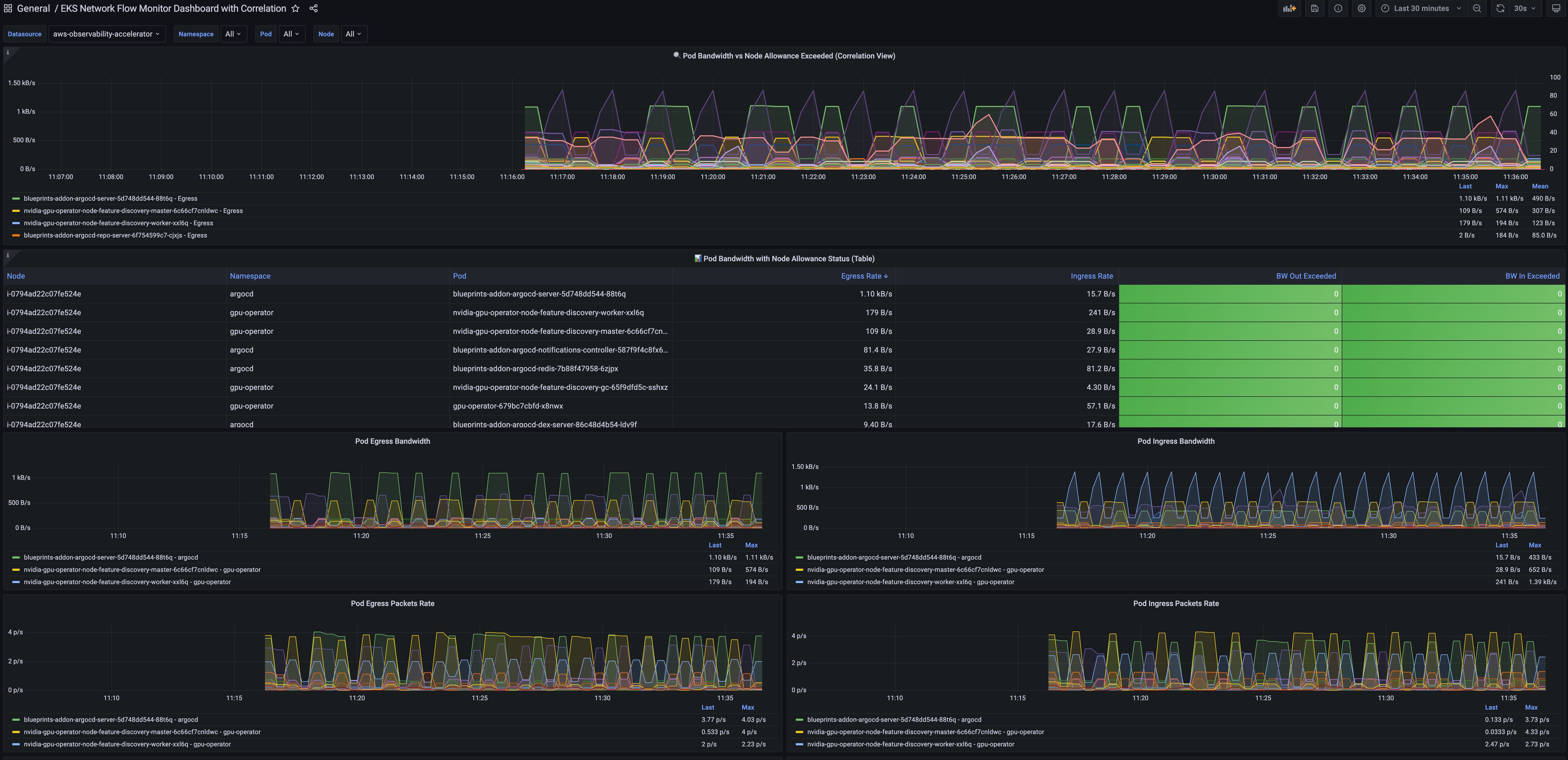
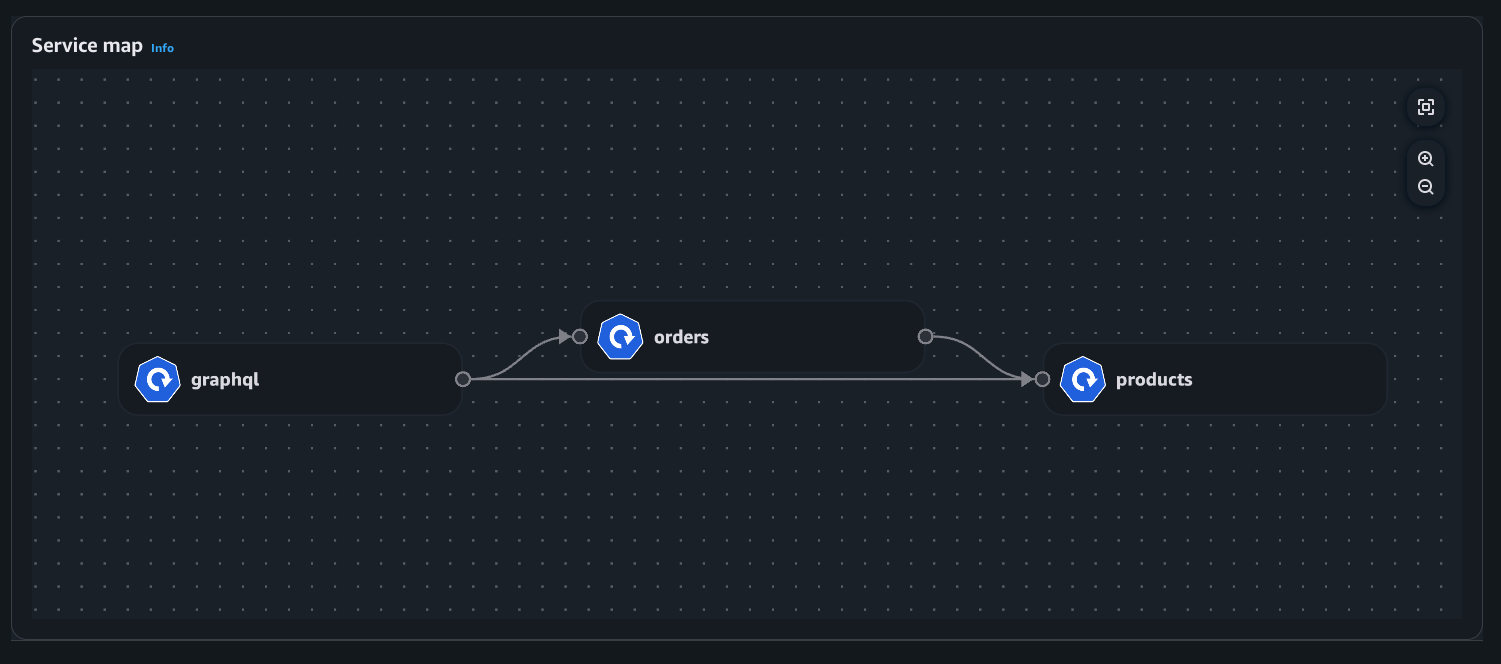
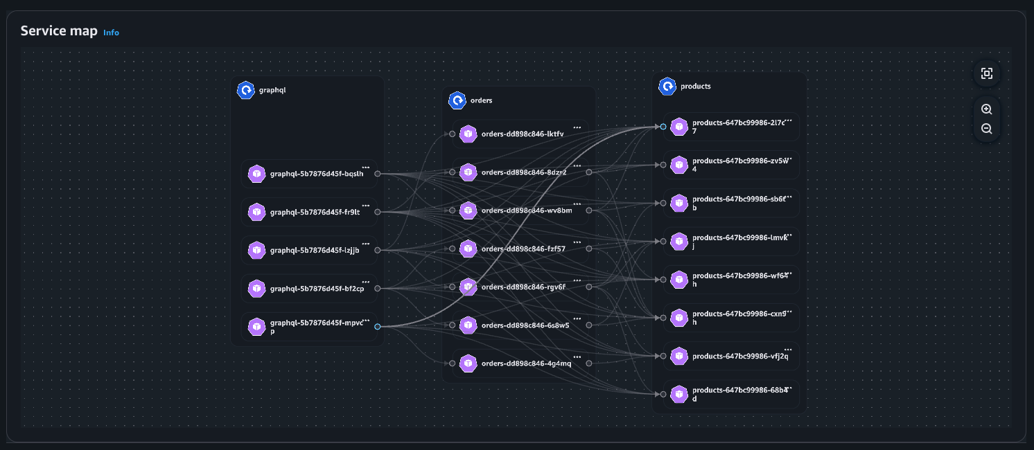
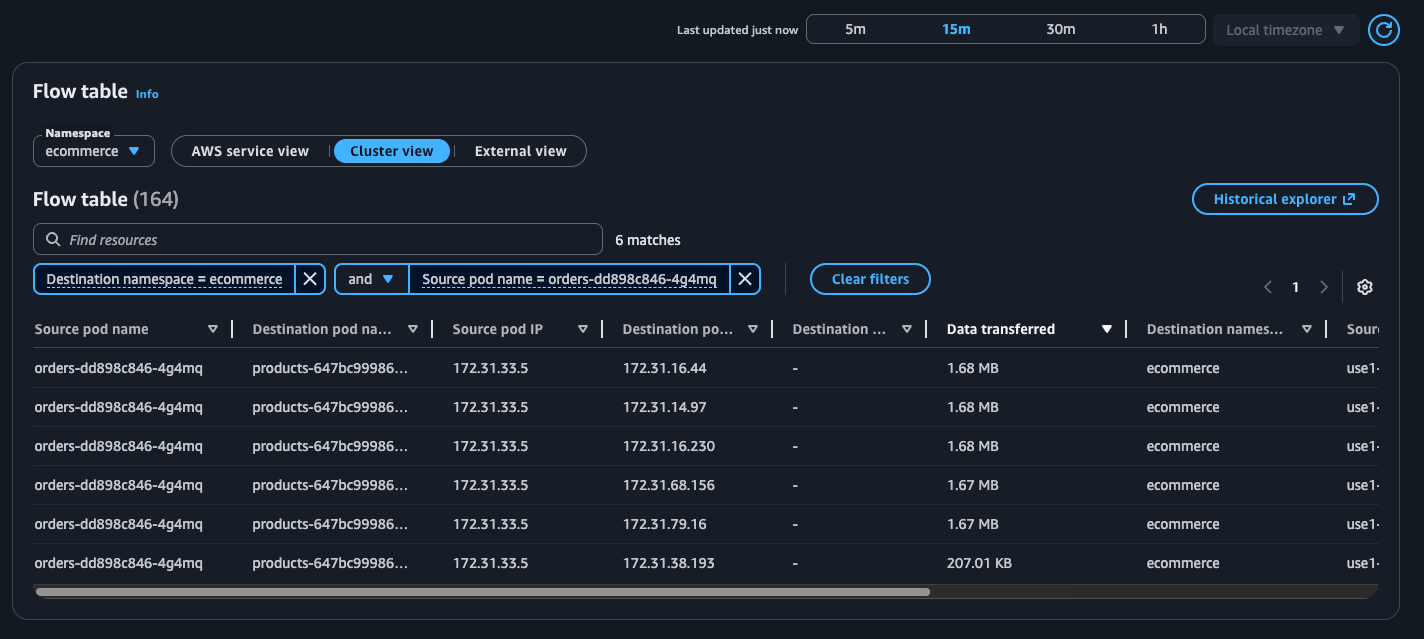
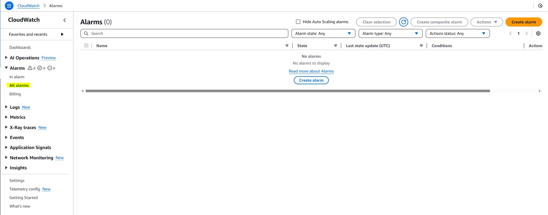
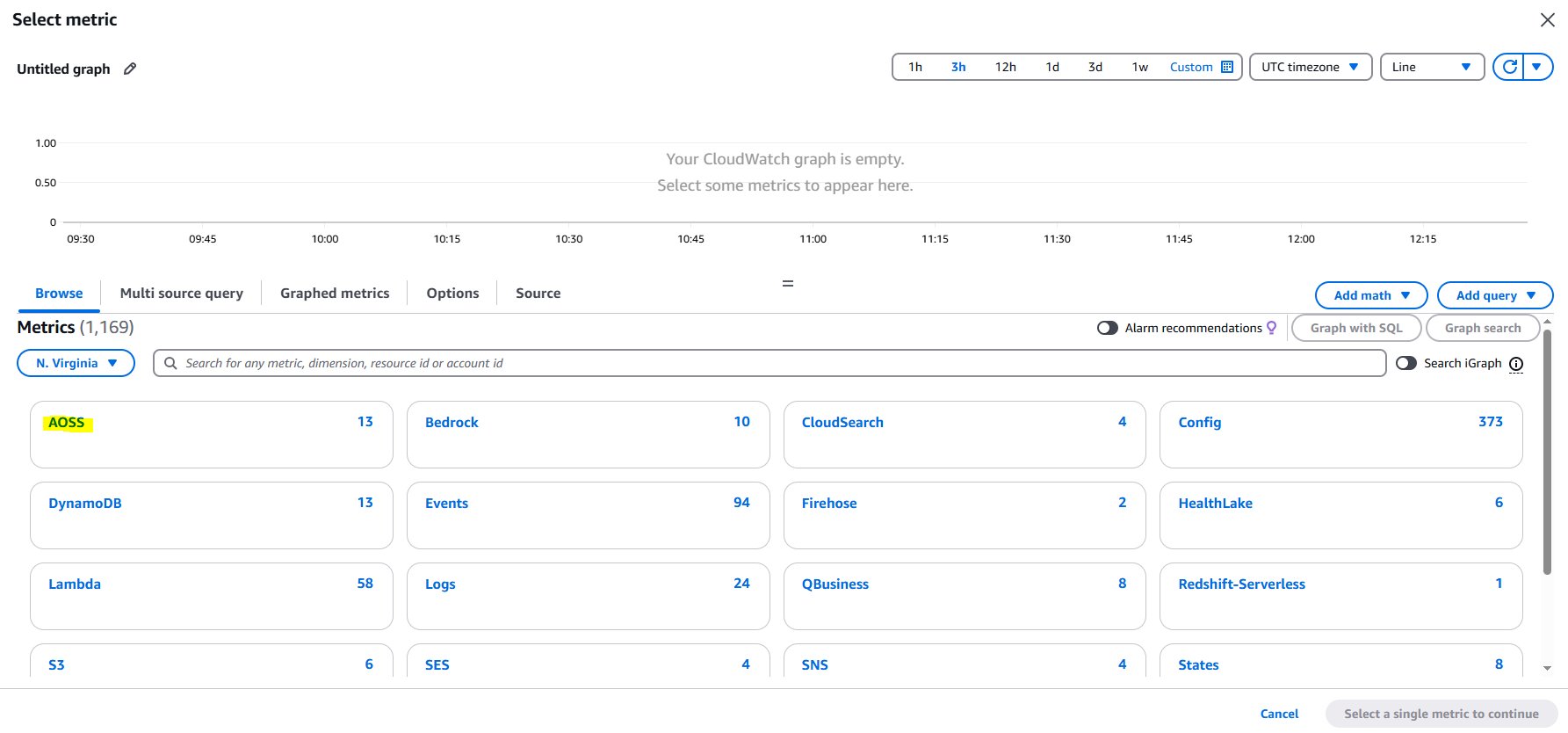
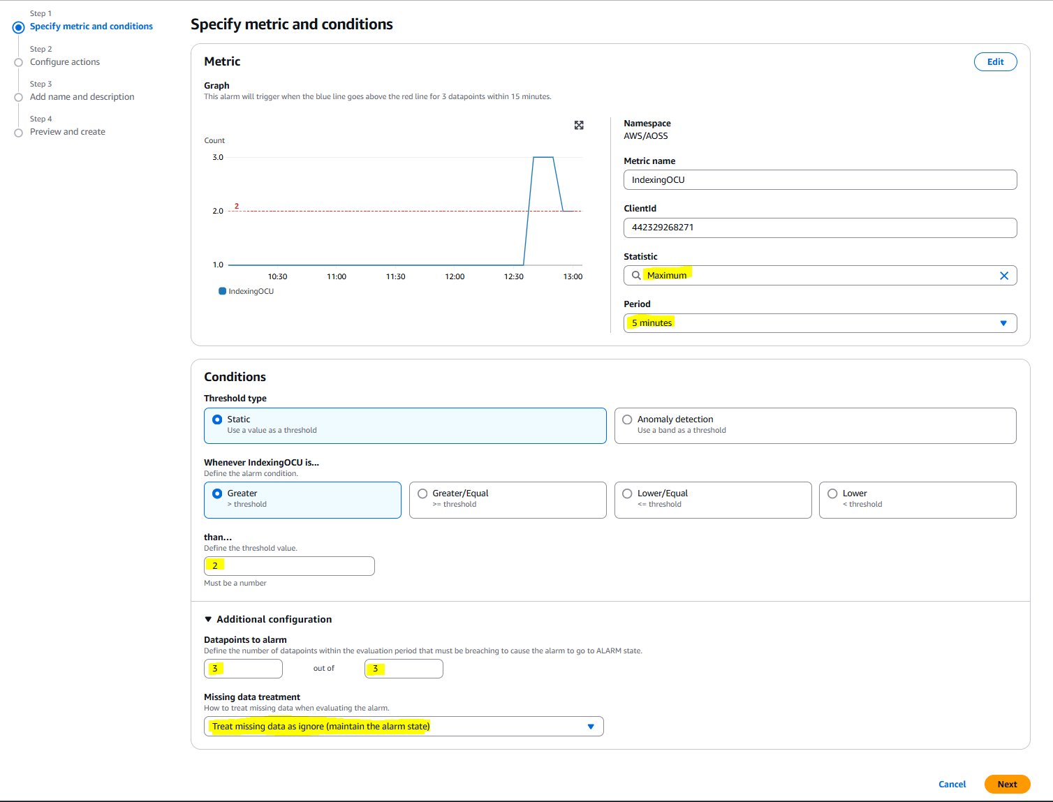
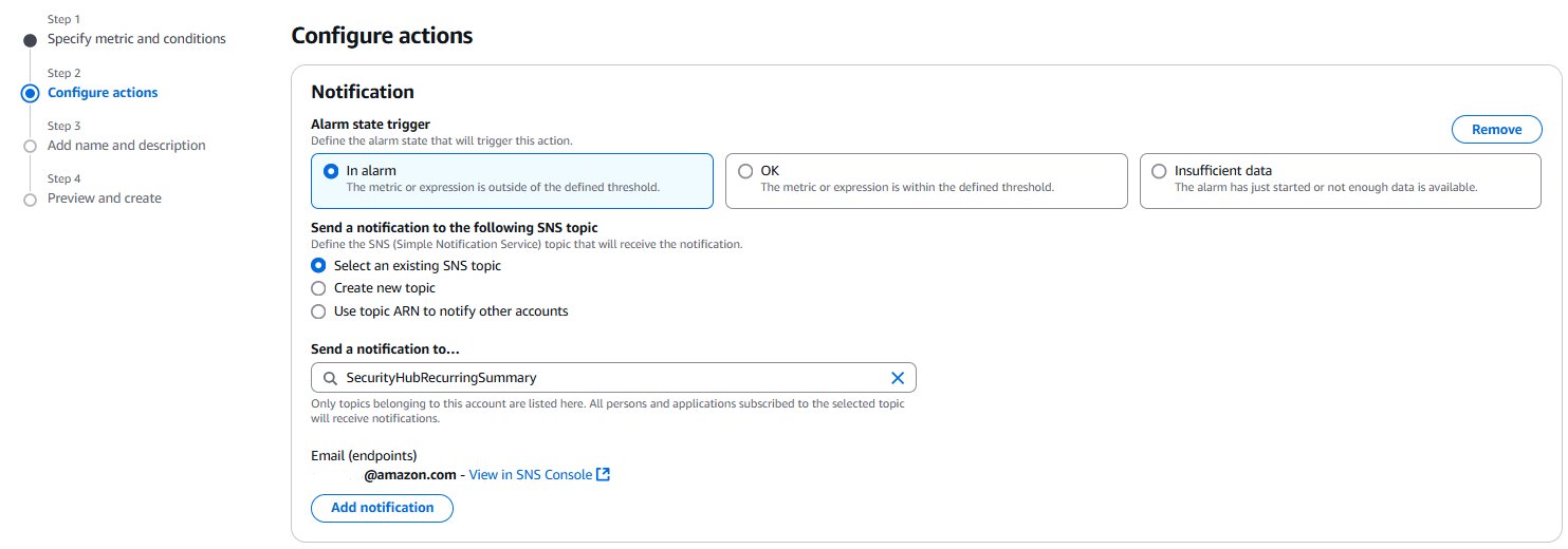
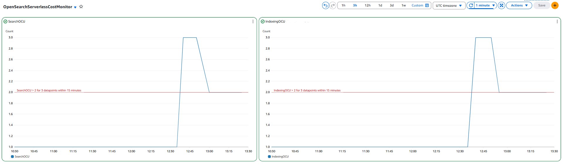
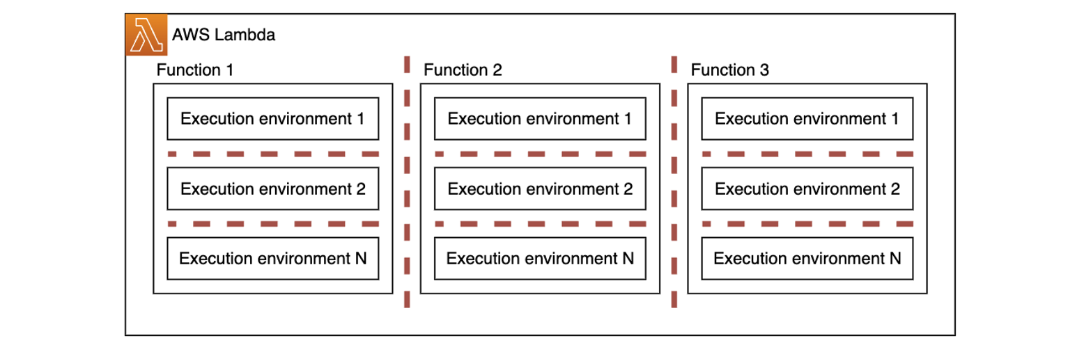
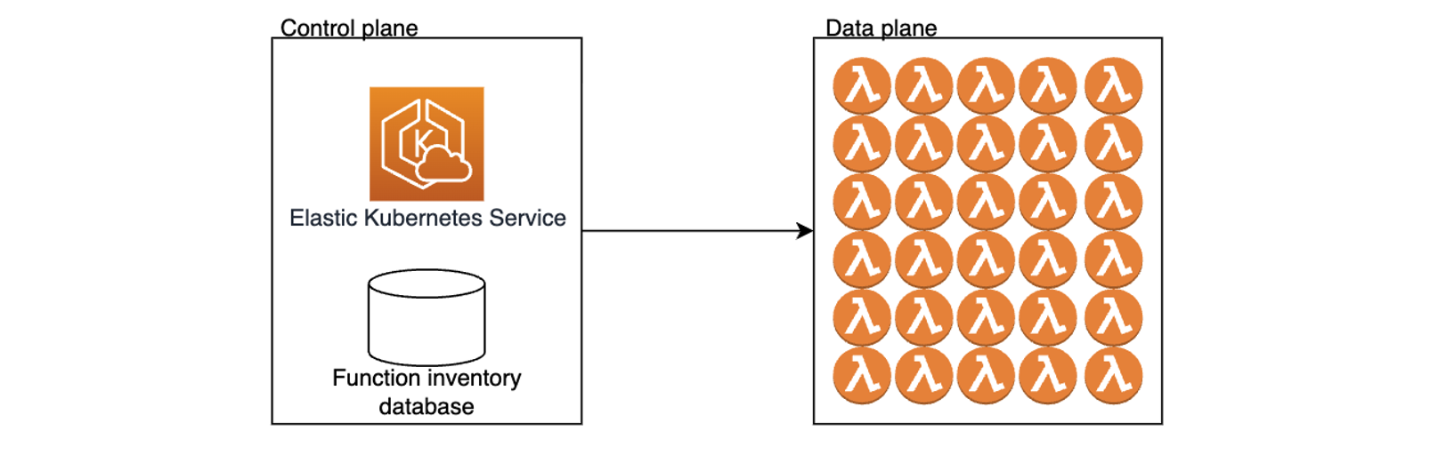
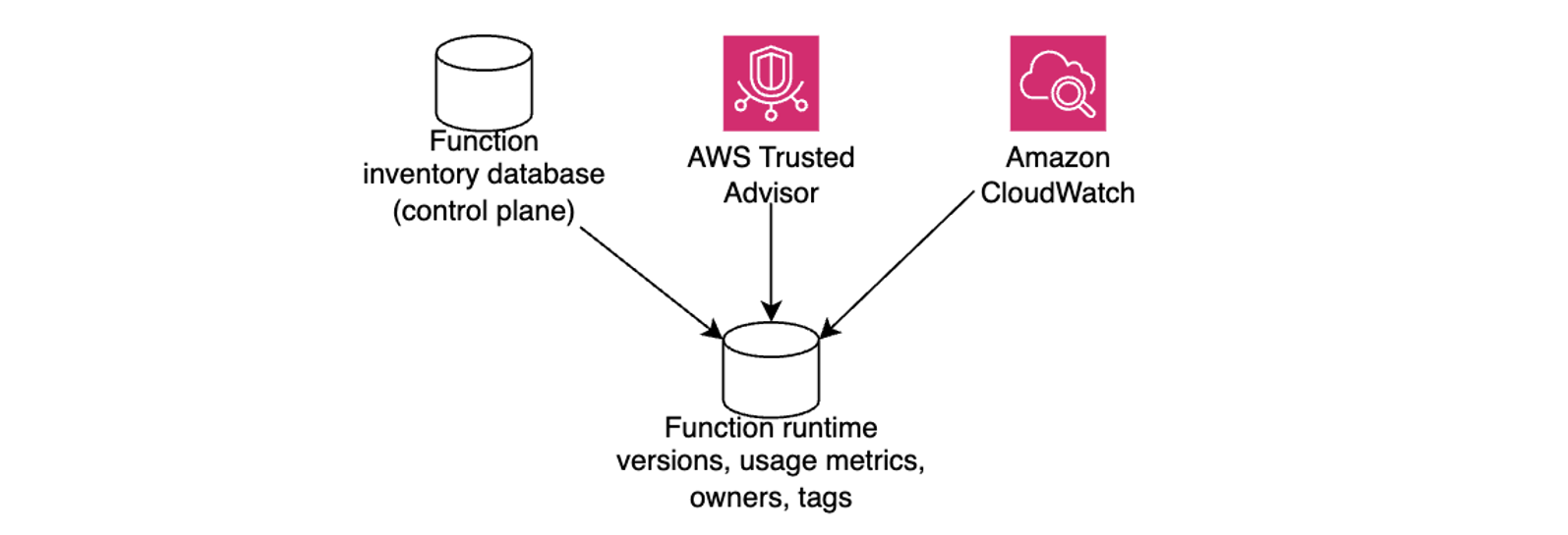
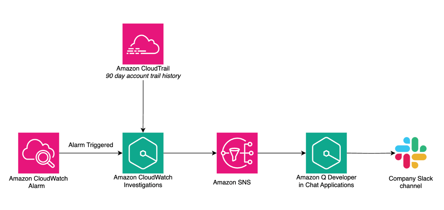
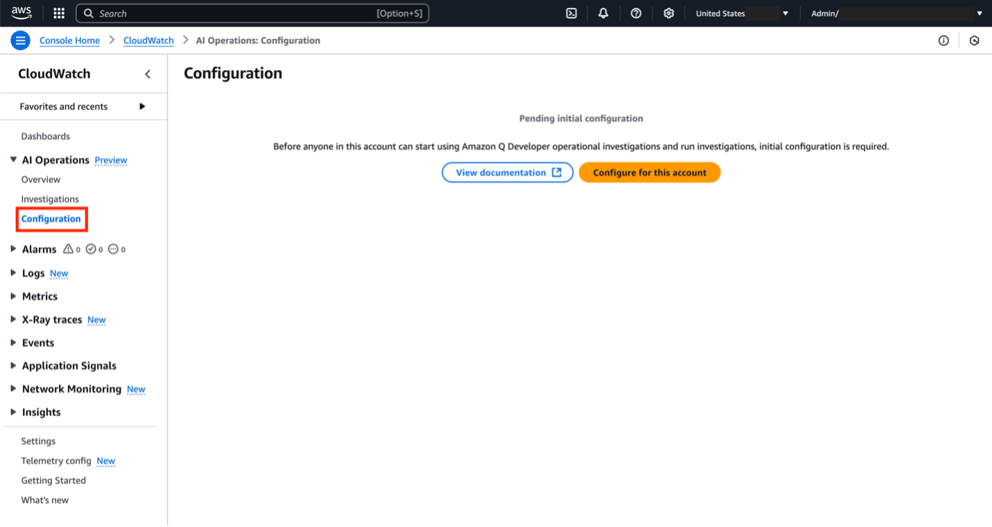
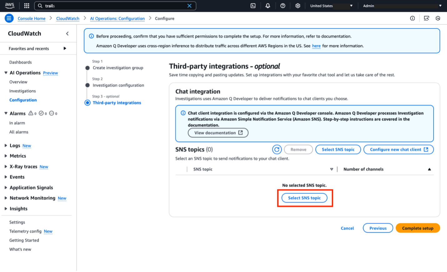
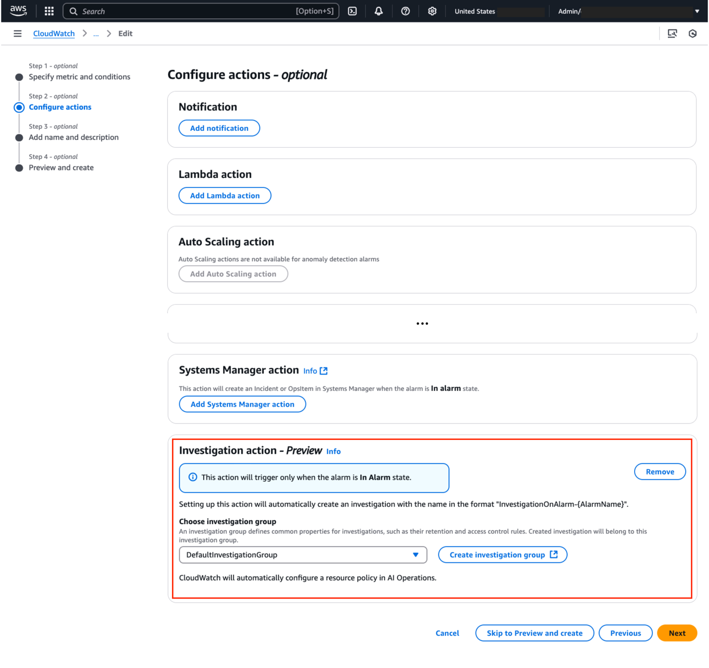
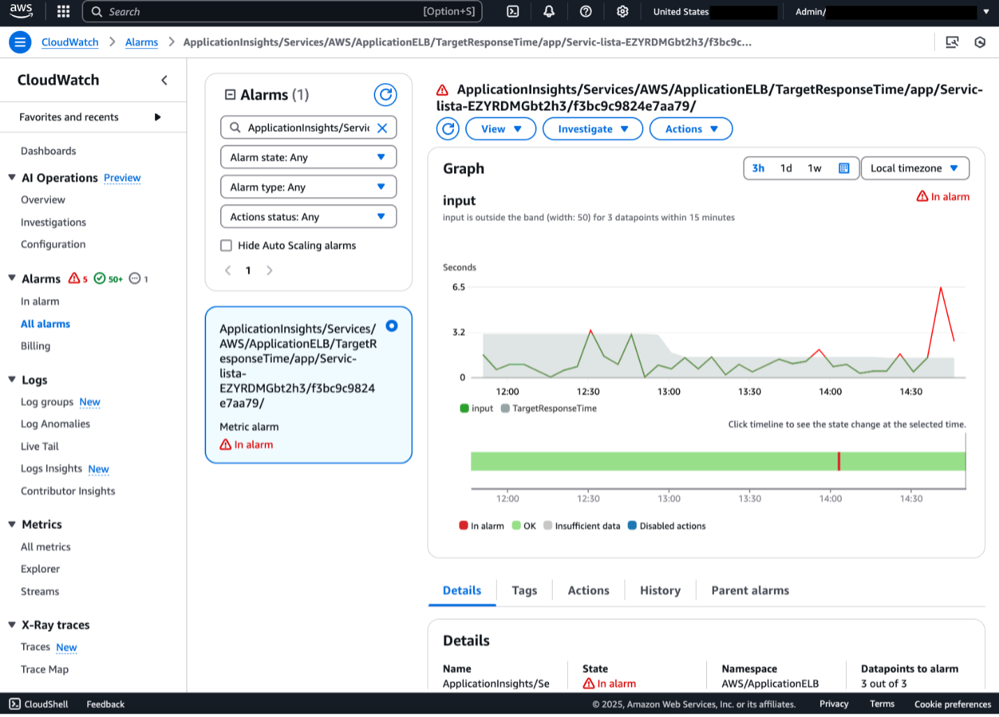
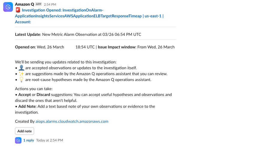
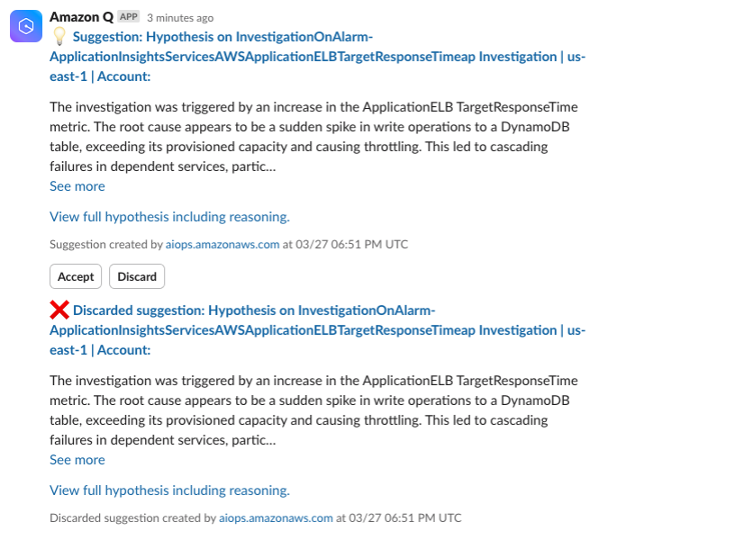
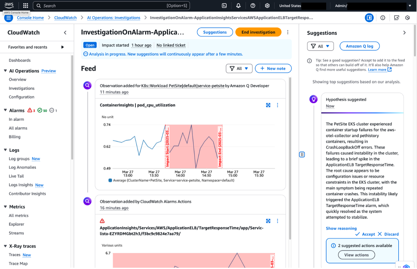


 Xiaoxue Xu is a Solutions Architect for AWS based in Toronto. She primarily works with financial services customers to help secure their workload and design scalable solutions on the AWS Cloud.
 Simran Singh is a Senior Solutions Architect at AWS. In this role, he assists our large enterprise customers in meeting their key business objectives using AWS. His areas of expertise include artificial intelligence and machine learning, security, and improving the experience of developers building on AWS.


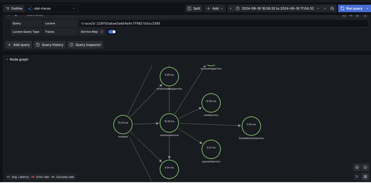
 Balaji Mohan is a Senior Delivery Consultant specializing in application and data modernization to the cloud. His business-first approach provides seamless transitions, aligning technology with organizational goals. Using cloud-centered architectures, he delivers scalable, agile, and cost-effective solutions, driving innovation and growth.
 Senthil Ramasamy is a Senior Database Consultant at Amazon Web Services. He works with AWS customers to provide guidance and technical assistance on database services, helping them with database migrations to the AWS Cloud and improving the value of their solutions when using AWS.
 Muthu Pitchaimani is a Search Specialist with Amazon OpenSearch Service. He builds large-scale search applications and solutions. Muthu is interested in the topics of networking and security, and is based out of Austin, Texas.
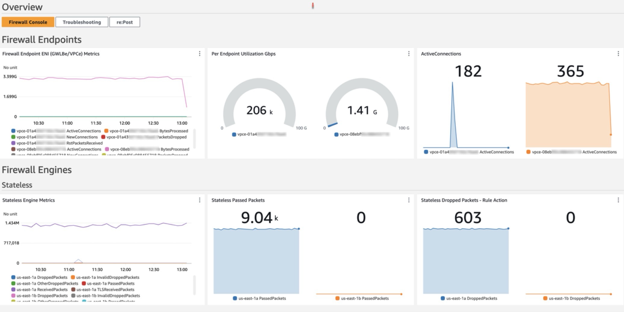
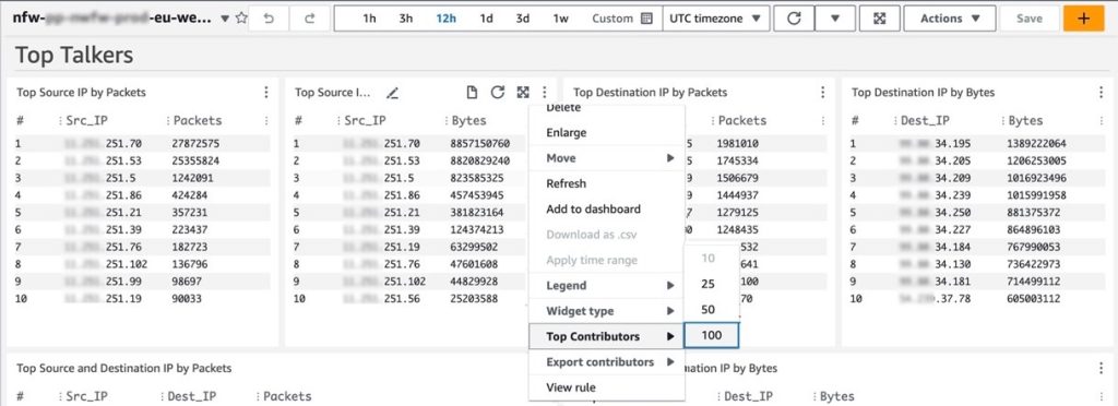
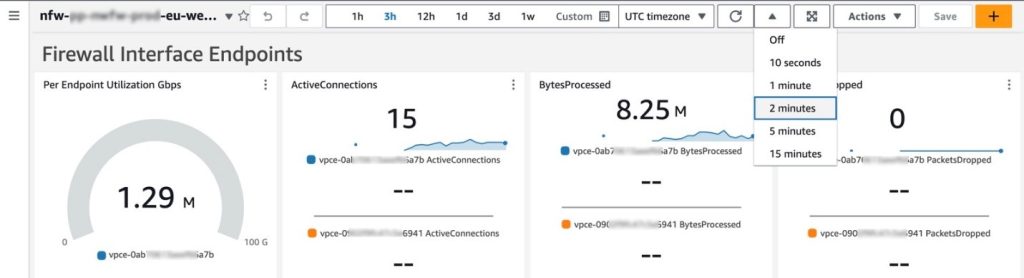
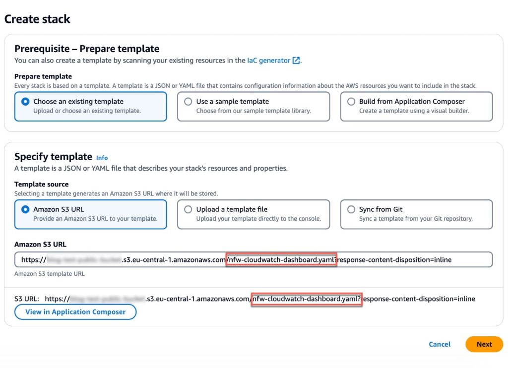


 Sumalatha Bachu is Senior Director, Technology at FINRA. She manages Big Data Operations which includes managing petabyte-scale data and complex workloads processing in cloud. Additionally, she is an expert in developing Enterprise Application Monitoring and Observability Solutions, Operational Data Analytics, & Machine Learning Model Governance work flows. Outside of work, she enjoys doing yoga, practicing singing, and teaching in her free time.
 PremKiran Bejjam is Lead Engineer Consultant at FINRA, specializing in developing resilient and scalable systems. With a keen focus on designing monitoring solutions to enhance infrastructure reliability, he is dedicated to optimizing system performance. Beyond work, he enjoys quality family time and continually seeks out new learning opportunities.
 Akhil Chalamalasetty is Director, Market Regulation Technology at FINRA. He is a Big Data subject matter expert specializing in building cutting edge solutions at scale along with optimizing workloads, data, and its processing capabilities. Akhil enjoys sim racing and Formula 1 in his free time.
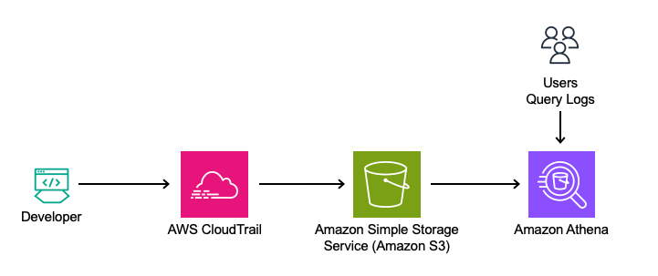
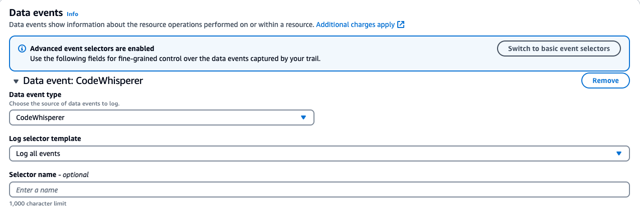


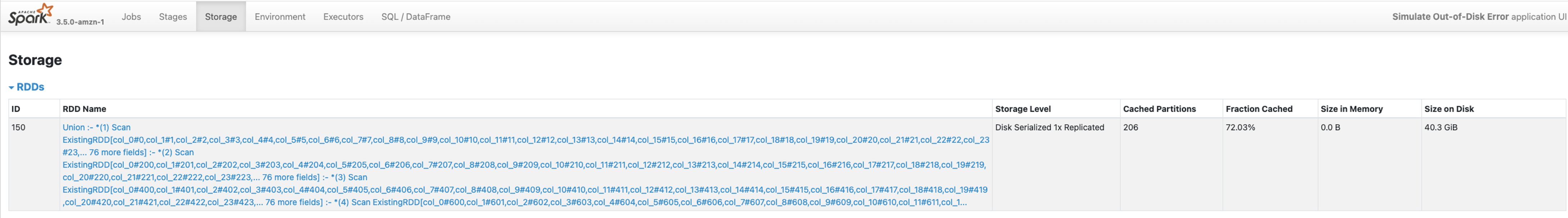
 Kashif Khan is a Sr. Analytics Specialist Solutions Architect at AWS, specializing in big data services like Amazon EMR, AWS Lake Formation, AWS Glue, Amazon Athena, and Amazon DataZone. With over a decade of experience in the big data domain, he possesses extensive expertise in architecting scalable and robust solutions. His role involves providing architectural guidance and collaborating closely with customers to design tailored solutions using AWS analytics services to unlock the full potential of their data.
 Veena Vasudevan is a Principal Partner Solutions Architect and Data & AI specialist at AWS. She helps customers and partners build highly optimized, scalable, and secure solutions; modernize their architectures; and migrate their big data, analytics, and AI/ML workloads to AWS.


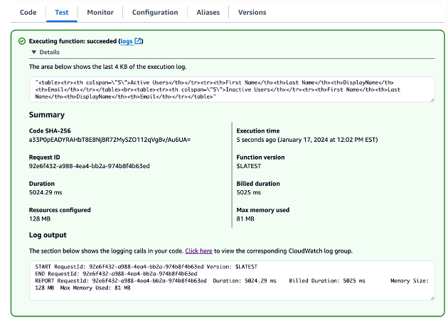


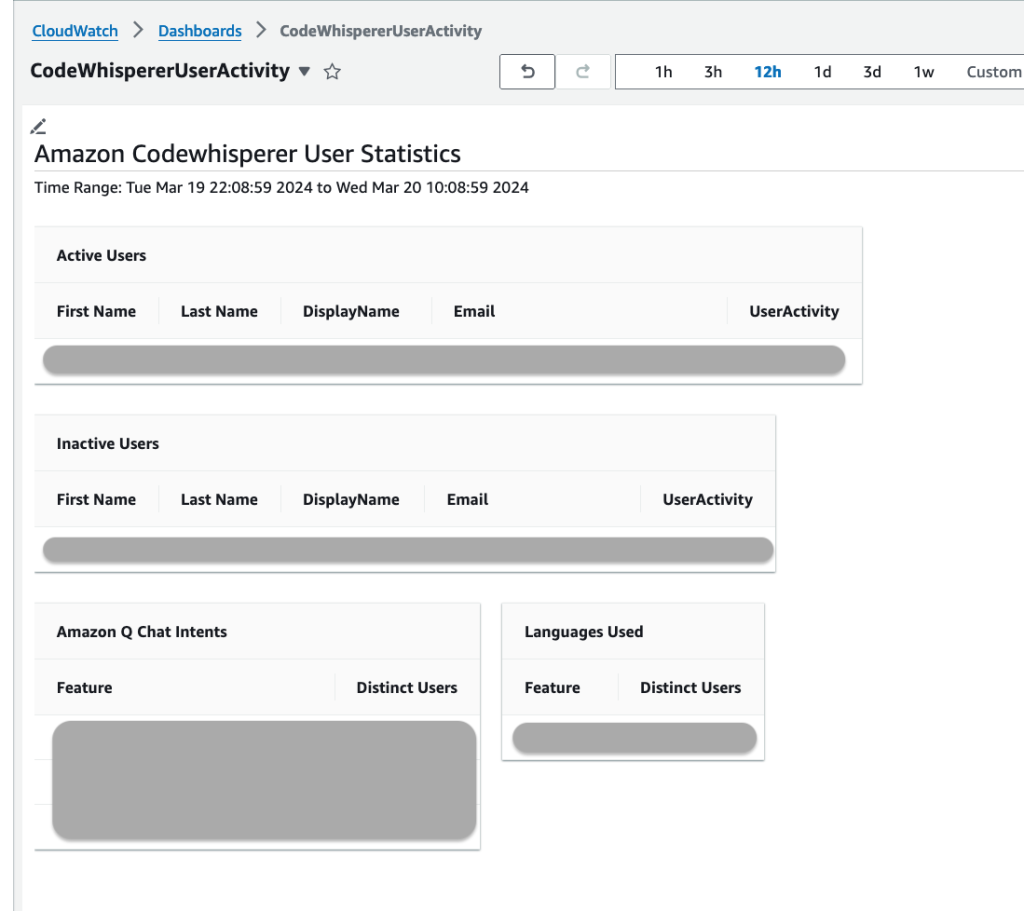


 Satesh Sonti is a Sr. Analytics Specialist Solutions Architect based out of Atlanta, specialized in building enterprise data platforms, data warehousing, and analytics solutions. He has over 17 years of experience in building data assets and leading complex data platform programs for banking and insurance clients across the globe.
 Harshida Patel is a Specialist Principal Solutions Architect, Analytics with AWS.
 Raghu Kuppala is an Analytics Specialist Solutions Architect experienced working in the databases, data warehousing, and analytics space. Outside of work, he enjoys trying different cuisines and spending time with his family and friends.
 Ashish Agrawal is a Sr. Technical Product Manager with Amazon Redshift, building cloud-based data warehouses and analytics cloud services. Ashish has over 24 years of experience in IT. Ashish has expertise in data warehouses, data lakes, and platform as a service. Ashish has been a speaker at worldwide technical conferences.


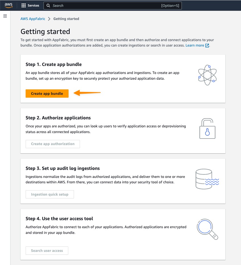
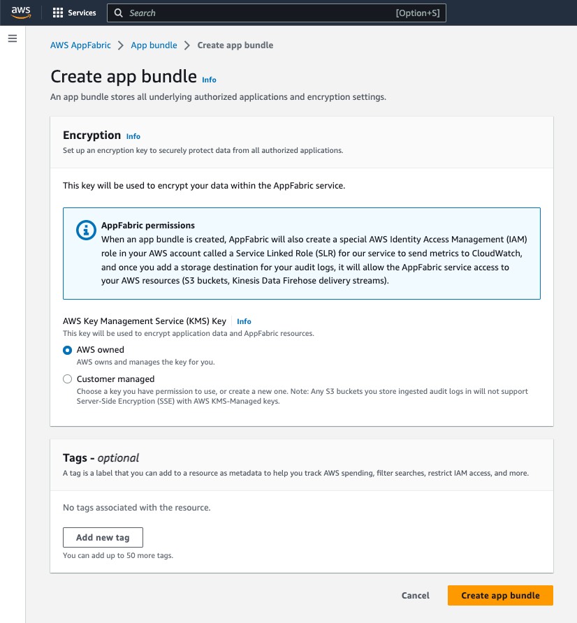

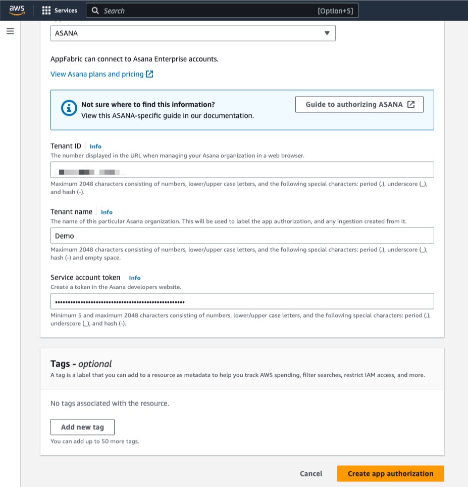
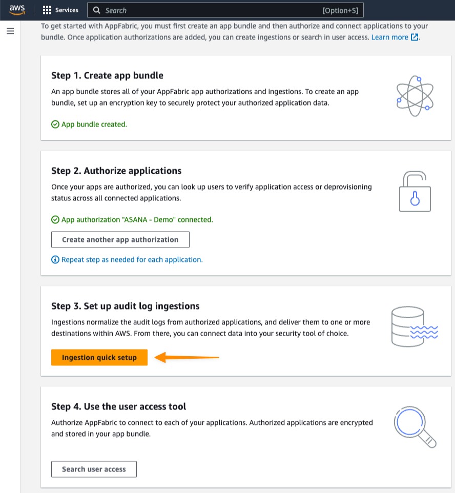
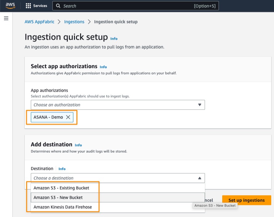
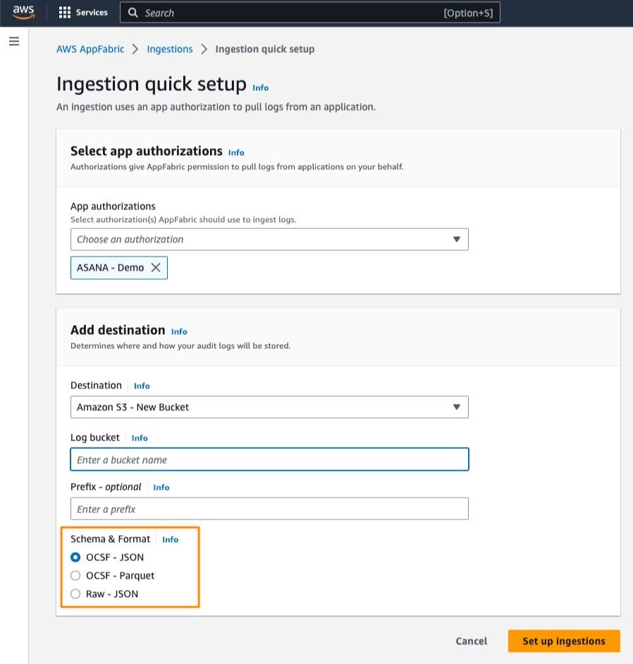


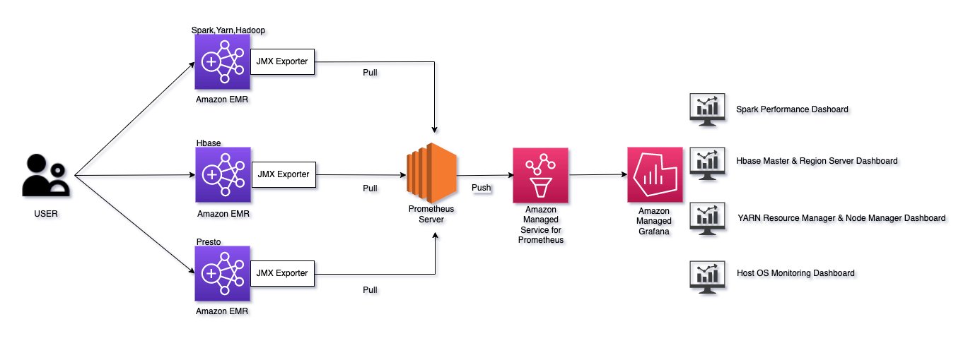


 Anubhav Awasthi is a Sr. Big Data Specialist Solutions Architect at AWS. He works with customers to provide architectural guidance for running analytics solutions on Amazon EMR, Amazon Athena, AWS Glue, and AWS Lake Formation.