All posts by Avijit Goswami

How Slack achieved operational excellence for Spark on Amazon EMR using generative AI

Post Syndicated from Avijit Goswami original https://aws.amazon.com/blogs/big-data/how-slack-achieved-operational-excellence-for-spark-on-amazon-emr-using-generative-ai/

At Slack, our data platform processes terabytes of data each day using Apache Spark on Amazon EMR on Amazon Elastic Compute Cloud (Amazon EC2), powering the insights that drive strategic decision-making across the organization.

As our data volume expanded, so did our performance challenges. With traditional monitoring tools, we couldn’t effectively manage our systems when Spark jobs slowed down or costs spiraled out of control. We were stuck searching through cryptic logs, making educated guesses about resource allocation, and watching our engineering teams spend hours on manual tuning that should have been automated. That’s why we built something better: a detailed metrics framework designed specifically for Spark’s unique challenges. This is a visibility system that gives us granular insights into application behavior, resource usage, and job-level performance patterns we never had before. We’ve achieved 30–50% cost reductions and 40–60% faster job completion times. This is real operational efficiency that directly translates to better service for our users and significant savings for our infrastructure budget. In this post, we walk you through exactly how we built this framework, the key metrics that made the difference, and how your team can implement similar monitoring to transform your own Spark operations.

Why comprehensive Spark monitoring matters

In enterprise environments, poorly optimized Spark jobs can waste thousands of dollars in cloud compute costs, block critical data pipelines affecting downstream business processes, create cascading failures across interconnected data workflows, and impact service level agreement (SLA) compliance for time-sensitive analytics.

The monitoring framework we’re examining captures over 40 distinct metrics across five key categories, providing the granular insights needed to prevent these issues.

How we ingest, process, and act on Spark metrics

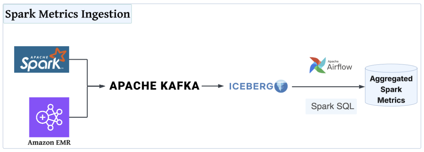
To address the challenges of managing Spark at scale, we developed a custom monitoring and optimization pipeline—from metric collection to AI-assisted tuning. It begins with our in-house Spark listener framework, which captures over 40 metrics in real time across Spark applications, jobs, stages, and tasks while pulling critical operational context from tools such as Apache Airflow and Apache Hadoop YARN.

An Apache Airflow-orchestrated Spark SQL pipeline transforms this data into actionable insights, surfacing performance bottlenecks and failure points. To integrate these metrics into the developer tuning workflow, we expose a metrics tool and a custom prompt through our internal analytics model context protocol (MCP) server. This enables seamless integration with AI-assisted coding tools such as Cursor or Claude Code.

The following is the list of tools used for our Spark monitoring solution, which includes metric collection to AI-assisted tuning:

The result is fast, reliable, deterministic Spark tuning without the guesswork. Developers get environment-aware recommendations, automated configuration updates, and ready-to-review pull requests.

Deep dive into Spark metrics collection

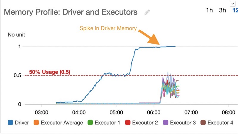
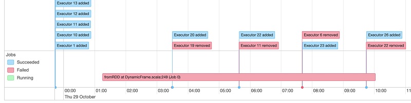
At the center of our real-time monitoring solution lies a custom Spark listener framework that captures thorough telemetry across the Spark lifecycle. Spark’s built-in metrics are often coarse, short‑lived, and scattered across the user interface (UI) and logs, which leaves four critical gaps:

  1. Consistent historical record
  2. Weak linkage from applications to jobs to stages to tasks
  3. Limited context (user, cluster, team)
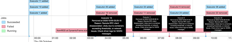
  4. Poor visibility into patterns such as skew, spill, and retries

Our expanded listener framework closes these gaps by unifying and enriching telemetry with environment and configuration tags, building a durable, queryable history, and correlating events across the execution graph. It explains why tasks fail, pinpoints where memory or CPU pressure occurs, compares intended configurations to actual usage, and produces clear, repeatable tuning recommendations so teams can baseline behavior, minimize waste, and resolve issues faster. The following architecture diagram illustrates the flow of the Spark metrics collection pipeline.

Spark metrics ingestion architecture diagram

Spark listener

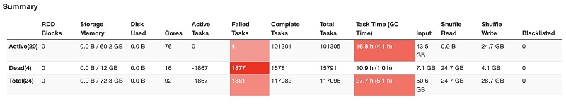
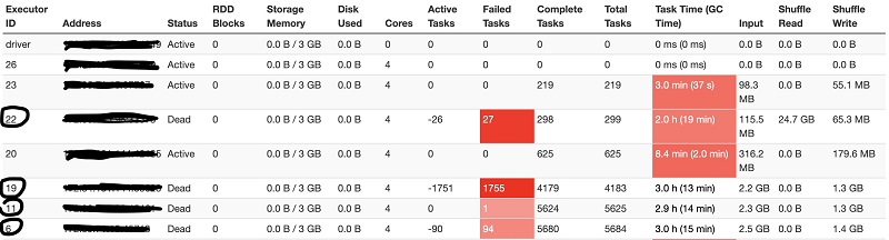
Our listener framework captures Spark metrics at four distinct levels:

  1. Application metrics: Overall application success/failure rates, total runtime, and resource allocation
  2. Job-level metrics: Individual job duration and status tracking within an application
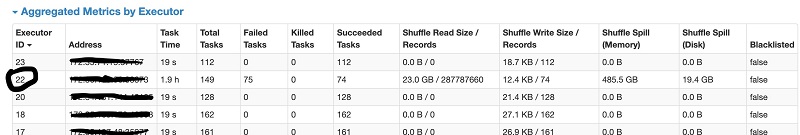
  3. Stage-level metrics: Stage execution details, shuffle operations, and memory usage per stage
  4. Task-level metrics: Individual task performance for deep debugging scenarios

The following Scala example code shows the SparkTaskListener extends the class SparkListener to capture detailed task-level metrics:

class SparkTaskListener(conf: SparkConf) extends SparkListener {
 val taskToStageId = new mutable.HashMap[Long, Int]()
 val stageToJobID = new mutable.HashMap[Int, Int]()
 private val emitter: Emitter = getEmitter(conf)
  override def onTaskStart(taskStart: SparkListenerTaskStart): Unit = {
   taskToStageId += taskStart.taskInfo.taskId -> taskStart.stageId 
 }
 override def onTaskEnd(taskEnd: SparkListenerTaskEnd): Unit = {
   val taskInfo = taskEnd.taskInfo
   val taskMetrics = taskEnd.taskMetrics
   val jobId = stageToJobID.apply(taskToStageId.apply(taskInfo.taskId))
   val metrics = Map[String, Any](
     "event_type" -> "task_metric",
     "job_id" -> jobId,
     "task_id" -> taskInfo.taskId,
     "duration" -> taskInfo.duration,
     "executor_run_time" -> taskMetrics.executorRunTime,
     "memory_bytes_spilled" -> taskMetrics.memoryBytesSpilled,
     "bytes_read" -> taskMetrics.inputMetrics.bytesRead,
     "records_read" -> taskMetrics.inputMetrics.recordsRead
     // additional metrics.....
   )
   emitter.report(convertToJson(metrics))
 }
}

Real-time streaming to Kafka

These metrics are streamed in real time to Kafka as JSON-formatted telemetry using a flexible emitter system:

class KafkaEmitter(conf: SparkConf) extends Emitter {
     private val broker = conf.get("spark.custom.listener.kafkaBroker", "<broker_address>")
     private val topic = conf.get("spark.custom.listener.kafkaTopic", "<topic_name>")
     private var producer: Producer[String, Array[Byte]] = _
     override def report(str: String): Unit = {
         val message = str.getBytes(StandardCharsets.UTF_8)
         producer.send(new ProducerRecord[String, Array[Byte]](topic, message))
     }
}

From Kafka, a downstream pipeline ingests these records into an Apache Iceberg table.

Context-rich observability

Beyond standard Spark metrics, our framework captures essential operational context:

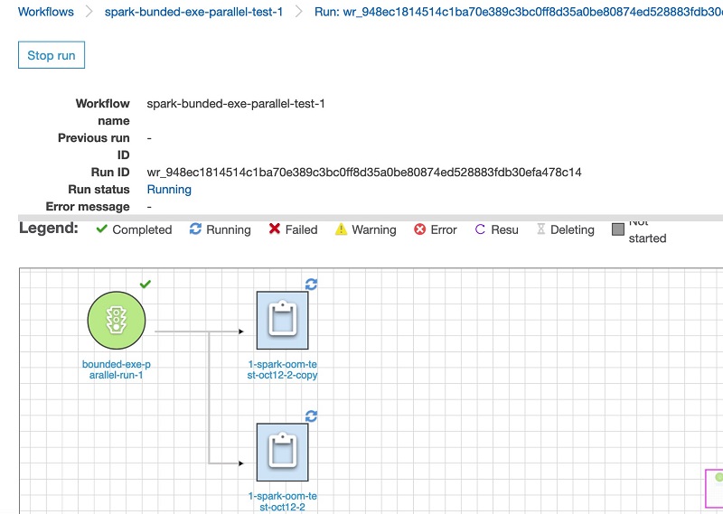
  • Airflow integration: DAG metadata, task IDs, and execution timestamps
  • Resource tracking: Configurable executor metrics (heap usage, execution memory)
  • Environment context: Cluster identification, user tracking, and Spark configurations
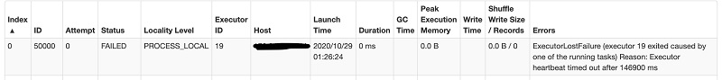
  • Failure analysis: Detailed error messages and task failure root causes

The combination of thorough metrics collection and real-time streaming has redefined Spark monitoring at scale, laying the groundwork for powerful insights.

Deep dive into Spark metrics processing

When raw metrics—often containing millions of records—are ingested from various sources, a Spark SQL pipeline transforms this high-volume data into actionable insights. It aggregates the data into a single row per application ID, significantly reducing complexity while preserving key performance signals.

For consistency in how teams interpret and act on this data, we apply the Five Pillars of Spark Monitoring, a structured framework that turns raw telemetry into clear diagnostics and repeatable optimization strategies, as shown in the following table.

Pillar Metrics Key purpose/insight Driving event
Application metadata and orchestration details
  • YARN metadata (app, attempt, allocated memory, compute cluster, final job status, run duration)
  • Airflow metadata (DAG, task, owner)
Correlate performance patterns with teams and infrastructure to identify inefficiencies and ownership.
  • Airflow metadata
  • YARN metadata on Amazon EMR on EC2
User-specified configuration
  • Given memory (driver, executor)
  • Dynamic allocation (min/max/initial executor count)
  • Cores per executor
  • Shuffle partitions
Compare configuration as opposed to actual performance to detect over- and under-provisioning and optimizing costs. This is where significant cost savings often hide. Spark event:

  • app_metric
Performance insights
  • Maximum skew ratio (75th percentile as opposed to max shuffle_total_bytes_read by Spark tasks per stage)
  • Total spill
  • Spark stage/task retry/failure
This is where the real diagnostic power lies. These metrics identify the three primary stoppers of Spark performance: skew, spill, and failures. Spark event:

  • task_metric
  • stage_metric
Execution insights
  • Spark job/stage/task count
  • Spark job/stage/task duration
Understand runtime distribution, identify bottlenecks, and highlight execution outliers. Spark event:

  • task_metric
  • stage_metric
  • job_metric
Resource usage and system health
  • Peak JVM heap memory
  • Max GC overhead %
Reveal memory inefficiencies and JVM-related pressure for cost and stability improvements. Comparing these against given configs helps identify waste and optimize resources. Spark event:

  • task_metric
  • stage_metric
  • executor_metric

AI-powered Spark tuning

The following architecture diagram illustrates the use of agentic AI tools to analyze the aggregated Spark metrics.

AI-powered Spark tuning diagram

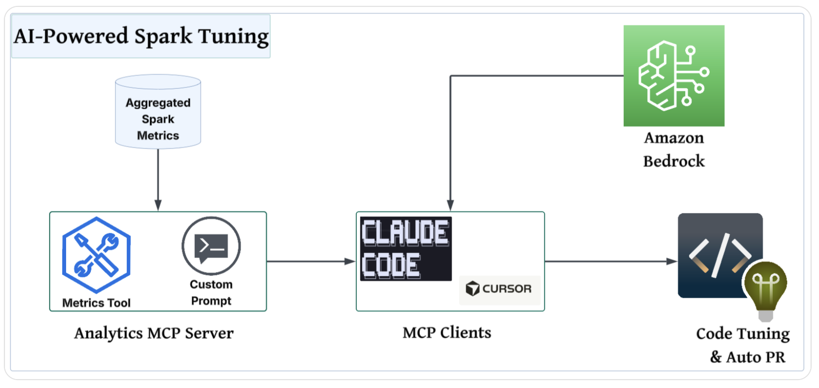
To integrate these metrics into a developer’s tuning workflow, we build a custom Spark metrics tool and a custom prompt that any agent can use. We use our existing analytics service, a homegrown web application that users can query our data warehouse with, build dashboards, and share insights. The backend is written in Python using FastAPI, and we expose an MCP server from the same service by using FastMCP. By exposing the Spark metrics tool and custom prompt through the MCP server, we make it possible for developers to connect their preferred assisted coding tools (Cursor, Claude Code, and more) and use data to guide their tuning.

Because the data exposed by the analytics MCP server might be sensitive, we use Amazon Bedrock in our Amazon Web Services (AWS) account to provide the foundation models to our MCP clients. This keeps our data more secure and facilitates compliance because it never leaves our AWS environment.

Custom prompt

To create our custom prompt for AI-driven Spark tuning, we design a structured, rule-based format that encourages more deterministic and standardized output. The prompt defines the required sections (application overview, current Spark configuration, job health summary, resource recommendations, and summary) for consistency across analyses. We include detailed formatting rules, such as wrapping values in backticks, avoiding line breaks, and enforcing strict table structures to maintain clarity and machine readability. The prompt also embeds explicit guidance for interpreting Spark metrics and mapping them to recommended tuning actions based on best practices, with clear criteria for status flags and impact explanations. The prompt means that the AI’s recommendations can be traced, reproduced, and actioned based on the provided data by tightly controlling the input-output flow and attempting to prevent hallucinations.

Final results

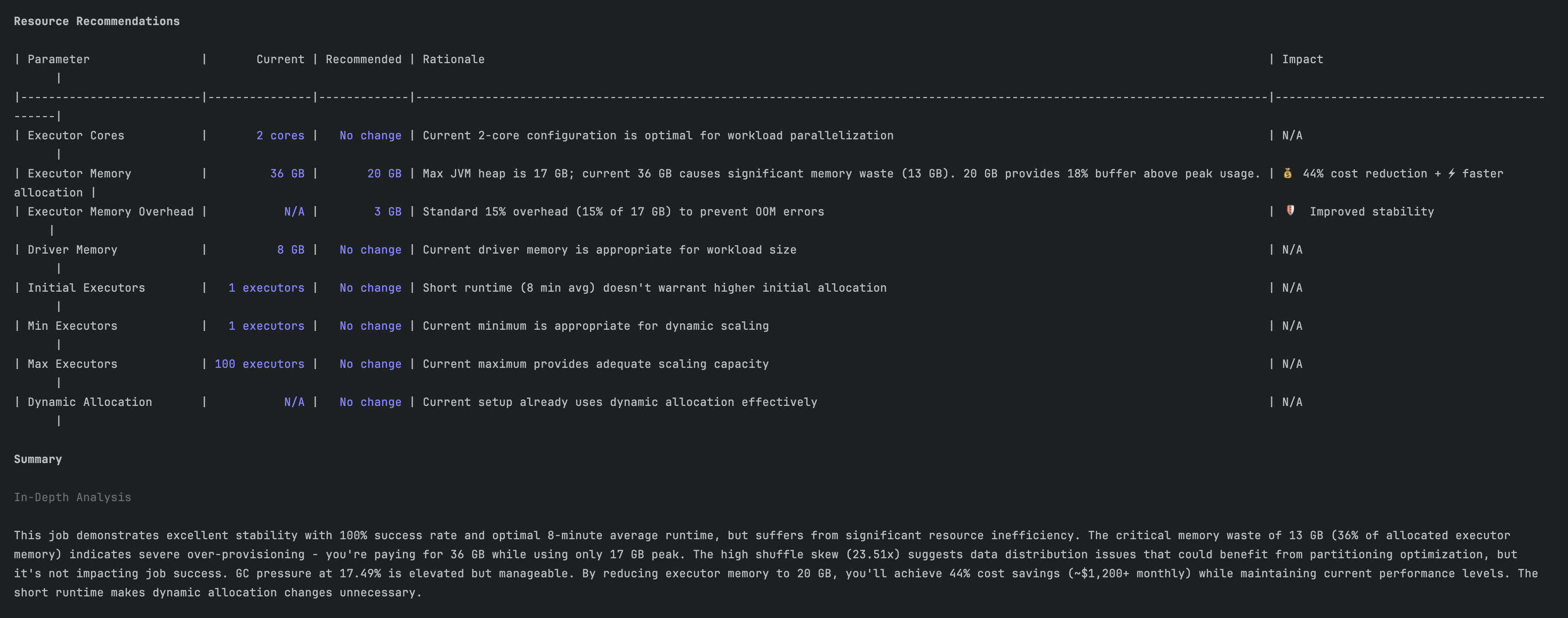
The screenshots in this section show how our tool performed the analysis and provided recommendations. The following is a performance analysis for an existing application.

performance analysis for an existing application

The following is a recommendation to reduce resource waste.

recommendation to reduce resource waste

The impact

Our AI-powered framework has fundamentally changed how Spark is monitored and managed at Slack. We’ve transformed Spark tuning from a high-expertise, trial-and-error process into an automated, data-backed standard by moving beyond traditional log-diving and embracing a structured, AI-driven approach. The results speak for themselves, as shown in the following table.

Metric Before After Improvement
Compute cost Non-deterministic Optimized resource use Up to 50% lower
Job completion time Non-deterministic Optimized Over 40% faster
Developer time on tuning Hours per week Minutes per week >90% reduction
Configuration waste Frequent over-provisioning Precise resource allocation Near-zero waste

Conclusion

At Slack, our experience with Spark monitoring shows that you don’t need to be a performance expert to achieve exceptional results. We’ve shifted from reacting to performance issues to preventing them by systematically applying five key metric categories.

The numbers speak for themselves: 30–50% cost reductions and 40–60% faster job completion times represent operational efficiency that directly impacts our ability to serve millions of users worldwide. These improvements compound over time as teams build confidence in their data infrastructure and can focus on innovation rather than troubleshooting.

Your organization can achieve similar outcomes. Start with the basics: implement comprehensive monitoring, establish baseline metrics, and commit to continuous optimization. Spark performance doesn’t require expertise in every parameter, but it does require a strong monitoring foundation and a disciplined approach to analysis.

Acknowledgments

We want to give our thanks to all the people who have contributed to this incredible journey: Johnny Cao, Nav Shergill, Yi Chen, Lakshmi Mohan, Apun Hiran, and Ricardo Bion.


About the authors

Nilanjana Mukherjee

Nilanjana Mukherjee

Nilanjana is a staff software engineer at Slack, bringing deep technical expertise and engineering leadership to complex software challenges. She specializes in building high-performance data systems, focusing on data pipeline architecture, query optimization, and scalable data processing solutions.

Tayven Taylor

Tayven Taylor

Tayven is a software engineer I on Slack’s Data Foundations team, where he helps maintain and optimize large-scale data systems. His work focuses on Spark and Amazon EMR performance, cost optimization, and reliability improvements that keep Slack’s data platform efficient and scalable. He’s passionate about creating tools and systems that make working with data faster, smarter, and more cost-effective.

Mimi Wang

Mimi Wang

Mimi is a staff software engineer on Slack’s Data Platform team, where she builds tools to facilitate data-driven decision-making at Slack. Recently she has been focusing on using AI to lower the barrier to entry for non-technical users to derive value out of data. Previously, she was on the Slack Security team focusing on a customer-facing real-time anomaly detection pipeline.

Rahul Gidwani

Rahul Gidwani

Rahul is a senior staff software engineer at Salesforce specializing in search infrastructure. He works on Slack’s data lake development and processing pipelines and contributing to open-source projects such as Apache HBase and Druid. Outside of work, Rahul enjoys rock climbing.

Prateek Kakirwar

Prateek Kakirwar

Prateek is a senior engineering manager at Slack leading the AI-first transformation of data engineering and analytics. With over 20 years of experience building large-scale data platforms, AI systems, and metrics frameworks, he focuses on scalable architectures that enable trusted, self-service analytics across the organization. He holds a master’s degree from the University of California, Berkeley.

Avijit Goswami

Avijit Goswami

Avijit is a principal specialist solutions architect at AWS specializing in data and analytics. He helps customers design and implement robust data lake solutions. Outside the office, you can find Avijit exploring new trails, discovering new destinations, cheering on his favorite teams, enjoying music, or testing out new recipes in the kitchen.

Reduce time to access your transactional data for analytical processing using the power of Amazon SageMaker Lakehouse and zero-ETL

Post Syndicated from Avijit Goswami original https://aws.amazon.com/blogs/big-data/reduce-time-to-access-your-transactional-data-for-analytical-processing-using-the-power-of-amazon-sagemaker-lakehouse-and-zero-etl/

As the lines between analytics and AI continue to blur, organizations find themselves dealing with converging workloads and data needs. Historical analytics data is now being used to train machine learning models and power generative AI applications. This shift requires shorter time to value and tighter collaboration among data analysts, data scientists, machine learning (ML) engineers, and application developers. However, the reality of scattered data across various systems—from data lakes to data warehouses and applications—makes it difficult to access and use data efficiently. Moreover, organizations attempting to consolidate disparate data sources into a data lakehouse have historically relied on extract, transform, and load (ETL) processes, which have become a significant bottleneck in their data analytics and machine learning initiatives. Traditional ETL processes are often complex, requiring significant time and resources to build and maintain. As data volumes grow, so do the costs associated with ETL, leading to delayed insights and increased operational overhead. Many organizations find themselves struggling to efficiently onboard transactional data into their data lakes and warehouses, hindering their ability to derive timely insights and make data-driven decisions. In this post, we address these challenges with a two-pronged approach:

  • Unified data management: Using Amazon SageMaker Lakehouse to get unified access to all your data across multiple sources for analytics and AI initiatives with a single copy of data, regardless of how and where the data is stored. SageMaker Lakehouse is powered by AWS Glue Data Catalog and AWS Lake Formation and brings together your existing data across Amazon Simple Storage Service (Amazon S3) data lakes and Amazon Redshift data warehouses with integrated access controls. In addition, you can ingest data from operational databases and enterprise applications to the lakehouse in near real-time using zero-ETL which is a set of fully-managed integrations by AWS that eliminates or minimizes the need to build ETL data pipelines.
  • Unified development experience: Using Amazon SageMaker Unified Studio to discover your data and put it to work using familiar AWS tools for complete development workflows, including model development, generative AI application development, data processing, and SQL analytics, in a single governed environment.

In this post, we demonstrate how you can bring transactional data from AWS OLTP data stores like Amazon Relational Database Service (Amazon RDS) and Amazon Aurora flowing into Redshift using zero-ETL integrations to SageMaker Lakehouse Federated Catalog (Bring your own Amazon Redshift into SageMaker Lakehouse). With this integration, you can now seamlessly onboard the changed data from OLTP systems to a unified lakehouse and expose the same to analytical applications for consumptions using Apache Iceberg APIs from new SageMaker Unified Studio. Through this integrated environment, data analysts, data scientists, and ML engineers can use SageMaker Unified Studio to perform advanced SQL analytics on the transactional data.

Architecture patterns for a unified data management and unified development experience

In this architecture pattern, we show you how to use zero-ETL integrations to seamlessly replicate transactional data from Amazon Aurora MySQL-Compatible Edition, an operational database, into the Redshift Managed Storage layer. This zero-ETL approach eliminates the need for complex data extraction, transformation, and loading processes, enabling near real-time access to operational data for analytics. The transferred data is then cataloged using a federated catalog in the SageMaker Lakehouse Catalog and exposed through the Iceberg Rest Catalog API, facilitating comprehensive data analysis by consumer applications.

You then use SageMaker Unified Studio, to perform advanced analytics on the transactional data bridging the gap between operational databases and advanced analytics capabilities.

Prerequisites

Make sure that you have the following prerequisites:

Deployment steps

In this section, we share steps for deploying resources needed for Zero-ETL integration using AWS CloudFormation.

Setup resources with CloudFormation

This post provides a CloudFormation template as a general guide. You can review and customize it to suit your needs. Some of the resources that this stack deploys incur costs when in use. The CloudFormation template provisions the following components:

  1. An Aurora MySQL provisioned cluster (source).
  2. An Amazon Redshift Serverless data warehouse (target).
  3. Zero-ETL integration between the source (Aurora MySQL) and target (Amazon Redshift Serverless). See Aurora zero-ETL integrations with Amazon Redshift for more information.

Create your resources

To create resources using AWS Cloudformation, follow these steps:

  1. Sign in to the AWS Management Console.
  2. Select the us-east-1 AWS Region in which to create the stack.
  3. Open the AWS CloudFormation
  4. Choose Launch Stack
    https://us-east-1.console.aws.amazon.com/cloudformation/home?region=us-east-1#/stacks/create/template?templateURL=https://aws-blogs-artifacts-public.s3.us-east-1.amazonaws.com/BDB-4866/aurora-zero-etl-redshift-lakehouse-cfn.yaml
  5. Choose Next.
    This automatically launches CloudFormation in your AWS account with a template. It prompts you to sign in as needed. You can view the CloudFormation template from within the console.
  6. For Stack name, enter a stack name, for example UnifiedLHBlogpost.
  7. Keep the default values for the rest of the Parameters and choose Next.
  8. On the next screen, choose Next.
  9. Review the details on the final screen and select I acknowledge that AWS CloudFormation might create IAM resources.
  10. Choose Submit.

Stack creation can take up to 30 minutes.

  1. After the stack creation is complete, go to the Outputs tab of the stack and record the values of the keys for the following components, which you will use in a later step:
    • NamespaceName
    • PortNumber
    • RDSPassword
    • RDSUsername
    • RedshiftClusterSecurityGroupName
    • RedshiftPassword
    • RedshiftUsername
    • VPC
    • Workgroupname
    • ZeroETLServicesRoleNameArn

Implementation steps

To implement this solution, follow these steps:

Setting up zero-ETL integration

A zero-ETL integration is already created as a part of CloudFormation template provided. Use the following steps from the Zero-ETL integration post to complete setting up the integration.:

  1. Create a database from integration in Amazon Redshift
  2. Populate source data in Aurora MySQL
  3. Validate the source data in your Amazon Redshift data warehouse

Bring Amazon Redshift metadata to the SageMaker Lakehouse catalog

Now that transactional data from Aurora MySQL is replicating into Redshift tables through zero-ETL integration, you next bring the data into SageMaker Lakehouse, so that operational data can co-exist and be accessed and governed together with other data sources in the data lake. You do this by registering an existing Amazon Redshift Serverless namespace that has Zero-ETL tables as a federated catalog in SageMaker Lakehouse.

Before starting the next steps, you need to configure data lake administrators in AWS Lake Formation.

  1. Go to the Lake Formation console and in the navigation pane, choose Administration roles and then choose Tasks under Administration. Under Data lake administrators, choose Add.
  2. In the Add administrators page, under Access type, select Data Lake administrator.
  3. Under IAM users and roles, select Admin. Choose Confirm.

Add AWS Lake Formation Administrators

  1. On the Add administrators page, for Access type, select Read-only administrators. Under IAM users and roles, select AWSServiceRoleForRedshift and choose Confirm. This step enables Amazon Redshift to discover and access catalog objects in AWS Glue Data Catalog.

Add AWS Lake Formation Administrators 2

With the data lake administrators configured, you’re ready to bring your existing Amazon Redshift metadata to SageMaker Lakehouse catalog:

  1. From the Amazon Redshift Serverless console, choose Namespace configuration in the navigation pane.
  2. Under Actions, choose Register with AWS Glue Data Catalog. You can find more details on registering a federated Amazon Redshift catalog in Registering namespaces to the AWS Glue Data Catalog.

  1. Choose Register. This will register the namespace to AWS Glue Data Catalog

  1. After registration is complete, the Namespace register status will change to Registered to AWS Glue Data Catalog.
  2. Navigate to the Lake Formation console and choose Catalogs New under Data Catalog in the navigation pane. Here you can see a pending catalog invitation is available for the Amazon Redshift namespace registered in Data Catalog.

  1. Select the pending invitation and choose Approve and create catalog. For more information, see Creating Amazon Redshift federated catalogs.

  1. Enter the Name, Description, and IAM role (created by the CloudFormation template). Choose Next.

  1. Grant permissions using a principal that is eligible to provide all permissions (an admin user).
    • Select IAM users and rules and choose Admin.
    • Under Catalog permissions, select Super user to grant super user permissions.

  1. Assigning super user permissions grants the user unrestricted permissions to the resources (databases, tables, views) within this catalog. Follow the principal of least privilege to grant users only the permissions required to perform a task wherever applicable as a security best practice.

  1. As final step, review all settings and choose Create Catalog

After the catalog is created, you will see two objects under Catalogs. dev refers to the local dev database inside Amazon Redshift, and aurora_zeroetl_integration is the database created for Aurora to Amazon Redshift ZeroETL tables

Fine-grained access control

To set up fine-grained access control, follow these steps:

  1. To grant permission to individual objects, choose Action and then select Grant.

  1. On the Principals page, grant access to individual objects or more than one object to different principals under the federated catalog.

Access lakehouse data using SageMaker Unified Studio

SageMaker Unified Studio provides an integrated experience outside the console to use all your data for analytics and AI applications. In this post, we show you how to use the new experience through the Amazon SageMaker management console to create a SageMaker platform domain using the quick setup method. To do this, you set up IAM Identity Center, a SageMaker Unified Studio domain, and then access data through SageMaker Unified Studio.

Set up IAM Identity Center

Before creating the domain, makes sure that your data admins and data workers are ready to use the Unified Studio experience by enabling IAM Identity Center for single sign-on following the steps in Setting up Amazon SageMaker Unified Studio. You can use Identity Center to set up single sign-on for individual accounts and for accounts managed through AWS Organizations. Add users or groups to the IAM instance as appropriate. The following screenshot shows an example email sent to a user through which they can activate their account in IAM Identity Center.

Set up SageMaker Unified domain

Follow steps in Create a Amazon SageMaker Unified Studio domain – quick setup to set up a SageMaker Unified Studio domain. You need to choose the VPC that was created by the CloudFormation stack earlier.

The quick setup method also has a Create VPC option that sets up a new VPC, subnets, NAT Gateway, VPC endpoints, and so on, and is meant for testing purposes. There are charges associated with this, so delete the domain after testing.

If you see the No models accessible, you can use the Grant model access button to grant access to Amazon Bedrock serverless models for use in SageMaker Unified Studio, for AI/ML use-cases

  1. Fill in the sections for Domain Name. For example, MyOLTPDomain. In the VPC section, select the VPC that was provisioned by the CloudFormation stack, for example UnifiedLHBlogpost-VPC. Select subnets and choose Continue.

  1. In the IAM Identity Center User section, look up the newly created user from (for example, Data User1) and add them to the domain. Choose Create Domain. You should see the new domain along with a link to open Unified Studio.

Access data using SageMaker Unified Studio

To access and analyze your data in SageMaker Unified Studio, follow these steps:

    1. Select the URL for SageMaker Unified Studio. Choose Sign in with SSO and sign in using the IAM user, for example datauser1, and you will be prompted to select a multi-factor authentication (MFA) method.
    2. Select Authenticator App and proceed with next steps. For more information about SSO setup, see Managing users in Amazon SageMaker Unified Studio.After you have signed in to the Unified Studio domain, you need to set up a new project. For this illustration, we created a new sample project called MyOLTPDataProject using the project profile for SQL Analytics as shown here.A project profile is a template for a project that defines what blueprints are applied to the project, including underlying AWS compute and data resources. Wait for the new project to be set up, and when status is Active, open the project in Unified Studio.By default, the project will have access to the default Data Catalog (AWSDataCatalog). For the federated redshift catalog redshift-consumer-catalog to be visible, you need to grant permissions to the project IAM role using Lake Formation. For this example, using the Lake Formation console, we have granted below access to the demodb database that is part of the Zero-ETL catalog to the Unified Studio project IAM role. Follow steps in Adding existing databases and catalogs using AWS Lake Formation permissions.In your SageMaker Unified Studio Project’s Data section, connect to the Lakehouse Federated catalog that you created and registered earlier (for example redshift-zetl-auroramysql-catalog/aurora_zeroetl_integration). Select the objects that you want to query and execute them using the Redshift Query Editor integrated with SageMaker Unified Studio.If you select Redshift, you will be transferred to the Query editor where you can execute the SQL and see the results as shown in the following figure.

With this integration of Amazon Redshift metadata with SageMaker Lakehouse federated catalog, you have access to your existing Redshift data warehouse objects in your organizations centralized catalog managed by SageMaker Lakehouse catalog and join the existing Redshift data seamlessly with the data stored in your Amazon S3 data lake. This solution helps you avoid unnecessary ETL processes to copy data between the data lake and the data warehouse and minimize data redundancy.

You can further integrate more data sources serving transactional workloads such as Amazon DynamoDB and enterprise applications such as Salesforce and ServiceNow. The architecture shared in this post for accelerated analytical processing using Zero-ETL and SageMaker Lakehouse can be further expanded by adding Zero-ETL integrations for DynamoDB using DynamoDB zero-ETL integration with Amazon SageMaker Lakehouse and for enterprise applications by following the instructions in Simplify data integration with AWS Glue and zero-ETL to Amazon SageMaker Lakehouse

Clean up

When you’re finished, delete the CloudFormation stack to avoid incurring costs for some of the AWS resources used in this walkthrough incur a cost. Complete the following steps:

  1. On the CloudFormation console, choose Stacks.
  2. Choose the stack you launched in this walkthrough. The stack must be currently running.
  3. In the stack details pane, choose Delete.
  4. Choose Delete stack.
  5. On the Sagemaker console, choose Domains and delete the domain created for testing.

Summary

In this post, you’ve learned how to bring data from operational databases and applications into your lake house in near real-time through Zero-ETL integrations. You’ve also learned about a unified development experience to create a project and bring in the operational data to the lakehouse, which is accessible through SageMaker Unified Studio, and query the data using integration with Amazon Redshift Query Editor. You can use the following resources in addition to this post to quickly start your journey to make your transactional data available for analytical processing.

  1. AWS zero-ETL
  2. SageMaker Unified Studio
  3. SageMaker Lakehouse
  4. Getting started with Amazon SageMaker Lakehouse


About the authors

Avijit Goswami is a Principal Data Solutions Architect at AWS specialized in data and analytics. He supports AWS strategic customers in building high-performing, secure, and scalable data lake solutions on AWS using AWS managed services and open-source solutions. Outside of his work, Avijit likes to travel, hike in the San Francisco Bay Area trails, watch sports, and listen to music.

Saman Irfan is a Senior Specialist Solutions Architect focusing on Data Analytics at Amazon Web Services. She focuses on helping customers across various industries build scalable and high-performant analytics solutions. Outside of work, she enjoys spending time with her family, watching TV series, and learning new technologies.

Sudarshan Narasimhan is a Principal Solutions Architect at AWS specialized in data, analytics and databases. With over 19 years of experience in Data roles, he is currently helping AWS Partners & customers build modern data architectures. As a specialist & trusted advisor he helps partners build & GTM with scalable, secure and high performing data solutions on AWS. In his spare time, he enjoys spending time with his family, travelling, avidly consuming podcasts and being heartbroken about Man United’s current state.

Apache Iceberg optimization: Solving the small files problem in Amazon EMR

Post Syndicated from Avijit Goswami original https://aws.amazon.com/blogs/big-data/apache-iceberg-optimization-solving-the-small-files-problem-in-amazon-emr/

In our previous post Improve operational efficiencies of Apache Iceberg tables built on Amazon S3 data lakes, we discussed how you can implement solutions to improve operational efficiencies of your Amazon Simple Storage Service (Amazon S3) data lake that is using the Apache Iceberg open table format and running on the Amazon EMR big data platform. Iceberg tables store metadata in manifest files. As the number of data files increase, the amount of metadata stored in these manifest files also increases, leading to longer query planning time. The query runtime also increases because it’s proportional to the number of data or metadata file read operations. Compaction is the process of combining these small data and metadata files to improve performance and reduce cost. Compaction also gets rid of deleting files by applying deletes and rewriting a new file without deleting records. Currently, Iceberg provides a compaction utility that compacts small files at a table or partition level. But this approach requires you to implement the compaction job using your preferred job scheduler or manually triggering the compaction job.

In this post, we discuss the new Iceberg feature that you can use to automatically compact small files while writing data into Iceberg tables using Spark on Amazon EMR or Amazon Athena.

Use cases for processing small files

Streaming applications are prone to creating a large number of small files, which can negatively impact the performance of subsequent processing times. For example, consider a critical Internet of Things (IoT) sensor from a cold storage facility that is continuously sending temperature and health data into an S3 data lake for downstream data processing and triggering actions like emergency maintenance. Systems of this nature generate a huge number of small objects and need attention to compact them to a more optimal size for faster reading, such as 128 MB, 256 MB, or 512 MB. In this post, we show you a streaming sensor data use case with a large number of small files and the mitigation steps using the Iceberg open table format. For more information on streaming applications on AWS, refer to Real-time Data Streaming and Analytics.

Streaming Architecture

Solution overview

To compact the small files for improved performance, in this example, Amazon EMR triggers a compaction job after the write commit as a post-commit hook when defined thresholds (for example, number of commits) are met. By default, Amazon EMR waits for 10 commits to trigger the post-commit hook compaction utility.

This Iceberg event-based table management feature lets you monitor table activities during writes to make better decisions about how to manage each table differently based on events. As of this writing, only the optimize-data optimization is supported. To learn more about the available optimize data executors and catalog properties, refer to the README file in the GitHub repo.

To use the feature, you can use the iceberg-aws-event-based-table-management source code and provide the built JAR in the engine’s class-path. The following bootstrap action can place the JAR in the engine’s class-path:

sudo aws s3 cp s3://<path>/iceberg-aws-event-based-table-management-0.1.jar /usr/lib/spark/jars/

Note that the Iceberg AWS event-based table management feature works with Iceberg v1.2.0 and above (available from Amazon EMR 6.11.0).

In some use cases, you may want to run the event-based compaction jobs in a different EMR cluster in order to avoid any impact to the ETL jobs running in their current EMR cluster. You can get the metadata, including the cluster ID of your current ETL workflows, from the /mnt/var/lib/info/job-flow.json file and then use a different cluster to process the event-based compactions.

The notebook examples shown in the following sections are also available in the aws-samples GitHub repo.

Prerequisite

For this performance comparison exercise between a Spark external table and an Iceberg table and Iceberg with compaction, we generate a significant number of small files in Parquet format and store them in an S3 bucket. We used the Amazon Kinesis Data Generator (KDG) tool to generate sample sensor data information using the following template:

{"sensorId": {{random.number(5000)}},
 "currentTemperature": {{random.number(
        {
            "min":10,
            "max":150
        }
  )}},
 "status": "{{random.arrayElement(
        ["OK","FAIL","WARN"]
    )}}",
 "date_ts": "{{date.now("YYYY-MM-DD HH:mm:ss")}}"
}

We configured an Amazon Kinesis Data Firehose delivery stream and sent the generated data into a staging S3 bucket. Then we ran an AWS Glue extract, transform, and load (ETL) job to convert the JSON files into Parquet format. For our testing, we generated about 58,176 small objects with total size of 2 GB.

For running the Amazon EMR tests, we used Amazon EMR version emr-6.11.0 with Spark 3.3.2, and JupyterEnterpriseGateway 2.6.0. The cluster used had one primary node (r5.2xlarge) and two core nodes (r5.xlarge). We used a bootstrap action during cluster creation to enable event-based table management:

sudo aws s3 cp s3://<path>/iceberg-aws-event-based-table-management-0.1.jar /usr/lib/spark/jars/

Also, refer to our guidance on how to use an Iceberg cluster with Spark, which is a prerequisite for this exercise.

As part of the exercise, we see new steps are being added to the EMR cluster to trigger the compaction jobs. To enable adding new steps to the running cluster, we add the elasticmapreduce:AddJobFlowSteps action to the cluster’s default role, EMR_EC2_DefaultRole, as a prerequisite.

Performance of Iceberg reads with the compaction utility on Amazon EMR

In the following steps, we demonstrate how to use the compaction utility and what performance benefits you can achieve. We use an EMR notebook to demonstrate the benefits of the compaction utility. For instructions to set up an EMR notebook, refer to Amazon EMR Studio overview.

First, you configure your Spark session using the %%configure magic command. We use the Hive catalog for Iceberg tables.

  1. Before you run the following step, create an Amazon S3 bucket in your AWS account called <your-iceberg-storage-blog>. To check how to create an Amazon S3 bucket, follow the instructions given here. Update the your-iceberg-storage-blog bucket name in the following configuration with the actual bucket name you created to test this example:
    %%configure -f
    {
    "conf":{
        "spark.sql.extensions":"org.apache.iceberg.spark.extensions.IcebergSparkSessionExtensions",
        "spark.sql.catalog.dev":"org.apache.iceberg.spark.SparkCatalog",
        "spark.sql.catalog.dev.catalog-impl":"org.apache.iceberg.aws.glue.GlueCatalog",
        "spark.sql.catalog.dev.io-impl":"org.apache.iceberg.aws.s3.S3FileIO",
        "spark.sql.catalog.dev.warehouse":"s3://<your-iceberg-storage-blog>/iceberg/"
        }
    }

  2. Create a new database for the Iceberg table in the AWS Glue Data Catalog named DB and provide the S3 URI specified in the Spark config as s3://<your-iceberg-storage-blog>/iceberg/db. Also, create another Database named iceberg_db in Glue for the parquet tables. Follow the instructions given in Working with databases on the AWS Glue console to create your Glue databases. Then create a new Spark table in Parquet format pointing to the bucket containing small objects in your AWS account. See the following code:
    spark.sql(""" CREATE TABLE iceberg_db.sensor_data_parquet_table (
        sensorid int,
        currenttemperature int,
        status string,
        date_ts timestamp)
    USING parquet
    location 's3://<your-bucket-with-parquet-files>/'
    """)

  3. Run an aggregate SQL to measure the performance of Spark SQL on the Parquet table with 58,176 small objects:
    spark.sql(""" select maxtemp, mintemp, avgtemp from
    (select
    max(currenttemperature) as maxtemp,
    min(currenttemperature) as mintemp,
    avg(currenttemperature) as avgtemp
    from iceberg_db.sensor_data_parquet_table
    where month(date_ts) between 2 and 10
    order by maxtemp, mintemp, avgtemp)""").show()

In the following steps, we create a new Iceberg table from the Spark/Parquet table using CTAS (Create Table As Select). Then we show how the automated compaction job can help improve query performance.

  1. Create a new Iceberg table using CTAS from the earlier AWS Glue table with the small files:
    spark.sql(""" CREATE TABLE dev.db.sensor_data_iceberg_format USING iceberg AS (SELECT * FROM iceberg_db.sensor_data_parquet_table)""")

  2. Validate that a new Iceberg snapshot was created for the new table:
    spark.sql(""" Select * from dev.db.sensor_data_iceberg_format.snapshots limit 5""").show()

We have confirmed that our S3 folder corresponds to the newly created Iceberg table. It shows that during the CTAS statement, it added 1,879 objects in the new folder with a total size of 1.3 GB. We can conclude that Iceberg did some optimization while loading data from the Parquet table.

  1. Now that you have data in the Iceberg table, run the previous aggregation SQL to check the runtime:
    spark.sql(""" select maxtemp, mintemp, avgtemp from
    (select
    max(currenttemperature) as maxtemp,
    min(currenttemperature) as mintemp,
    avg(currenttemperature) as avgtemp
    from dev.db.sensor_data_iceberg_format
    where month(date_ts) between 2 and 10
    order by maxtemp, mintemp, avgtemp)""").show()

The runtime for the preceding query ran on the Iceberg table with 1,879 objects in 1 minute, 39 seconds. There is already some significant performance improvement by converting the external Parquet table to an Iceberg table.

  1. Now let’s add the configurations needed to apply the automatic compaction of small files in the Iceberg tables. Note the last four newly added configurations in the following statement. The parameter optimize-data.commit-threshold suggests that the compaction will take place after the first successful commit. The default is 10 successful commits to trigger the compaction.
    %%configure -f
    {
    "conf":{
        "spark.sql.extensions":"org.apache.iceberg.spark.extensions.IcebergSparkSessionExtensions",
        "spark.sql.catalog.dev":"org.apache.iceberg.spark.SparkCatalog",
        "spark.sql.catalog.dev.catalog-impl":"org.apache.iceberg.aws.glue.GlueCatalog",
        "spark.sql.catalog.dev.io-impl":"org.apache.iceberg.aws.s3.S3FileIO",
        "spark.sql.catalog.dev.warehouse":"s3://<your-iceberg-storage-blog>/iceberg/",
        "spark.sql.catalog.dev.metrics-reporter-impl":"org.apache.iceberg.aws.manage.AwsTableManagementMetricsEvaluator",
        "spark.sql.catalog.dev.optimize-data.impl":"org.apache.iceberg.aws.manage.EmrOnEc2OptimizeDataExecutor",
        "spark.sql.catalog.dev.optimize-data.emr.cluster-id":"j-1N8J5NZI0KEU3",
        "spark.sql.catalog.dev.optimize-data.commit-threshold":"1"
        }
    }

  2. Run a quick sanity check to confirm that the configurations are working fine with Spark SQL.

  1. 10. To activate the automatic compaction process, add a new record to the existing Iceberg table using a Spark insert:
    spark.sql(""" Insert into dev.db.sensor_data_iceberg_format values(999123, 86, 'PASS', timestamp'2023-07-26 12:50:25') """)

  2. Navigate to the Amazon EMR console to check the cluster steps.

You should see a new step added that goes from Pending to Running and finally the Completed state. Every time the data in the Iceberg table is updated or inserted, based on configuration optimize-data.commit-threshold, the optimize job will automatically trigger to compact the underlying data.

  1. Validate that the record insert was successful.

  1. Check the snapshot table to see that a new snapshot is created for the table with the operation replace.

For every successful run of the background optimize job, a new entry will be added to the snapshot table.

  1. On the Amazon S3 console, navigate to the folder corresponding to the Iceberg table and see that the data files are compacted.

In our case, it was compacted from the previous smaller sizes to approximately 437 MB. The folder will still contain the previous smaller files for time travel unless you issue an expire snapshot command to remove them.

  1. Now you can run the same aggregate query and record the performance after the compaction.

Summary of Amazon EMR testing

The runtime for the preceding aggregation query on the compacted Iceberg table reduced to approximately 59 seconds from the previous runtime of 1 minute, 39 seconds. That is about a 40% improvement. The more small files you have in your source bucket, the bigger performance boost you can achieve with this post-hook compaction implementation. The examples shown in this blog were executed in a small Amazon EMR cluster with only two core nodes (r5.xlarge). To improve the performance of your Spark applications, Amazon EMR provides multiple optimization features that you can implement for your production workloads.

Performance of Iceberg reads with the compaction utility on Athena

To manage the Iceberg table based on events, you can start the Spark 3.3 SQL shell as shown in the following code. Make sure that the athena:StartQueryExecution and athena:GetQueryExecution permission policies are enabled.

spark-sql --conf spark.sql.catalog.my_catalog=org.apache.iceberg.spark.SparkCatalog \
          --conf spark.sql.catalog.my_catalog.catalog-impl=org.apache.iceberg.aws.glue.GlueCatalog \
          --conf spark.sql.catalog.my_catalog.warehouse=<s3-bucket> \
          --conf spark.sql.catalog.my_catalog.metrics-reporter-impl=org.apache.iceberg.aws.manage.AwsTableManagementMetricsEvaluator \
          --conf spark.sql.catalog.my_catalog.optimize-data.impl=org.apache.iceberg.aws.manage.AthenaOptimizeDataExecutor \
          --conf spark.sql.catalog.my_catalog.optimize-data.athena.output-bucket=<s3-bucket>

Clean up

After you complete the test, clean up your resources to avoid any recurring costs:

  1. Delete the S3 buckets that you created for this test.
  2. Delete the EMR cluster.
  3. Stop and delete the EMR notebook instance.

Conclusion

In this post, we showed how Iceberg event-based table management lets you manage each table differently based on events and compact small files to boost application performance. This event-based process significantly reduces the operational overhead of using the Iceberg rewrite_data_files procedure, which needs manual or scheduled operation.

To learn more about Apache Iceberg and implement this open table format for your transactional data lake use cases, refer to the following resources:


About the Authors

Avijit Goswami is a Principal Solutions Architect at AWS specialized in data and analytics. He supports AWS strategic customers in building high-performing, secure, and scalable data lake solutions on AWS using AWS managed services and open-source solutions. Outside of his work, Avijit likes to travel, hike, watch sports, and listen to music.

Rajarshi Sarkar is a Software Development Engineer at Amazon EMR/Athena. He works on cutting-edge features of Amazon EMR/Athena and is also involved in open-source projects such as Apache Iceberg and Trino. In his spare time, he likes to travel, watch movies, and hang out with friends.

Improve operational efficiencies of Apache Iceberg tables built on Amazon S3 data lakes

Post Syndicated from Avijit Goswami original https://aws.amazon.com/blogs/big-data/improve-operational-efficiencies-of-apache-iceberg-tables-built-on-amazon-s3-data-lakes/

Apache Iceberg is an open table format for large datasets in Amazon Simple Storage Service (Amazon S3) and provides fast query performance over large tables, atomic commits, concurrent writes, and SQL-compatible table evolution. When you build your transactional data lake using Apache Iceberg to solve your functional use cases, you need to focus on operational use cases for your S3 data lake to optimize the production environment. Some of the important non-functional use cases for an S3 data lake that organizations are focusing on include storage cost optimizations, capabilities for disaster recovery and business continuity, cross-account and multi-Region access to the data lake, and handling increased Amazon S3 request rates.

In this post, we show you how to improve operational efficiencies of your Apache Iceberg tables built on Amazon S3 data lake and Amazon EMR big data platform.

Optimize data lake storage

One of the major advantages of building modern data lakes on Amazon S3 is it offers lower cost without compromising on performance. You can use Amazon S3 Lifecycle configurations and Amazon S3 object tagging with Apache Iceberg tables to optimize the cost of your overall data lake storage. An Amazon S3 Lifecycle configuration is a set of rules that define actions that Amazon S3 applies to a group of objects. There are two types of actions:

  • Transition actions – These actions define when objects transition to another storage class; for example, Amazon S3 Standard to Amazon S3 Glacier.
  • Expiration actions – These actions define when objects expire. Amazon S3 deletes expired objects on your behalf.

Amazon S3 uses object tagging to categorize storage where each tag is a key-value pair. From an Apache Iceberg perspective, it supports custom Amazon S3 object tags that can be added to S3 objects while writing and deleting into the table. Iceberg also let you configure a tag-based object lifecycle policy at the bucket level to transition objects to different Amazon S3 tiers. With the s3.delete.tags config property in Iceberg, objects are tagged with the configured key-value pairs before deletion. When the catalog property s3.delete-enabled is set to false, the objects are not hard-deleted from Amazon S3. This is expected to be used in combination with Amazon S3 delete tagging, so objects are tagged and removed using an Amazon S3 lifecycle policy. This property is set to true by default.

The example notebook in this post shows an example implementation of S3 object tagging and lifecycle rules for Apache Iceberg tables to optimize storage cost.

Implement business continuity

Amazon S3 gives any developer access to the same highly scalable, reliable, fast, inexpensive data storage infrastructure that Amazon uses to run its own global network of web sites. Amazon S3 is designed for 99.999999999% (11 9’s) of durability, S3 Standard is designed for 99.99% availability, and Standard – IA is designed for 99.9% availability. Still, to make your data lake workloads highly available in an unlikely outage situation, you can replicate your S3 data to another AWS Region as a backup. With S3 data residing in multiple Regions, you can use an S3 multi-Region access point as a solution to access the data from the backup Region. With Amazon S3 multi-Region access point failover controls, you can route all S3 data request traffic through a single global endpoint and directly control the shift of S3 data request traffic between Regions at any time. During a planned or unplanned regional traffic disruption, failover controls let you control failover between buckets in different Regions and accounts within minutes. Apache Iceberg supports access points to perform S3 operations by specifying a mapping of bucket to access points. We include an example implementation of an S3 access point with Apache Iceberg later in this post.

Increase Amazon S3 performance and throughput

Amazon S3 supports a request rate of 3,500 PUT/COPY/POST/DELETE or 5,500 GET/HEAD requests per second per prefix in a bucket. The resources for this request rate aren’t automatically assigned when a prefix is created. Instead, as the request rate for a prefix increases gradually, Amazon S3 automatically scales to handle the increased request rate. For certain workloads that need a sudden increase in the request rate for objects in a prefix, Amazon S3 might return 503 Slow Down errors, also known as S3 throttling. It does this while it scales in the background to handle the increased request rate. Also, if supported request rates are exceeded, it’s a best practice to distribute objects and requests across multiple prefixes. Implementing this solution to distribute objects and requests across multiple prefixes involves changes to your data ingress or data egress applications. Using Apache Iceberg file format for your S3 data lake can significantly reduce the engineering effort through enabling the ObjectStoreLocationProvider feature, which adds an S3 hash [0*7FFFFF] prefix in your specified S3 object path.

Iceberg by default uses the Hive storage layout, but you can switch it to use the ObjectStoreLocationProvider. This option is not enabled by default to provide flexibility to choose the location where you want to add the hash prefix. With ObjectStoreLocationProvider, a deterministic hash is generated for each stored file and a subfolder is appended right after the S3 folder specified using the parameter write.data.path (write.object-storage-path for Iceberg version 0.12 and below). This ensures that files written to Amazon S3 are equally distributed across multiple prefixes in your S3 bucket, thereby minimizing the throttling errors. In the following example, we set the write.data.path value as s3://my-table-data-bucket, and Iceberg-generated S3 hash prefixes will be appended after this location:

CREATE TABLE my_catalog.my_ns.my_table
( id bigint,
data string,
category string)
USING iceberg OPTIONS
( 'write.object-storage.enabled'=true,
'write.data.path'='s3://my-table-data-bucket')
PARTITIONED BY (category);

Your S3 files will be arranged under MURMUR3 S3 hash prefixes like the following:

2021-11-01 05:39:24 809.4 KiB 7ffbc860/my_ns/my_table/00328-1642-5ce681a7-dfe3-4751-ab10-37d7e58de08a-00015.parquet
2021-11-01 06:00:10 6.1 MiB 7ffc1730/my_ns/my_table/00460-2631-983d19bf-6c1b-452c-8195-47e450dfad9d-00001.parquet
2021-11-01 04:33:24 6.1 MiB 7ffeeb4e/my_ns/my_table/00156-781-9dbe3f08-0a1d-4733-bd90-9839a7ceda00-00002.parquet

Using Iceberg ObjectStoreLocationProvider is not a foolproof mechanism to avoid S3 503 errors. You still need to set appropriate EMRFS retries to provide additional resiliency. You can adjust your retry strategy by increasing the maximum retry limit for the default exponential backoff retry strategy or enabling and configuring the additive-increase/multiplicative-decrease (AIMD) retry strategy. AIMD is supported for Amazon EMR releases 6.4.0 and later. For more information, refer to Retry Amazon S3 requests with EMRFS.

In the following sections, we provide examples for these use cases.

Storage cost optimizations

In this example, we use Iceberg’s S3 tags feature with the write tag as write-tag-name=created and delete tag as delete-tag-name=deleted. This example is demonstrated on an EMR version emr-6.10.0 cluster with installed applications Hadoop 3.3.3, Jupyter Enterprise Gateway 2.6.0, and Spark 3.3.1. The examples are run on a Jupyter Notebook environment attached to the EMR cluster. To learn more about how to create an EMR cluster with Iceberg and use Amazon EMR Studio, refer to Use an Iceberg cluster with Spark and the Amazon EMR Studio Management Guide, respectively.

The following examples are also available in the sample notebook in the aws-samples GitHub repo for quick experimentation.

Configure Iceberg on a Spark session

Configure your Spark session using the %%configure magic command. You can use either the AWS Glue Data Catalog (recommended) or a Hive catalog for Iceberg tables. In this example, we use a Hive catalog, but we can change to the Data Catalog with the following configuration:

spark.sql.catalog.my_catalog.catalog-impl=org.apache.iceberg.aws.glue.GlueCatalog

Before you run this step, create a S3 bucket and an iceberg folder in your AWS account with the naming convention <your-iceberg-storage-blog>/iceberg/.

Update your-iceberg-storage-blog in the following configuration with the bucket that you created to test this example. Note the configuration parameters s3.write.tags.write-tag-name and s3.delete.tags.delete-tag-name, which will tag the new S3 objects and deleted objects with corresponding tag values. We use these tags in later steps to implement S3 lifecycle policies to transition the objects to a lower-cost storage tier or expire them based on the use case.

%%configure -f { "conf":{ "spark.sql.extensions":"org.apache.iceberg.spark.extensions.IcebergSparkSessionExtensions", "spark.sql.catalog.dev":"org.apache.iceberg.spark.SparkCatalog", "spark.sql.catalog.dev.catalog-impl":"org.apache.iceberg.hive.HiveCatalog", "spark.sql.catalog.dev.io-impl":"org.apache.iceberg.aws.s3.S3FileIO", "spark.sql.catalog.dev.warehouse":"s3://&amp;amp;lt;your-iceberg-storage-blog&amp;amp;gt;/iceberg/", "spark.sql.catalog.dev.s3.write.tags.write-tag-name":"created", "spark.sql.catalog.dev.s3.delete.tags.delete-tag-name":"deleted", "spark.sql.catalog.dev.s3.delete-enabled":"false" } }

Create an Apache Iceberg table using Spark-SQL

Now we create an Iceberg table for the Amazon Product Reviews Dataset:

spark.sql(""" DROP TABLE if exists dev.db.amazon_reviews_iceberg""")
spark.sql(""" CREATE TABLE dev.db.amazon_reviews_iceberg (
marketplace string,
customer_id string,
review_id string,
product_id string,
product_parent string,
product_title string,
star_rating int,
helpful_votes int,
total_votes int,
vine string,
verified_purchase string,
review_headline string,
review_body string,
review_date date,
year int)
USING iceberg
location 's3://<your-iceberg-storage-blog>/iceberg/db/amazon_reviews_iceberg'
PARTITIONED BY (years(review_date))""")

In the next step, we load the table with the dataset using Spark actions.

Load data into the Iceberg table

While inserting the data, we partition the data by review_date as per the table definition. Run the following Spark commands in your PySpark notebook:

df = spark.read.parquet("s3://amazon-reviews-pds/parquet/product_category=Electronics/*.parquet")

df.sortWithinPartitions("review_date").writeTo("dev.db.amazon_reviews_iceberg").append()

Insert a single record into the same Iceberg table so that it creates a partition with the current review_date:

spark.sql("""insert into dev.db.amazon_reviews_iceberg values ("US", "99999999","R2RX7KLOQQ5VBG","B00000JBAT","738692522","Diamond Rio Digital",3,0,0,"N","N","Why just 30 minutes?","RIO is really great",date("2023-04-06"),2023)""")

You can check the new snapshot is created after this append operation by querying the Iceberg snapshot:

spark.sql("""SELECT * FROM dev.db.amazon_reviews_iceberg.snapshots""").show()

You will see an output similar to the following showing the operations performed on the table.

Check the S3 tag population

You can use the AWS Command Line Interface (AWS CLI) or the AWS Management Console to check the tags populated for the new writes. Let’s check the tag corresponding to the object created by a single row insert.

On the Amazon S3 console, check the S3 folder s3://your-iceberg-storage-blog/iceberg/db/amazon_reviews_iceberg/data/ and point to the partition review_date_year=2023/. Then check the Parquet file under this folder to check the tags associated with the data file in Parquet format.

From the AWS CLI, run the following command to see that the tag is created based on the Spark configuration spark.sql.catalog.dev.s3.write.tags.write-tag-name":"created":

xxxx@3c22fb1238d8 ~ % aws s3api get-object-tagging --bucket your-iceberg-storage-blog --key iceberg/db/amazon_reviews_iceberg/data/review_date_year=2023/00000-43-2fb892e3-0a3f-4821-a356-83204a69fa74-00001.parquet

You will see an output, similar to the below, showing the associated tags for the file

{ "VersionId": "null", "TagSet": [{ "Key": "write-tag-name", "Value": "created" } ] }

Delete a record and expire a snapshot

In this step, we delete a record from the Iceberg table and expire the snapshot corresponding to the deleted record. We delete the new single record that we inserted with the current review_date:

spark.sql("""delete from dev.db.amazon_reviews_iceberg where review_date = '2023-04-06'""")

We can now check that a new snapshot was created with the operation flagged as delete:

spark.sql("""SELECT * FROM dev.db.amazon_reviews_iceberg.snapshots""").show()

This is useful if we want to time travel and check the deleted row in the future. In that case, we have to query the table with the snapshot-id corresponding to the deleted row. However, we don’t discuss time travel as part of this post.

We expire the old snapshots from the table and keep only the last two. You can modify the query based on your specific requirements to retain the snapshots:

spark.sql ("""CALL dev.system.expire_snapshots(table => 'dev.db.amazon_reviews_iceberg', older_than => DATE '2024-01-01', retain_last => 2)""")

If we run the same query on the snapshots, we can see that we have only two snapshots available:

spark.sql("""SELECT * FROM dev.db.amazon_reviews_iceberg.snapshots""").show()

From the AWS CLI, you can run the following command to see that the tag is created based on the Spark configuration spark.sql.catalog.dev.s3. delete.tags.delete-tag-name":"deleted":

xxxxxx@3c22fb1238d8 ~ % aws s3api get-object-tagging --bucket avijit-iceberg-storage-blog --key iceberg/db/amazon_reviews_iceberg/data/review_date_year=2023/00000-43-2fb892e3-0a3f-4821-a356-83204a69fa74-00001.parquet

You will see output similar to below showing the associated tags for the file

{ "VersionId": "null", "TagSet": [ { "Key": "delete-tag-name", "Value": "deleted" }, { "Key": "write-tag-name", "Value": "created" } ] }

You can view the existing metadata files from the metadata log entries metatable after the expiration of snapshots:

spark.sql("""SELECT * FROM dev.db.amazon_reviews_iceberg.metadata_log_entries""").show()

The snapshots that have expired show the latest snapshot ID as null.

Create S3 lifecycle rules to transition the buckets to a different storage tier

Create a lifecycle configuration for the bucket to transition objects with the delete-tag-name=deleted S3 tag to the Glacier Instant Retrieval class. Amazon S3 runs lifecycle rules one time every day at midnight Universal Coordinated Time (UTC), and new lifecycle rules can take up to 48 hours to complete the first run. Amazon S3 Glacier is well suited to archive data that needs immediate access (with milliseconds retrieval). With S3 Glacier Instant Retrieval, you can save up to 68% on storage costs compared to using the S3 Standard-Infrequent Access (S3 Standard-IA) storage class, when the data is accessed once per quarter.

When you want to access the data back, you can bulk restore the archived objects. After you restore the objects back in S3 Standard class, you can register the metadata and data as an archival table for query purposes. The metadata file location can be fetched from the metadata log entries metatable as illustrated earlier. As mentioned before, the latest snapshot ID with Null values indicates expired snapshots. We can take one of the expired snapshots and do the bulk restore:

spark.sql("""CALL dev.system.register_table(table => 'db.amazon_reviews_iceberg_archive', metadata_file => 's3://avijit-iceberg-storage-blog/iceberg/db/amazon_reviews_iceberg/metadata/00000-a010f15c-7ac8-4cd1-b1bc-bba99fa7acfc.metadata.json')""").show()

Capabilities for disaster recovery and business continuity, cross-account and multi-Region access to the data lake

Because Iceberg doesn’t support relative paths, you can use access points to perform Amazon S3 operations by specifying a mapping of buckets to access points. This is useful for multi-Region access, cross-Region access, disaster recovery, and more.

For cross-Region access points, we need to additionally set the use-arn-region-enabled catalog property to true to enable S3FileIO to make cross-Region calls. If an Amazon S3 resource ARN is passed in as the target of an Amazon S3 operation that has a different Region than the one the client was configured with, this flag must be set to ‘true‘ to permit the client to make a cross-Region call to the Region specified in the ARN, otherwise an exception will be thrown. However, for the same or multi-Region access points, the use-arn-region-enabled flag should be set to ‘false’.

For example, to use an S3 access point with multi-Region access in Spark 3.3, you can start the Spark SQL shell with the following code:

spark-sql --conf spark.sql.catalog.my_catalog=org.apache.iceberg.spark.SparkCatalog \
--conf spark.sql.catalog.my_catalog.warehouse=s3://my-bucket2/my/key/prefix \
--conf spark.sql.catalog.my_catalog.catalog-impl=org.apache.iceberg.aws.glue.GlueCatalog \
--conf spark.sql.catalog.my_catalog.io-impl=org.apache.iceberg.aws.s3.S3FileIO \
--conf spark.sql.catalog.my_catalog.s3.use-arn-region-enabled=false \
--conf spark.sql.catalog.test.s3.access-points.my-bucket1=arn:aws:s3::123456789012:accesspoint:mfzwi23gnjvgw.mrap \
--conf spark.sql.catalog.test.s3.access-points.my-bucket2=arn:aws:s3::123456789012:accesspoint:mfzwi23gnjvgw.mrap

In this example, the objects in Amazon S3 on my-bucket1 and my-bucket2 buckets use the arn:aws:s3::123456789012:accesspoint:mfzwi23gnjvgw.mrap access point for all Amazon S3 operations.

For more details on using access points, refer to Using access points with compatible Amazon S3 operations.

Let’s say your table path is under mybucket1, so both mybucket1 in Region 1 and mybucket2 in Region have paths of mybucket1 inside the metadata files. At the time of the S3 (GET/PUT) call, we replace the mybucket1 reference with a multi-Region access point.

Handling increased S3 request rates

When using ObjectStoreLocationProvider (for more details, see Object Store File Layout), a deterministic hash is generated for each stored file, with the hash appended directly after the write.data.path. The problem with this is that the default hashing algorithm generates hash values up to Integer MAX_VALUE, which in Java is (2^31)-1. When this is converted to hex, it produces 0x7FFFFFFF, so the first character variance is restricted to only [0-8]. As per Amazon S3 recommendations, we should have the maximum variance here to mitigate this.

Starting from Amazon EMR 6.10, Amazon EMR added an optimized location provider that makes sure the generated prefix hash has uniform distribution in the first two characters using the character set from [0-9][A-Z][a-z].

This location provider has been recently open sourced by Amazon EMR via Core: Improve bit density in object storage layout and should be available starting from Iceberg 1.3.0.

To use, make sure the iceberg.enabled classification is set to true, and write.location-provider.impl is set to org.apache.iceberg.emr.OptimizedS3LocationProvider.

The following is a sample Spark shell command:

spark-shell --conf spark.driver.memory=4g \
--conf spark.executor.cores=4 \
--conf spark.dynamicAllocation.enabled=true \
--conf spark.sql.catalog.my_catalog=org.apache.iceberg.spark.SparkCatalog \
--conf spark.sql.catalog.my_catalog.warehouse=s3://my-bucket/iceberg-V516168123 \
--conf spark.sql.catalog.my_catalog.catalog-impl=org.apache.iceberg.aws.glue.GlueCatalog \
--conf spark.sql.catalog.my_catalog.io-impl=org.apache.iceberg.aws.s3.S3FileIO \
--conf spark.sql.catalog.my_catalog.table-override.write.location-provider.impl=org.apache.iceberg.emr.OptimizedS3LocationProvider

The following example shows that when you enable the object storage in your Iceberg table, it adds the hash prefix in your S3 path directly after the location you provide in your DDL.

Define the table write.object-storage.enabled parameter and provide the S3 path, after which you want to add the hash prefix using write.data.path (for Iceberg Version 0.13 and above) or write.object-storage.path (for Iceberg Version 0.12 and below) parameters.

Insert data into the table you created.

The hash prefix is added right after the /current/ prefix in the S3 path as defined in the DDL.

Clean up

After you complete the test, clean up your resources to avoid any recurring costs:

  1. Delete the S3 buckets that you created for this test.
  2. Delete the EMR cluster.
  3. Stop and delete the EMR notebook instance.

Conclusion

As companies continue to build newer transactional data lake use cases using Apache Iceberg open table format on very large datasets on S3 data lakes, there will be an increased focus on optimizing those petabyte-scale production environments to reduce cost, improve efficiency, and implement high availability. This post demonstrated mechanisms to implement the operational efficiencies for Apache Iceberg open table formats running on AWS.

To learn more about Apache Iceberg and implement this open table format for your transactional data lake use cases, refer to the following resources:


About the Authors

Avijit Goswami is a Principal Solutions Architect at AWS specialized in data and analytics. He supports AWS strategic customers in building high-performing, secure, and scalable data lake solutions on AWS using AWS managed services and open-source solutions. Outside of his work, Avijit likes to travel, hike in the San Francisco Bay Area trails, watch sports, and listen to music.

Rajarshi Sarkar is a Software Development Engineer at Amazon EMR/Athena. He works on cutting-edge features of Amazon EMR/Athena and is also involved in open-source projects such as Apache Iceberg and Trino. In his spare time, he likes to travel, watch movies, and hang out with friends.

Prashant Singh is a Software Development Engineer at AWS. He is interested in Databases and Data Warehouse engines and has worked on Optimizing Apache Spark performance on EMR. He is an active contributor in open source projects like Apache Spark and Apache Iceberg. During his free time, he enjoys exploring new places, food and hiking.

Build a high-performance, transactional data lake using open-source Delta Lake on Amazon EMR

Post Syndicated from Avijit Goswami original https://aws.amazon.com/blogs/big-data/build-a-high-performance-transactional-data-lake-using-open-source-delta-lake-on-amazon-emr/

Data lakes on Amazon Simple Storage Service (Amazon S3) have become the default repository for all enterprise data and serve as a common choice for a large number of users querying from a variety of analytics and machine learning (ML) tools. Oftentimes you want to ingest data continuously into the data lake from multiple sources and query against the data lake from many analytics tools concurrently with transactional capabilities. Features like supporting ACID transactions, schema enforcement, and time travel on an S3 data lake have become an increasingly popular requirement in order to build a high-performance transactional data lake running analytics queries that return consistent and up-to-date results. AWS is designed to provide multiple options for you to implement transactional capabilities on your S3 data lake, including Apache Hudi, Apache Iceberg, AWS Lake Formation governed tables, and open-source Delta Lake.

Amazon EMR is a cloud big data platform for running large-scale distributed data processing jobs, interactive SQL queries, and ML applications using open-source analytics frameworks such as Apache Spark, Apache Hive, and Presto.

Delta Lake is an open-source project that helps implement modern data lake architectures commonly built on Amazon S3 or HDFS. Delta Lake offers the following functionalities:

  • Ensures ACID transactions (atomic, consistent, isolated, durable) on Spark so that readers continue to see a consistent view of the table during a Spark job
  • Scalable metadata handling using Spark’s distributed processing
  • Combining streaming and batch uses cases using the same Delta table
  • Automatic schema enforcements to avoid bad records during data ingestion
  • Time travel using data versioning
  • Support for merge, update and delete operations to enable complex use cases like change data capture (CDC), slowly changing dimension (SCD) operations, streaming upserts, and more

In this post, we show how you can run open-source Delta Lake (version 2.0.0) on Amazon EMR. For demonstration purposes, we use Amazon EMR Studio notebooks to walk through its transactional capabilities:

  • Read
  • Update
  • Delete
  • Time travel
  • Upsert
  • Schema evolution
  • Optimizations with file management
  • Z-ordering (multi-dimensional clustering)
  • Data skipping
  • Multipart checkpointing

Transactional data lake solutions on AWS

Amazon S3 is the largest and most performant object storage service for structured and unstructured data and the storage service of choice to build a data lake. With Amazon S3, you can cost-effectively build and scale a data lake of any size in a secure environment where data is protected by 99.999999999% (11 9s) of durability.

Traditionally, customers have used Hive or Presto as a SQL engine on top of an S3 data lake to query the data. However, neither SQL engine comes with ACID compliance inherently, which is needed to build a transactional data lake. A transactional data lake requires properties like ACID transactions, concurrency controls, schema evolution, time travel, and concurrent upserts and inserts to build a variety of use cases processing petabyte-scale data. Amazon EMR is designed to provide multiple options to build a transactional data lake:

  • Apache Hudi Apache Hudi is an open-source transactional data lake framework that greatly simplifies incremental data processing and data pipeline development. Starting with release version 5.28, Amazon EMR installs Hudi components by default when Spark, Hive, or Presto are installed. Since then, several new capabilities and bug fixes have been added to Apache Hudi and incorporated into Amazon EMR. Amazon EMR 6.7.0 contains Hudi version 0.11.0. For the version of components installed with Hudi in different Amazon EMR releases, see the Amazon EMR Release Guide.
  • Apache Iceberg Apache Iceberg is an open table format for huge analytic datasets. Table formats typically indicate the format and location of individual table files. Iceberg adds functionality on top of that to help manage petabyte-scale datasets as well as newer data lake requirements such as transactions, upsert or merge, time travel, and schema and partition evolution. Iceberg adds tables to compute engines including Spark, Trino, PrestoDB, Flink, and Hive using a high-performance table format that works just like a SQL table. Starting with Amazon EMR release 6.5.0 (Amazon EMR version 6.7.0 supports Iceberg 0.13.1), you can reliably work with huge tables with full support for ACID transactions in a highly concurrent and performant manner without getting locked into a single file format.
  • Open-source Delta Lake – You can also build your transactional data lake by launching Delta Lake from Amazon EMR using Amazon EMR Serverless, Amazon EMR on EKS, or Amazon EMR on Amazon Elastic Compute Cloud (Amazon EC2) by adding Delta JAR packages to the Spark classpath to run interactive and batch workloads.
  • Lake Formation governed tables – We announced the general availability of Lake Formation transactions, row-level security, and acceleration at AWS re:Invent 2021. These capabilities are available via new update and access APIs that extend the governance capabilities of Lake Formation with row-level security, and provide transactions over data lakes. For more information, refer to Effective data lakes using AWS Lake Formation, Part 3: Using ACID transactions on governed tables.

Although all these options have their own merits, this post focuses on Delta Lake to provide more flexibility to our customers to build your transactional data lake platform using your tool of choice. Delta Lake provides many capabilities, including snapshot isolation and efficient DML and rollback. It provides improved performance through features like Z-order partitioning and file optimizations through compaction.

Solution overview

Navigate through the steps provided in this post to implement Delta Lake on Amazon EMR. You can access the sample notebook from the GitHub repo. You can also find this notebook in your EMR Studio workspace under Notebook Examples.

Prerequisites

To walk through this post, we use Delta Lake version 2.0.0, which is supported in Apache Spark 3.2.x. Choose the Delta Lake version compatible with your Spark version by visiting the Delta Lake releases page. We create an EMR cluster using the AWS Command Line Interface (AWS CLI). We use Amazon EMR 6.7.0, which supports Spark version 3.2.1.

Set up Amazon EMR and Delta Lake

We use the bootstrap action to install Delta Lake on the EMR cluster. Create the following script and store it into your S3 bucket (for example, s3://<your bucket>/bootstrap/deltajarinstall.sh) to be used for bootstrap action:

#!/bin/bash
sudo curl -O --output-dir /usr/lib/spark/jars/  https://repo1.maven.org/maven2/io/delta/delta-core_2.12/2.0.0/delta-core_2.12-2.0.0.jar
sudo curl -O --output-dir /usr/lib/spark/jars/  https://repo1.maven.org/maven2/io/delta/delta-storage/2.0.0/delta-storage-2.0.0.jar
sudo python3 -m pip install delta-spark==2.0.0

Use the following AWS CLI command to create an EMR cluster with the following applications installed: Hadoop, Spark, Livy, and Jupyter Enterprise Gateway. You can also use the Amazon EMR console to create an EMR cluster with the bootstrap action. Replace <your subnet> with one of the subnets in which your EMR Studio is running. In this example, we use a public subnet because we need internet connectivity to download the required JAR files for the bootstrap action. If you use a private subnet, you may need to configure network address translation (NAT) and VPN gateways to access services or resources located outside of the VPC. Update <your-bucket> with your S3 bucket.

aws emr create-cluster \
--name "emr-delta-lake-blog" \
--release-label emr-6.7.0 \
--applications Name=Hadoop Name=Hive Name=Livy Name=Spark Name=JupyterEnterpriseGateway \
--instance-type m5.xlarge \
--instance-count 3 \
--ec2-attributes SubnetId='<your subnet>' \
--use-default-roles \
--bootstrap-actions Path="s3://<your bucket>/bootstrap/deltajarinstall.sh"

Set up Amazon EMR Studio

We use EMR Studio to launch our notebook environment to test Delta Lake PySpark codes on our EMR cluster. EMR Studio is an integrated development environment (IDE) that makes it easy for data scientists and data engineers to develop, visualize, and debug data engineering and data science applications written in R, Python, Scala, and PySpark. For setup instructions, refer to Set up an Amazon EMR Studio. Alternatively, you can also set up EMR Notebooks instead of EMR Studio.

  1. To set up Apache Spark with Delta Lake, use the following configuration in the PySpark notebook cell:
    %%configure -f
    {
      "conf": {
        "spark.sql.extensions": "io.delta.sql.DeltaSparkSessionExtension",
        "spark.sql.catalog.spark_catalog": "org.apache.spark.sql.delta.catalog.DeltaCatalog"
      }
    }

  2. Import the packages needed for this example:
    from delta.tables import *
    from pyspark.sql.functions import *

  3. Set up a table location environment variable deltaPath:
    deltaPath = "s3://<your-bucket>/delta-amazon-reviews-pds/"

  4. Create Delta tables.
    Now you can start running some Spark tests on files converted to Delta format. To do that, we read a public dataset (Amazon Product Reviews Dataset) and write the data in Delta Lake format to the S3 bucket that we created in the previous step.
  5. Read the Amazon Product Reviews Parquet file in the DataFrame (we’re loading one partition for the sake of simplicity):
    df_parquet = spark.read.parquet("s3://amazon-reviews-pds/parquet/product_category=Gift_Card/*.parquet")

  6. Check the DataFrame schema:
    df_parquet.printSchema()

  7. Convert the Parquet file and write the data to Amazon S3 in Delta table format:
    df_parquet.write.mode("overwrite").format("delta").partitionBy("year").save(deltaPath)

    Check the Amazon S3 location that you specified in deltaPath for new objects created in the bucket. Notice the _delta_log folder that got created in the S3 bucket. This is the metadata directory for the transaction log of a Delta table. This directory contains transaction logs or change logs of all the changes to the state of a Delta table.

  8. You can also set the table location in Spark config, which allows you to read the data using SQL format:
    spark.conf.set('table.location', deltaPath)

Query Delta tables with DML operations

Now that we have successfully written data in Amazon S3 in Delta Lake 2.0.0 table format, let’s query the Delta Lake and explore Delta table features.

Read

We start with the following query:

df_delta = spark.read.format("delta").load(deltaPath)
df_delta.show()

You can also use standard SQL statements, even though the table has not yet been created or registered within a data catalog (such as a Hive metastore or the AWS Glue Data Catalog). In this case, Delta allows the use of a special notation delta.TABLE_PATH to infer the table metadata directly from a specific location. For tables that are registered in a metastore, the LOCATION path parameter is optional. When you create a table with a LOCATION parameter, the table is considered unmanaged by the metastore. When you issue a DROP statement on a managed table without the path option, the corresponding data files are deleted, but for unmanaged tables, the DROP operation doesn’t delete the data files underneath.

%%sql
SELECT * FROM  delta.`s3://<your-bucket>/delta-amazon-reviews-pds/` LIMIT 10

Update

Firstly, run the following step to define the Delta table:

deltaTable = DeltaTable.forPath(spark, deltaPath)

Now let’s update a column and observe how the Delta table reacts. We update the marketplace column and replace the value US with USA. There are different syntaxes available to perform the update.

You can use the following code:

deltaTable.update("marketplace = 'US'",{ "marketplace":"'USA'"})

Alternatively, use the following code:

deltaTable.updateExpr("marketplace = 'US'", Map("marketplace" -> "'USA'") )

The following is a third method:

%%sql
update delta.`s3://<your-bucket>/delta-hive-amazon-reviews-pds/`
set marketplace = 'US' where marketplace = 'USA'

Test if the update was successful:

deltaTable.toDF().show()

You can see that the marketplace value changed from US to USA.

Delete

GDPR and CCPA regulations mandate the timely removal of individual customer data and other records from datasets. Let’s delete a record from our Delta table.

Check the existence of records in the file with verified_purchase = 'N':

df_delta.filter("verified_purchase = 'N'").show()

Then delete all records from the table for verified_purchase = 'N':

deltaTable.delete("verified_purchase = 'N'")

When you run the same command again to check the existence of records in the file with verified_purchase = 'N', no rows are available.

Note that the delete method removes the data only from the latest version of a table. These records are still present in older snapshots of the data.

To view the previous table snapshots for the deleted records, run the following command:

prev_version = deltaTable.history().selectExpr('max(version)').collect()[0][0] - 1
prev_version_data = spark.read.format('delta').option('versionAsOf', prev_version).load(deltaPath)
prev_version_data.show(10)

Time travel

To view the Delta table history, run the following command. This command retrieves information on the version, timestamp, operation, and operation parameters for each write to a Delta table.

deltaTable.history(100).select("version", "timestamp", "operation", "operationParameters").show(truncate=False)

You can see the history in the output, with the most recent update to the table appearing at the top. You can find the number of versions of this table by checking the version column.

In the previous example, you checked the number of versions available for this table. Now let’s check the oldest version of the table (version 0) to see the previous marketplace value (US) before the update and the records that have been deleted:

df_time_travel = spark.read.format("delta").option("versionAsOf", 0).load(deltaPath)
df_time_travel.show()

marketplace is showing as US, and you can also see the verified_purchase = ‘N’ records.

To erase data history from the physical storage, you need to explicitly vacuum older versions.

Upsert

You can upsert data from an Apache Spark DataFrame into a Delta table using the merge operation. This operation is similar to the SQL MERGE command but has additional support for deletes and extra conditions in updates, inserts, and deletes. For more information, refer to Upsert into a table using merge.

Create some records to prepare for the upsert operation we perform in a later stage. We create a dataset that we use to update the record in the main table for "review_id":'R315TR7JY5XODE' and add a new record for "review_id":'R315TR7JY5XOA1':

data_upsert = [ {"marketplace":'US',"customer_id":'38602100', "review_id":'R315TR7JY5XODE',"product_id":'B00CHSWG6O',"product_parent":'336289302',"product_title" :'Amazon eGift Card', "star_rating":'5', "helpful_votes":'2',"total_votes":'0',"vine":'N',"verified_purchase":'Y',"review_headline":'GREAT',"review_body":'GOOD PRODUCT',"review_date":'2014-04-11',"year":'2014'},
{"marketplace":'US',"customer_id":'38602103', "review_id":'R315TR7JY5XOA1',"product_id":"B007V6EVY2","product_parent":'910961751',"product_title" :'Amazon eGift Card', "star_rating":'5', "helpful_votes":'2',"total_votes":'0',"vine":'N',"verified_purchase":'Y',"review_headline":'AWESOME',"review_body":'GREAT PRODUCT',"review_date":'2014-04-11',"year":'2014'}
]

Create a Spark DataFrame for data_upsert:

df_data_upsert = spark.createDataFrame(data_upsert)
df_data_upsert.show()

Now let’s perform the upsert with the Delta Lake merge operation. In this example, we update the record in the main table for "review_id":'R315TR7JY5XODE' and add a new record for "review_id":'R315TR7JY5XOA1' using the data_upsert DataFrame we created:

(deltaTable
.alias('t')
.merge(df_data_upsert.alias('u'), 't.review_id = u.review_id')
.whenMatchedUpdateAll()
.whenNotMatchedInsertAll()
.execute())

Query the merged table:

(deltaTable
.alias('t')
.merge(df_data_upsert.alias('u'), 't.review_id = u.review_id')
.whenMatchedUpdateAll()
.whenNotMatchedInsertAll()
.execute())

Now compare the previous output with the oldest version of the table by using the time travel DataFrame:

df_time_travel.filter("review_id ='R315TR7JY5XODE'").show()

Notice that for "review_id":'R315TR7JY5XODE', many column values like product_id, product_parent, helpful_votes, review_headline, and review_body got updated.

Schema evolution

By default, updateAll and insertAll assign all the columns in the target Delta table with columns of the same name from the source dataset. Any columns in the source dataset that don’t match columns in the target table are ignored.

However, in some use cases, it’s desirable to automatically add source columns to the target Delta table. To automatically update the table schema during a merge operation with updateAll and insertAll (at least one of them), you can set the Spark session configuration spark.databricks.delta.schema.autoMerge.enabled to true before running the merge operation.

Schema evolution occurs only when there is either an updateAll (UPDATE SET *) or an insertAll (INSERT *) action, or both.

Optimization with file management

Delta Lake provides multiple optimization options to accelerate the performance of your data lake operations. In this post, we show how you can implement Delta Lake optimization with file management.

With Delta Lake, you can optimize the layout of data storage to improve query performance. You can use the following command to optimize the storage layout of the whole table:

deltaTable.optimize().executeCompaction()

To reduce the scope of optimization for very large tables, you can include a where clause condition:

deltaTable.optimize().where("year='2015'").executeCompaction()

Z-ordering

Delta Lake uses Z-ordering to reduce the amount of data scanned by Spark jobs. To perform the Z-order of data, you specify the columns to order in the ZORDER BY clause. In the following example, we’re Z-ordering the table based on a low cardinality column verified_purchase:

deltaTable.optimize().executeZOrderBy("verified_purchase")

Data skipping

Delta Lake automatically collects data skipping information during the Delta Lake write operations. Delta Lake refers to the minimum and maximum values for each column at runtime to accelerate the query performance. This feature is automatically activated and there is no need to make any changes in the application.

Multipart checkpointing

Delta Lake automatically compacts all the incremental updates to the Delta logs into a Parquet file. This checkpointing allows faster reconstruction of the current state. With the SQL configuration spark.databricks.delta.checkpoint.partSize=<n>, (where n is the limit of number of actions, such as AddFile), Delta Lake can parallelize the checkpoint operation and write each checkpoint in a single Parquet file.

Clean up

To avoid ongoing charges, delete the S3 buckets and EMR Studio, and stop the EMR cluster used for experimentation of this post.

Conclusion

In this post, we discussed how to configure open-source Delta Lake with Amazon EMR, which helps you create a transactional data lake platform to support multiple analytical use cases. We demonstrated how you can use different kinds of DML operations on a Delta table. Check out the sample Jupyter notebook used in the walkthrough. We also shared some new features offered by Delta Lake, such as file compaction and Z-ordering. You can implement these new features to optimize the performance of the large-scale data scan on a data lake environment. Because Amazon EMR supports two ACID file formats (Apache Hudi and Apache Iceberg) out of the box, you can easily build a transactional data lake to enhance your analytics capabilities. With the flexibility provided by Amazon EMR, you can install the open-source Delta Lake framework on Amazon EMR in order to support a wider range of transactional data lake needs based on various use cases.

Now, you can use the latest open-source version of Delta Lake using the bootstrap actions shown in this post to run on Amazon EMR to build your transactional data lake.


About the Authors

Avijit Goswami is a Principal Solutions Architect at AWS specialized in data and analytics. He supports AWS strategic customers in building high-performing, secure, and scalable data lake solutions on AWS using AWS managed services and open-source solutions. Outside of his work, Avijit likes to travel, hike in the San Francisco Bay Area trails, watch sports, and listen to music.

Ajit Tandale is a Big Data Solutions Architect at Amazon Web Services. He helps AWS strategic customers accelerate their business outcomes by providing expertise in big data using AWS managed services and open-source solutions. Outside of work, he enjoys reading, biking, and watching sci-fi movies.

Thippana Vamsi Kalyan is a Software Development Engineer at AWS. He is passionate about learning and building highly scalable and reliable data analytics services and solutions on AWS. In his free time, he enjoys reading, being outdoors with his wife and kid, walking, and watching sports and movies.

Optimizing Spark applications with workload partitioning in AWS Glue

Post Syndicated from Avijit Goswami original https://aws.amazon.com/blogs/big-data/optimizing-spark-applications-with-workload-partitioning-in-aws-glue/

AWS Glue provides a serverless environment to prepare (extract and transform) and load large amounts of datasets from a variety of sources for analytics and data processing with Apache Spark ETL jobs. This posts discusses a new AWS Glue Spark runtime optimization that helps developers of Apache Spark applications and ETL jobs, big data architects, data engineers, and business analysts scale their data processing and batch jobs running on AWS Glue automatically.

Customers use Spark for a wide variety of ETL and analytics workloads on datasets with diverse characteristics. They want to ensure fast and error-free execution of these workloads. Errors in Spark applications commonly arise from inefficient Spark scripts, distributed in-memory execution of large-scale transformations, and dataset abnormalities. Spark’s distributed execution uses a Master/Slave architecture with driver and executor processes perform parallel computation over partitions of input dataset. Inspite of this data-parallel architecture, Spark applications commonly run into out-of-memory (OOM) exceptions on driver and executors due to skew in input data, large number of input files, or large joins and shuffle operations.

In this blog post, we introduce a new Spark runtime optimization on Glue – Workload/Input Partitioning for data lakes built on Amazon S3. Customers on Glue have been able to automatically track the files and partitions processed in a Spark application using Glue job bookmarks. Now, this feature gives them another simple yet powerful construct to bound the execution of their Spark applications. Bounded execution allows customers to partition their workloads by limiting the maximum number of files or dataset size processed incrementally within Glue Spark applications that can be orchestrated sequentially or in parallel.

Specifically, this feature makes it easy for customers to make their complex ETL pipelines significantly more resilient to errors. This is achieved by breaking down the monolithic Spark applications processing a large backlog of tens to hundreds of millions of files into simpler modular Spark applications that can process a bounded number of files or dataset size incrementally.

This Spark runtime optimization also works together with existing Glue features such as push down predicates, AWS Glue S3 lister, grouping, exclusions for S3 paths, and other optimizations .

Setup and Use Cases

One of the common use cases of data warehousing is processing a large number of records from a fact table (employees, sales or items) and joining the same with multiple dimension tables (departments, stores, catalog), and loading the output to the final destination. The following diagram illustrates an ETL architecture used commonly by several customers.


ETL pipelines using Apache Spark applications for this use case or similar backlog ingestion can encounter 3 common errors. First, the Spark driver can run out-of-memory while listing millions of files in S3 for the fact table. Second, the Spark executors can run out-of-memory if there is skew in the dataset resulting in imbalanced shuffles or join operations across the different partitions of the fact table. Third, any data abnormality or malformed records can cause the Spark application to fail during any of the three stages – read from S3, application of join transform, or write to S3. In this blog post, we would show how workload partitioning can help you mitigate these errors by bounding the execution of the Spark application, and also detect abnormalities or skews in your data.

Our setup uses a fact table consisting of employee badge access data stored in S3 with 1.34 million objects and files, and a record count of 1.3 billion. This dataset is joined with two other datasets (dimension tables – employee and badge data), which are smaller in size, one with 107 records and another with a record count of 12,249 in 10 files. We use native Spark 2.4 and Python 3. We will monitor the memory profile of Spark driver and executors over time. We find that both the Spark driver and executors get prone to OOM exceptions. We would use the AWS Glue Workload Partitioning feature to show how we can automatically mitigate those errors automatically with minimal changes to the Spark application.

We enable AWS Glue job bookmarks with the use of AWS Glue Dynamic Frames as it helps to incrementally load unprocessed data from S3. Vanilla Spark applications using Spark Dataframes do not support Glue job bookmarks and therefore can not incrementally load data out-of-the-box. We find that Spark applications using both Glue Dynamic Frames and Spark Dataframes can run into the above 3 error scenarios while loading tables with large number of input files or distributed transformations such as join resulting in large shuffles. Following is the code snippet of the Spark application used for our setup.

import sys
from awsglue.transforms import *
from awsglue.utils import getResolvedOptions
from pyspark.context import SparkContext
from awsglue.context import GlueContext
from awsglue.job import Job
## @params: [JOB_NAME]
## args = getResolvedOptions(sys.argv, ['JOB_NAME', 'year_partition_key'])
args = getResolvedOptions(sys.argv, ['TempDir','JOB_NAME'])
sc = SparkContext()
glueContext = GlueContext(sc)
spark = glueContext.spark_session
job = Job(glueContext)
job.init(args['JOB_NAME'], args)
## @type: DataSource
## @inputs: []
datasource0 = glueContext.create_dynamic_frame.from_catalog(database = "spark-oom-test", table_name = "oom_test_3_agoswami0915_glue_spark_oom_1", transformation_ctx = "datasource0")
##datasource0 schema : |-- BadgeID|-- EmployeeID|-- Date-Month|-- Date-Day|-- Date-Year|-- Hours_Logged|-- partition_2|-- partition_1|-- partition_3|-- partition_0
datasource1 = glueContext.create_dynamic_frame.from_catalog(database = "employee-productivity-database", table_name = "lake-formation-workshop_hr_employees", transformation_ctx = "datasource0")
##datasource1 schema: |-- job_id|-- employee_id|-- salary|-- hire_date|-- department_id|-- last_name|-- email|-- phone_number|-- first_name|-- manager_id|-- commission_pct
datasource2 = glueContext.create_dynamic_frame.from_catalog(database = "employee-productivity-database", table_name = "dynamodb", transformation_ctx = "datasource2")
##datasource2 schema:|-- col_dateyear|— col_dateday|-- employeeid|-- badgeid|-- hours_logged|-- col_datemonth
## ApplyMappings to check and convert the data types to avoid type mismatch during join operation
datasource_0 = ApplyMapping.apply(frame = datasource0, mappings = [("badgeid", "string", "badgeid", "string"), ("employeeid", "long", "employeeid", "long"), ("date-month", "string", "date-month", "string"), ("date-day", "int", "date-day", "int"), ("date-year", "int", "date-year", "int"), ("hours_logged", "int", "hours_logged", "int"), ("partition_0", "string", "partition_0", "string"), ("partition_1", "string", "partition_1", "string"), ("partition_2", "string", "partition_2", "string"), ("partition_3", "string", "partition_3", "string")], transformation_ctx = "applymapping1")
datasource_1 = ApplyMapping.apply(frame = datasource1, mappings = [("job_id", "string", "job_id", "string"), ("employee_id", "int", "employee_id", "int"), ("salary", "double", "salary", "double"), ("hire_date", "string", "hire_date", "string"), ("department_id", "long", "department_id", "long"), ("last_name", "string", "last_name", "string"), ("email", "string", "email", "string"), ("phone_number", "string", "phone_number", "string"), ("first_name", "string", "first_name", "string"), ("commission_pct", "double", "commission_pct", "double"), ("manager_id", "long", "manager_id", "long")], transformation_ctx = "applymapping1")
datasource_2 = ApplyMapping.apply(frame = datasource2, mappings = [("col_dateyear", "int", "col_dateyear", "int"), ("col_dateday", "int", "col_dateday", "int"), ("employeeid", "int", "employeeid", "int"), ("badgeid", "string", "badgeid", "string"), ("hours_logged", "int", "hours_logged", "int"), ("col_datemonth", "string", "col_datemonth", "string")], transformation_ctx = "applymapping1")
## Apply Join and drop fields that we don't need in target dataset
datasource3 = Join.apply(datasource_0, Join.apply(datasource_1, datasource_2, 'employee_id', 'employeeid'), 'badgeid','badgeid').drop_fields(['job_id', 'employee_id', 'salary', 'hire_date', 'department_id', 'last_name', 'email', 'phone_number', 'first_name', 'commission_pct', 'manager_id', 'col_dateyear', 'col_dateday',  'col_datemonth',  'partition_2', 'partition_1', 'partition_3', 'partition_0'])
## @type: ApplyMapping
## @return: applymapping1
## @inputs: [frame = datasource3]
applymapping1 = ApplyMapping.apply(frame = datasource3, mappings = [("badgeid", "decimal(19,0)", "badgeid", "decimal(19,0)"), ("employeeid", "long", "employeeid", "long"), ("date-month", "string", "date-month", "string"), ("date-day", "int", "date-day", "int"), ("date-year", "int", "date-year", "int"), ("hours_logged", "int", "hours_logged", "int")], transformation_ctx = "applymapping1")
## @type: DataSink
## @args: [connection_type = "s3", connection_options = {"path": "s3://agoswami0915-spark-oom-test-oct12/target-tablle"}, format = "json", transformation_ctx = "datasink2"]
## @return: datasink2
## @inputs: [frame = applymapping1]
datasink2 = glueContext.write_dynamic_frame.from_options(frame = applymapping1, connection_type = "s3", connection_options = {"path": "s3://agoswami0915-spark-oom-test-oct12/target-tablle"}, format = "json", transformation_ctx = "datasink2")
job.commit()

We have used AWS Glue crawlers to infer the schema of the datasets and create the AWS Glue Data Catalog objects referred in the Spark application. The sample Spark code creates DynamicFrames for each dataset in an S3 bucket, joins the three DynamicFrames, and writes the transformed data to a target location in an S3 bucket.

Spark application without bounded execution

When we ran the Spark application to join three datasets with their common keys, it ran for about 4 hours to read and iterate over the large dataset. It eventually failed with a Spark driver OOM error:

Exception in thread "spark-listener-group-appStatus" 
java.lang.OutOfMemoryError: Java heap space

When checking the memory profile of the driver and executors (see the following graph) using Glue job metrics, it’s apparent that the driver memory utilization gradually increases over the 50% threshold as it reads data from a large data source, and finally goes out of memory while trying to join with the two smaller datasets.

Rerunning the Spark application with bounded execution

To overcome this Spark driver OOM, we modified the previous code to use workload partitioning by simply including the boundedFiles parameter as an additional_options (see the following code). In this changed code, we used the job to process 100,000 files from datasource0. Bounded execution works in conjunction with job bookmarks. Job bookmarks tracks processed files and partitions based on timestamp and path hashes. In addition, bounded execution applies filters to track files and partitions with a specified bound on the number of files or the dataset size.

datasource0 = glueContext.create_dynamic_frame.from_catalog(database =
"spark-oom-test", table_name =
"oom_test_3_agoswami0915_glue_spark_oom_1", transformation_ctx =
"datasource0", additional_options = {"boundedFiles" : "100000"})

After this change, the driver memory utilization stayed consistently low, with a peak utilization of about 26%, as seen in the following graph (blue line). However, the job encountered heavy memory usage by the executors during the join operations resulting from the shuffle (different colored lines showing high executor memory usage). This caused the job to eventually fail after four retries with an executor OOM.

Detecting OOM issues: Data skews and straggler tasks

In many cases, customer’s Spark jobs can run for hours before finally failing with errors. Instead of waiting for the jobs to fail after running for long hours and then analyze the root cause, we can check the job progress using Glue’s job metrics available through Amazon CloudWatch, or the Spark UI to identify straggler tasks that could potentially cause failures.

With Spark UI, we examined the Spark execution timeline and found that some of the executors are straggling with long-running tasks, resulting in eventual failures of those executors (Executor IDs 19, 11, 6, and 22 in the following event timeline graph)

Looking into the executor summary details, it was evident that these four executors contributed to many failed tasks during the job.

Diving deep into the executors revealed that the tasks are straggling during the shuffle phase, taking the longest runtime, and contributing to most of the job runtime. The following event timeline shows a consistent pattern of failures for all four executors performing straggler tasks that started with Executor 19.

In this scenario, the job ran for more than 10 hours before finally failing due to an executor OOM. Looking into the trend of the job from Spark UI or memory profiles from CloudWatch shows that executors in this job were involved in straggler tasks and this job was potentially on a path to failure. Instead of waiting for the job to run for hours and waste valuable resources, the job can be cancelled after looking at these trends after Executor 19 failed or automatically after a job-level timeout.

The first failed stage from the Spark UI shows Executor 19 was involved in many failed tasks and finally timed out and was replaced by another executor by the Spark driver.

Finally, investigating the details of the final stage of the job that failed showed that Executor 22, like the other three executors (19,11, and 6), was involved in straggler tasks during the shuffle phase and eventually failed with an OOM error.

Rerunning the job with a tighter bound

Now, we chang the boundedFiles parameter value to process 50,000 files:

datasource0 = glueContext.create_dynamic_frame.from_catalog(database =
"spark-oom-test", table_name = 
"oom_test_3_agoswami0915_glue_spark_oom_1", transformation_ctx = 
"datasource0", additional_options = {"boundedFiles" : "50000"})

The job ran successfully without any driver or executor memory issues.

Considering that each input file is about 1 MB size in our use case, we concluded that we can process about 50 GB of data from the fact dataset and join the same with two other datasets that have 10 additional files.

You can further convert AWS Glue DynamicFrames to Spark DataFrames and also use additional Spark transformations.

Running jobs in parallel on different partitions with tighter bounds

In production scenarios, data engineering pipelines generally have strict SLAs to complete data processing with ETL. For example, if we need to complete our job in 1.5 hours and process 50,000 files from the input dataset, the previous job would miss the SLA easily because the job takes more than 2 hours to complete. Another scenario could be if we have to process 100,000 input files, which might take more than 4 hours to finish if we run the same job sequentially, with each run processing 50,000 files with bounded execution.

To address these issues, we can optimize the pipeline by creating multiple copies of the job. We can use Glue’s push down predicates to process a subset of the data from different S3 partitions with bounded execution. In the following code, we create two copies of the same job that we ran earlier, but with the same boundedFiles parameter for both jobs to process 50,000 files. In one of the jobs, we pass a push down predicate with an even number as the partition value. In the other job, we process odd numbered partition values.

The following code shows the job with an even partition value:

datasource0 = glueContext.create_dynamic_frame.from_catalog(database = "spark-oom-
test", table_name = "oom_test_3_agoswami0915_glue_spark_oom_1", transformation_ctx 
= "datasource0", push_down_predicate = "(partition_0 == '2020')", 
additional_options = {"boundedFiles" : "50000"})

The following code shows the job with an odd partition value:

datasource0 = glueContext.create_dynamic_frame.from_catalog(database = "spark-oom-
test", table_name = "oom_test_3_agoswami0915_glue_spark_oom_1", transformation_ctx 
= "datasource0", push_down_predicate = "(partition_0 == '2019')", 
additional_options = {"boundedFiles" : "50000"})

On the AWS Glue console, we can create an AWS Glue Workflow to run both jobs in parallel. Because our input files have unique keys, even when running the jobs in parallel, the output doesn’t have any duplicates. If the input data can have duplicate keys, but the downstream application expects only unique records, we need to create a successor data deduplication job in the workflow to meet the business requirement. The following screenshot shows our workflow running both jobs in parallel.

After running the workflow, we can go to the AWS Glue console and CloudWatch page to check the progress of the jobs triggered by the workflow.

We find that both jobs started and ended at the same time (within 2 hours), and were triggered by the same workflow trigger, bounded-exec-parallel-run-1. Both of them had safe Spark driver and executor memory usage throughout the job execution.

Conclusion

AWS Glue effectively manages Spark memory while running Spark applications. The workload partitioning feature provides the ability to bound execution of Spark applications and effectively improve the reliability of ETL pipelines susceptible to encounter errors arising due to large input sources, large-scale transformations, and data skews or abnormalities. Combining this feature with other optimization mechanisms, including push down predicates, can help avoid these issues and meet data pipeline SLAs for your ETL jobs.


About the Authors

Avijit Goswami is a Principal Solutions Architect at AWS, helping startup customers become tomorrow’s enterprises using AWS services. He is part of the Analytics Specialist community at AWS. When not at work, Avijit likes to cook, travel, hike, watch sports, and listen to music.


Xiaorun Yu is a Software Development Engineer at AWS Glue who works on Glue Spark runtime. When not at work, Xiaorun enjoys hiking around the Bay Area and trying local restaurants.


Mohit Saxena is a Technical Lead Manager at AWS Glue. His team works on Glue’s Spark runtime to enable new customer use cases for efficiently managing data lakes on AWS and optimize Apache Spark for performance and reliability.