Post Syndicated from Guy Bachar original https://aws.amazon.com/blogs/big-data/build-a-high-performance-quant-research-platform-with-apache-iceberg/
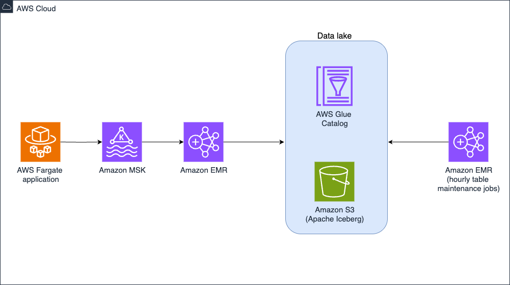
In our previous post Backtesting index rebalancing arbitrage with Amazon EMR and Apache Iceberg, we showed how to use Apache Iceberg in the context of strategy backtesting. In this post, we focus on data management implementation options such as accessing data directly in Amazon Simple Storage Service (Amazon S3), using popular data formats like Parquet, or using open table formats like Iceberg. Our experiments are based on real-world historical full order book data, provided by our partner CryptoStruct, and compare the trade-offs between these choices, focusing on performance, cost, and quant developer productivity.
Data management is the foundation of quantitative research. Quant researchers spend approximately 80% of their time on necessary but not impactful data management tasks such as data ingestion, validation, correction, and reformatting. Traditional data management choices include relational, SQL, NoSQL, and specialized time series databases. In recent years, advances in parallel computing in the cloud have made object stores like Amazon S3 and columnar file formats like Parquet a preferred choice.
This post explores how Iceberg can enhance quant research platforms by improving query performance, reducing costs, and increasing productivity, ultimately enabling faster and more efficient strategy development in quantitative finance. Our analysis shows that Iceberg can accelerate query performance by up to 52%, reduce operational costs, and significantly improve data management at scale.
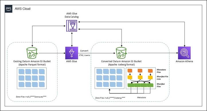
Having chosen Amazon S3 as our storage layer, a key decision is whether to access Parquet files directly or use an open table format like Iceberg. Iceberg offers distinct advantages through its metadata layer over Parquet, such as improved data management, performance optimization, and integration with various query engines.
In this post, we use the term vanilla Parquet to refer to Parquet files stored directly in Amazon S3 and accessed through standard query engines like Apache Spark, without the additional features provided by table formats such as Iceberg.
Quant developer and researcher productivity
In this section, we focus on the productivity features offered by Iceberg and how it compares to directly reading files in Amazon S3. As mentioned earlier, 80% of quantitative research work is attributed to data management tasks. Business impact heavily relies on quality data (“garbage in, garbage out”). Quants and platform teams have to ingest data from multiple sources with different velocities and update frequencies, and then validate and correct the data. These activities translate into the ability to run append, insert, update, and delete operations. For simple append operations, both Parquet on Amazon S3 and Iceberg offer similar convenience and productivity. However, real-world data is never perfect and needs to be corrected. Gaps filling (inserts), error corrections and restatements (updates), and removing duplicates (deletes) are the most obvious examples. When writing data in the Parquet format directly to Amazon S3 without using an open table format like Iceberg, you have to write code to identify the affected partition, correct errors, and rewrite the partition. Moreover, if the write job fails or a downstream read job occurs during this write operation, all downstream jobs have the possibility of reading inconsistent data. However, Iceberg has built-in insert, update, and delete features with ACID (Atomicity, Consistency, Isolation, Durability) properties, and the framework itself manages the Amazon S3 mechanics on your behalf.
Guarding against lookahead bias is an essential capability of any quant research platform—what backtests as a profitable trading strategy can render itself useless and unprofitable in real time. Iceberg provides time travel and snapshotting capabilities out of the box to manage lookahead bias that could be embedded in the data (such as delayed data delivery).
Simplified data corrections and updates
Iceberg enhances data management for quants in capital markets through its robust insert, delete, and update capabilities. These features allow efficient data corrections, gap-filling in time series, and historical data updates without disrupting ongoing analyses or compromising data integrity.
Unlike direct Amazon S3 access, Iceberg supports these operations on petabyte-scale data lakes without requiring complex custom code. This simplifies data modification processes, which is crucial for ingesting and updating large volumes of market and trade data, quickly iterating on backtesting and reprocessing workflows, and maintaining detailed audit trails for risk and compliance requirements.
Iceberg’s table format separates data files from metadata files, enabling efficient data modifications without full dataset rewrites. This approach also reduces expensive ListObjects API calls typically needed when directly accessing Parquet files in Amazon S3.
Additionally, Iceberg offers merge on read (MoR) and copy on write (CoW) approaches, providing flexibility for different quant research needs. MoR enables faster writes, suitable for frequently updated datasets, and CoW provides faster reads, beneficial for read-heavy workflows like backtesting.
For example, when a new data source or attribute is added, quant researchers can seamlessly incorporate it into their Iceberg tables and then reprocess historical data, confident they’re using correct, time-appropriate information. This capability is particularly valuable in maintaining the integrity of backtests and the reliability of trading strategies.
In scenarios involving large-scale data corrections or updates, such as adjusting for stock splits or dividend payments across historical data, Iceberg’s efficient update mechanisms significantly reduce processing time and resource usage compared to traditional methods.
These features collectively improve productivity and data management efficiency in quant research environments, allowing researchers to focus more on strategy development and less on data handling complexities.
Historical data access for backtesting and validation
Iceberg’s time travel feature can enable quant developers and researchers to access and analyze historical snapshots of their data. This capability can be useful while performing tasks like backtesting, model validation, and understanding data lineage.
Iceberg simplifies time travel workflows on Amazon S3 by introducing a metadata layer that tracks the history of changes made to the table. You can refer to this metadata layer to create a mental model of how Iceberg’s time travel capability works.
Iceberg’s time travel capability is driven by a concept called snapshots, which are recorded in metadata files. These metadata files act as a central repository that stores table metadata, including the history of snapshots. Additionally, Iceberg uses manifest files to provide a representation of data files, their partitions, and any associated deleted files. These manifest files are referenced in the metadata snapshots, allowing Iceberg to identify the relevant data for a specific point in time.
When a user requests a time travel query, the typical workflow involves querying a specific snapshot. Iceberg uses the snapshot identifier to locate the corresponding metadata snapshot in the metadata files. The time travel capability is invaluable to quants, enabling them to backtest and validate strategies against historical data, reproduce and debug issues, perform what-if analysis, comply with regulations by maintaining audit trails and reproducing past states, and roll back and recover from data corruption or errors. Quants can also gain deeper insights into current market trends and correlate them with historical patterns. Also, the time travel feature can further mitigate any risks of lookahead bias. Researchers can access the exact data snapshots that were present in the past, and then run their models and strategies against this historical data, without the risk of inadvertently incorporating future information.
Seamless integration with familiar tools
Iceberg provides a variety of interfaces that enable seamless integration with the open source tools and AWS services that quant developers and researchers are familiar with.
Iceberg provides a comprehensive SQL interface that allows quant teams to interact with their data using familiar SQL syntax. This SQL interface is compatible with popular query engines and data processing frameworks, such as Spark, Trino, Amazon Athena, and Hive. Quant developers and researchers can use their existing SQL knowledge and tools to query, filter, aggregate, and analyze their data stored in Iceberg tables.
In addition to the primary interface of SQL, Iceberg also provides the DataFrame API, which allows quant teams to programmatically interact with their data with popular distributed data processing frameworks like Spark and Flink as well as thin clients like PyIceberg. Quants can further use this API to build more programmatic approaches to access and manipulate data, allowing for the implementation of custom logic and integration of Iceberg with other AWS ecosystems like Amazon EMR.
Although accessing data from Amazon S3 is a viable option, Iceberg provides several advantages like metadata management, performance optimization using partition pruning, data manipulation, and a rich AWS ecosystem integration including services like Athena and Amazon EMR with more seamless and feature-rich data processing experience.
Undifferentiated heavy lifting
Data partitioning is one of major contributing factors to optimizing aggregate throughput to and from Amazon S3, contributing to overall High Performance Computing (HPC) environment price-performance.
Quant researchers often face performance bottlenecks and complex data management challenges when dealing with large-scale datasets in Amazon S3. As discussed in Best practices design patterns: optimizing Amazon S3 performance, single prefix performance is limited to 3,500 PUT/COPY/POST/DELETE or 5,500 GET/HEAD requests per second per partitioned Amazon S3 prefix. Iceberg’s metadata layer and intelligent partitioning strategies automatically optimize data access patterns, reducing the likelihood of I/O throttling and minimizing the need for manual performance tuning. This automation allows quant teams to focus on developing and refining trading strategies rather than troubleshooting data access issues or optimizing storage layouts.
In this section, we discuss situations we discovered while running our experiments at scale and solutions provided by Iceberg vs. vanilla Parquet when accessing data in Amazon S3.
As we mentioned in the introduction, the nature of quant research is “fail fast”—new ideas have to be quickly evaluated and then either prioritized for a deep dive or dismissed. This makes it impossible to come up with universal partitioning that works all the time and for all research styles.
When accessing data directly as Parquet files in Amazon S3, without using an open table format like Iceberg, partitioning and throttling issues can arise. Partitioning in this case is determined by the physical layout of files in Amazon S3, and a mismatch between the intended partitioning and the actual file layout can lead to I/O throttling exceptions. Additionally, listing directories in Amazon S3 can also result in throttling exceptions due to the high number of API calls required.
In contrast, Iceberg provides a metadata layer that abstracts away the physical file layout in Amazon S3. Partitioning is defined at the table level, and Iceberg handles the mapping between logical partitions and the underlying file structure. This abstraction helps mitigate partitioning issues and reduces the likelihood of I/O throttling exceptions. Furthermore, Iceberg’s metadata caching mechanism minimizes the number of List API calls required, addressing the directory listing throttling issue.
Although both approaches involve direct access to Amazon S3, Iceberg is an open table format that introduces a metadata layer, providing better partitioning management and reducing the risk of throttling exceptions. It doesn’t act as a database itself, but rather as a data format and processing engine on top of the underlying storage (in this case, Amazon S3).
One of the most effective techniques to address Amazon S3 API quota limits is salting (random hash prefixes)—a method that adds random partition IDs to Amazon S3 paths. This increases the probability of prefixes residing on different physical partitions, helping distribute API requests more evenly. Iceberg supports this functionality out of the box for both data ingestion and reading.
Implementing salting directly in Amazon S3 requires complex custom code to create and use partitioning schemes with random keys in the naming hierarchy. This approach necessitates a custom data catalog and metadata system to map physical paths to logical paths, allowing direct partition access without relying on Amazon S3 List API calls. Without such a system, applications risk exceeding Amazon S3 API quotas when accessing specific partitions.
At petabyte scale, Iceberg’s advantages become clear. It efficiently manages data through the following features:
- Directory caching
- Configurable partitioning strategies (range, bucket)
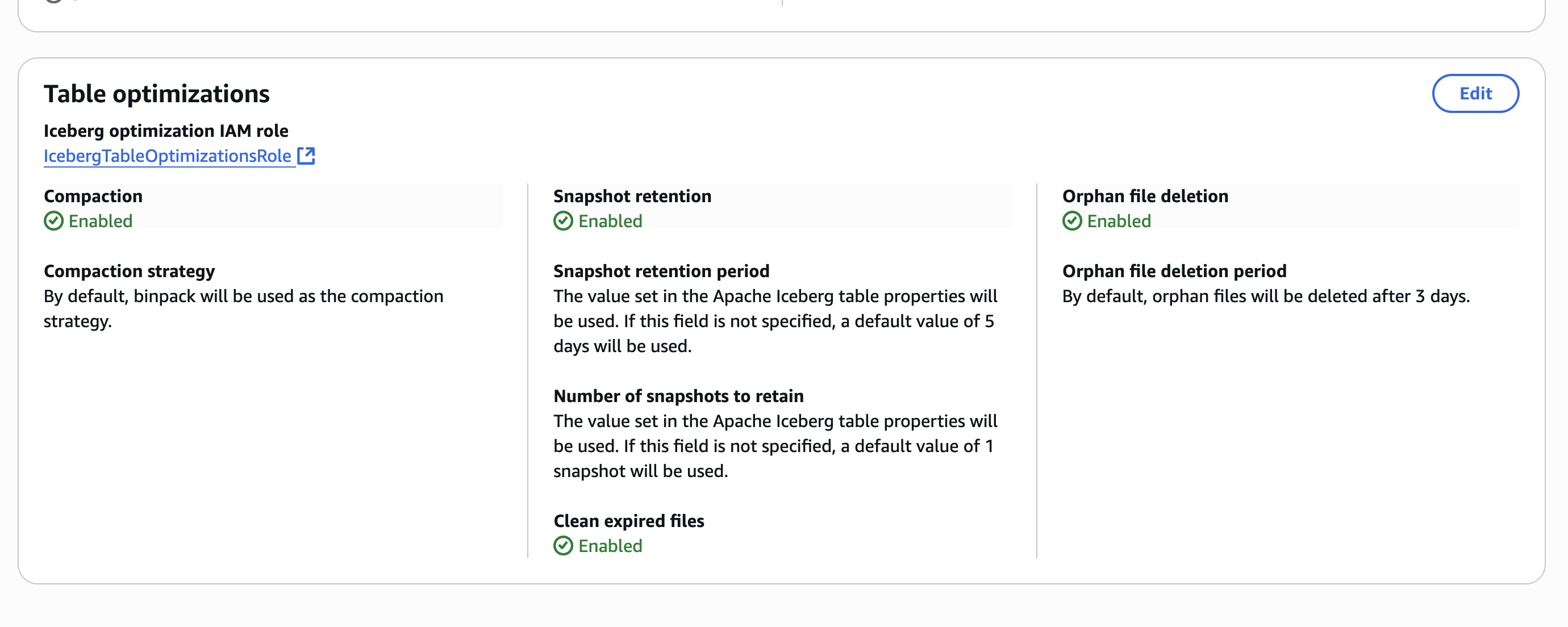
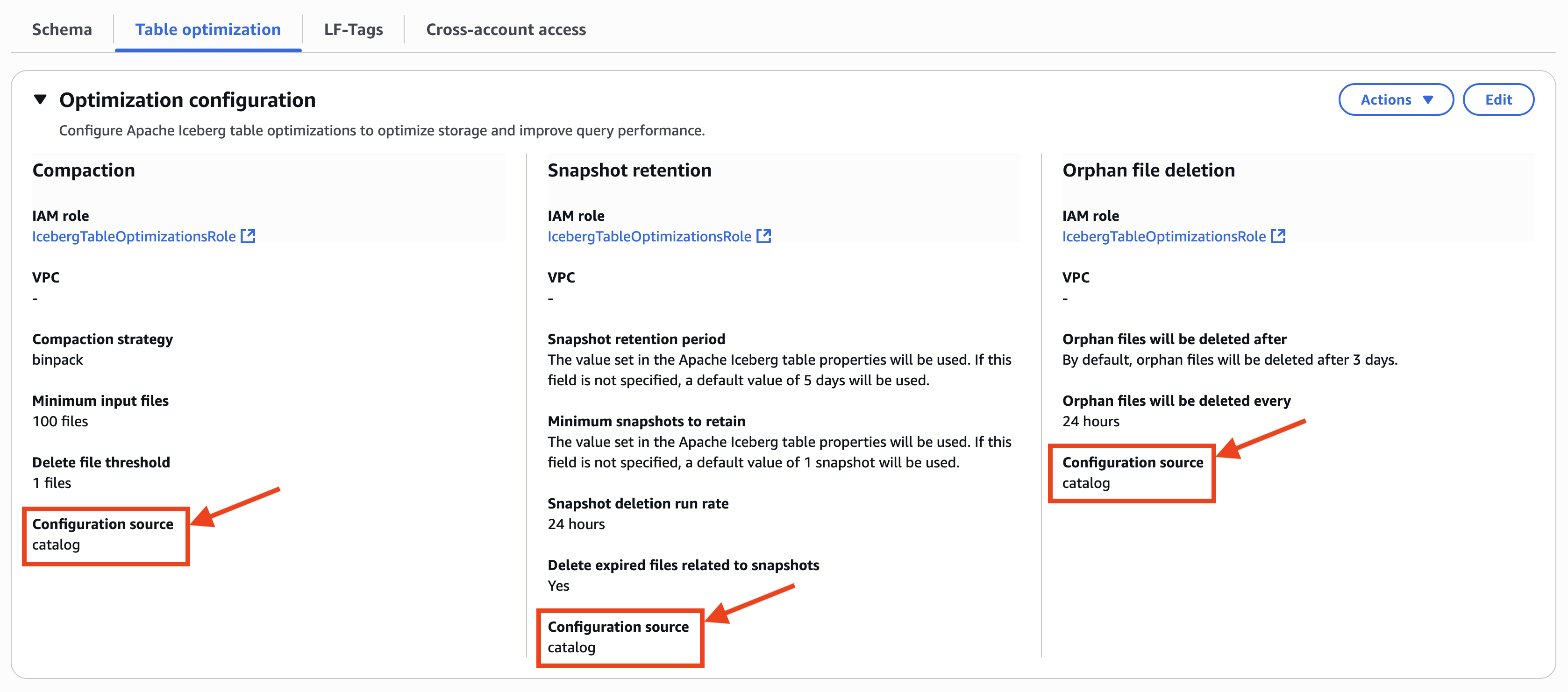
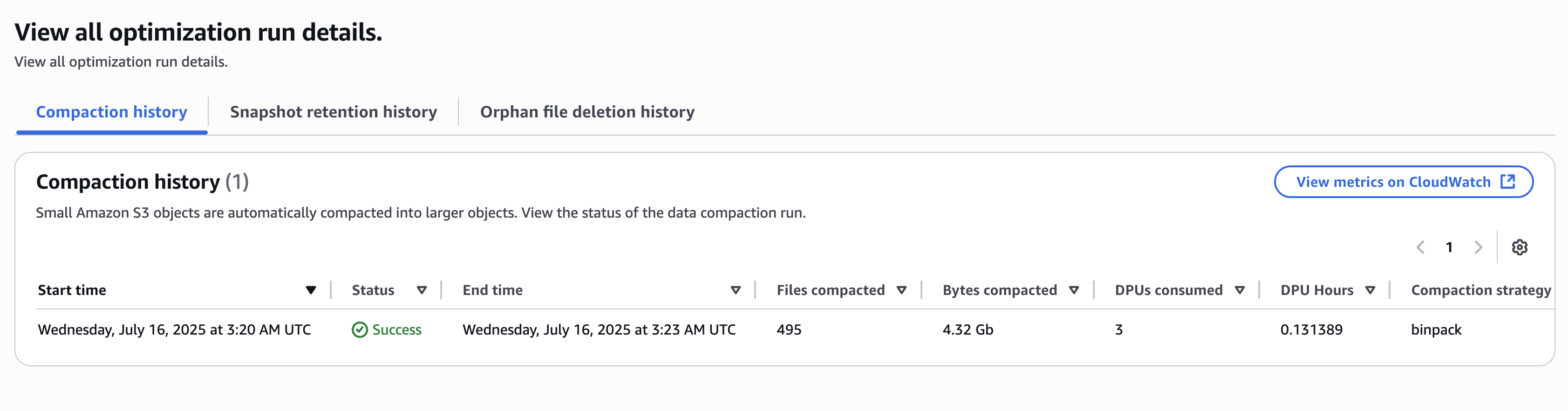
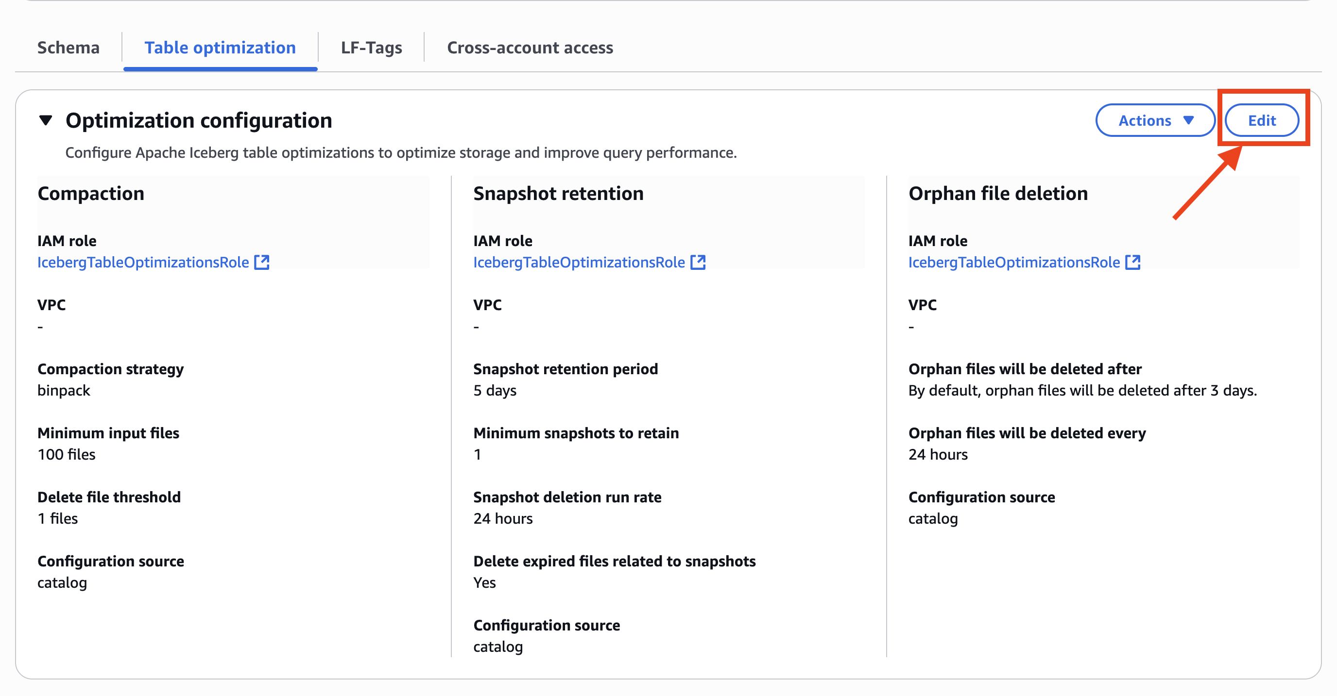
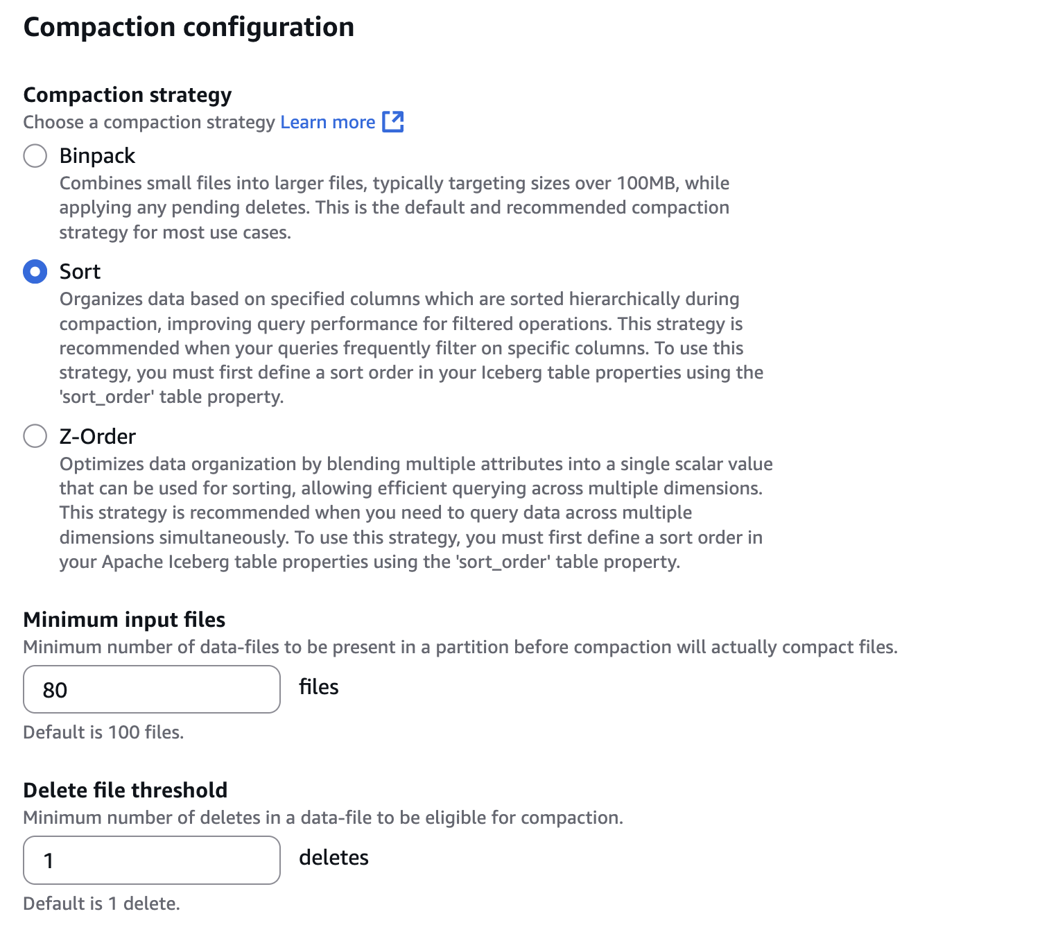
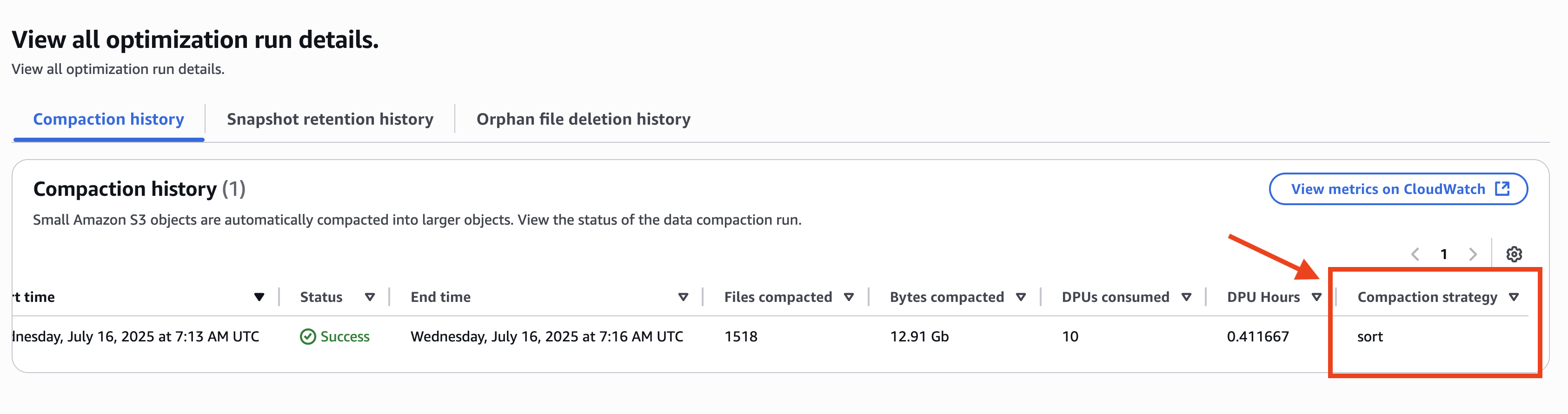
- Data management functionality (compaction)
- Catalog, metadata, and statistics use for optimal execution plans
These built-in features eliminate the need for custom solutions to manage Amazon S3 API quotas and data organization at scale, reducing development time and maintenance costs while improving query performance and reliability.
Performance
We highlighted a lot of the functionality of Iceberg that eliminates undifferentiated heavy lifting and improves developer and quant productivity. What about performance?
This section evaluates whether Iceberg’s metadata layer introduces overhead or delivers optimization for quantitative research use cases, comparing it with vanilla Parquet access on Amazon S3. We examine how these approaches impact common quant research queries and workflows.
The key question is whether Iceberg’s metadata layer, designed to optimize vanilla Parquet access on Amazon S3, introduces overhead or delivers the intended optimization for quantitative research use cases. Then we discuss overlapping optimization techniques, such as data distribution and sorting. We also discuss that there is no magic partitioning and all sorting scheme where one size fits all in the context of quant research. Our benchmarks show that Iceberg performs comparably to direct Amazon S3 access, with additional optimizations from its metadata and statistics usage, similar to database indexing.
Vanilla Parquet vs Iceberg: Amazon S3 read performance
We created four different datasets: two using Iceberg and two with direct Amazon S3 Parquet access, each with both sorted and unsorted write distributions. The purpose of this exercise was to compare the performance of direct Amazon S3 Parquet access vs. the Iceberg open table format, taking into account the impact of write distribution patterns when running various queries commonly used in quantitative trading research.
Query 1
We first run a simple count query to get the total number of records in the table. This query helps understand the baseline performance for a straightforward operation. For example, if the table contains tick-level market data for various financial instruments, the count can give an idea of the total number of data points available for analysis.
The following is the code for vanilla Parquet:
count = spark.read.parquet(s3://example-s3-bucket/path/to/data).count()
The following is the code for Iceberg:
count = spark.read.table(table_name).count()
# We used typical count query for the performance comparision however this could have been also done using metadata as shown below which completes in few seconds
spark.read.format("iceberg").load(f"{table_name}.files").select(sum("record_count")).show(truncate=False)
Query 2
Our second query is a grouping and counting query to find the number of records for each combination of exchange_code and instrument. This query is commonly used in quantitative trading research to analyze market liquidity and trading activity across different instruments and exchanges.
The following is the code for vanilla Parquet:
spark.read.parquet(s3://example-s3-bucket/path/to/data) \
         .groupBy("exchange_code", "instrument") \
         .count() \
         .orderBy("count", ascending=False) \
         .count().show(truncate=False)
The following is the code for Iceberg:
spark.read.table(table_name) \
        .groupBy("exchange_code", "instrument") \
        .count() \
        .orderBy("count", ascending=False) \
        .show(truncate=False)
Query 3
Next, we run a distinct query to retrieve the distinct combinations of year, month, and day from the adapterTimestamp_ts_utc column. In quantitative trading research, this query can be helpful for understanding the time range covered by the dataset. Researchers can use this information to identify periods of interest for their analysis, such as specific market events, economic cycles, or seasonal patterns.
The following is the code for vanilla Parquet:
spark.read.parquet(s3://example-s3-bucket/path/to/data) \
         .select(f.year("adapterTimestamp_ts_utc").alias("year"),
                 f.month("adapterTimestamp_ts_utc").alias("month"),
                 f.dayofmonth("adapterTimestamp_ts_utc").alias("day")) \
         .distinct() \
         .count() \
         .show(truncate=False)
The following is the code for Iceberg:
spark.read.table(table_name) \
        .select(f.year("adapterTimestamp_ts_utc").alias("year"),
                f.month("adapterTimestamp_ts_utc").alias("month"),
                f.dayofmonth("adapterTimestamp_ts_utc").alias("day")) \
        .distinct() \
        .count() \
        .show(truncate=False)
Query 4
Lastly, we run a grouping and counting query with a date range filter on the adapterTimestamp_ts_utc column. This query is similar to Query 2 but focuses on a specific time period. You could use this query to analyze market activity or liquidity during specific time periods, such as periods of high volatility, market crashes, or economic events. Researchers can use this information to identify potential trading opportunities or investigate the impact of these events on market dynamics.
The following is the code for vanilla Parquet:
spark.read.parquet(s3://example-s3-bucket/path/to/data) \
         .filter((f.col("adapterTimestamp_ts_utc") >= "2023-04-17 00:00:00") &
                 (f.col("adapterTimestamp_ts_utc") <= "2023-04-18 23:59:59.999")) \
         .groupBy("exchange_code", "instrument") \
         .count() \
         .orderBy("count", ascending=False) \
         .show(truncate=False)
The following is the code for Iceberg. Because Iceberg has a metadata layer, the row count can be fetched from metadata:
spark.read.table(table_name) \
        .filter((f.col("adapterTimestamp_ts_utc") >= "2023-04-17 00:00:00") &
                (f.col("adapterTimestamp_ts_utc") <= "2023-04-18 23:59:59.999")) \
        .groupBy("exchange_code", "instrument") \
        .count() \
        .orderBy("count", ascending=False) \
        .show(truncate=False)
Test results
To evaluate the performance and cost benefits of using Iceberg for our quant research data lake, we created four different datasets: two with Iceberg tables and two with direct Amazon S3 Parquet access, each using both sorted and unsorted write distributions. We first ran AWS Glue write jobs to create the Iceberg tables and then mirrored the same write processes for the Amazon S3 Parquet datasets. For the unsorted datasets, we partitioned the data by exchange and instrument, and for the sorted datasets, we added a sort key on the time column.
Next, we ran a series of queries commonly used in quantitative trading research, including simple count queries, grouping and counting, distinct value queries, and queries with date range filters. Our benchmarking process involved reading data from Amazon S3, performing various transformations and joins, and writing the processed data back to Amazon S3 as Parquet files.
By comparing runtimes and costs across different data formats and write distributions, we quantified the benefits of Iceberg’s optimized data organization, metadata management, and efficient Amazon S3 data handling. The results showed that Iceberg not only enhanced query performance without introducing significant overhead, but also reduced the likelihood of task failures, reruns, and throttling issues, leading to more stable and predictable job execution, particularly with large datasets stored in Amazon S3.
AWS Glue write jobs
In the following table, we compare the performance and the cost implications of using Iceberg vs. vanilla Parquet access on Amazon S3, taking into account the following use cases:
- Iceberg table (unsorted) – We created an Iceberg table partitioned by
exchange_code and instrument This means that the data was physically partitioned in Amazon S3 based on the unique combinations of exchange_code and instrument values. Partitioning the data in this way can improve query performance, because Iceberg can prune out partitions that aren’t relevant to a particular query, reducing the amount of data that needs to be scanned. The data was not sorted on any column in this case, which is the default behavior.
- Vanilla Parquet (unsorted) – For this use case, we wrote the data directly as Parquet files to Amazon S3, without using Iceberg. We repartitioned the data by
exchange_code and instrument columns using standard hash partitioning before writing it out. Repartitioning was necessary to avoid potential throttling issues when reading the data later, because accessing data directly from Amazon S3 without intelligent partitioning can lead to too many requests hitting the same S3 prefix. Like the Iceberg table, the data was not sorted on any column in this case. To make comparison fair, we used the exact repartition count that Iceberg uses.
- Iceberg table (sorted) – We created another Iceberg table, this time partitioned by
exchange_code and instrument Additionally, we sorted the data in this table on the adapterTimestamp_ts_utc column. Sorting the data can improve query performance for certain types of queries, such as those that involve range filters or ordered outputs. Iceberg automatically handles the sorting and partitioning of the data transparently to the user.
- Vanilla Parquet (sorted) – For this use case, we again wrote the data directly as Parquet files to Amazon S3, without using Iceberg. We repartitioned the data by range on the
exchange_code, instrument, and adapterTimestamp_ts_utc columns before writing it out using standard range partitioning with 1996 partition count, because this was what Iceberg was using based on SparkUI. Repartitioning on the time column (adapterTimestamp_ts_utc) was necessary to achieve a sorted write distribution, because Parquet files are sorted within each partition. This sorted write distribution can improve query performance for certain types of queries, similar to the sorted Iceberg table.
| Write Distribution Pattern |
Iceberg Table (Unsorted) |
Vanilla Parquet (Unsorted) |
Iceberg Table (Sorted) |
Vanilla Parquet
(Sorted) |
| DPU Hours |
899.46639 |
915.70222 |
1402 |
1365 |
| Number of S3 Objects |
7444 |
7288 |
9283 |
9283 |
| Size of S3 Parquet Objects |
567.7 GB |
629.8 GB |
525.6 GB |
627.1 GB |
| Runtime |
1h 51m 40s |
1h 53m 29s |
2h 52m 7s |
2h 47m 36s |
AWS Glue read jobs
For the AWS Glue read jobs, we ran a series of queries commonly used in quantitative trading research, such as simple counts, grouping and counting, distinct value queries, and queries with date range filters. We compared the performance of these queries between the Iceberg tables and the vanilla Parquet files read in Amazon S3. In the following table, you can see two AWS Glue jobs that show the performance and cost implications of access patterns described earlier.
| Read Queries / Runtime in Seconds |
Iceberg Table |
Vanilla Parquet |
| COUNT(1) on unsorted |
35.76s |
74.62s |
| GROUP BY and ORDER BY on unsorted |
34.29s |
67.99s |
| DISTINCT and SELECT on unsorted |
51.40s |
82.95s |
| FILTER and GROUP BY and ORDER BY on unsorted |
25.84s |
49.05s |
| COUNT(1) on sorted |
15.29s |
24.25s |
| GROUP BY and ORDER BY on sorted |
15.88s |
28.73s |
| DISTINCT and SELECT on sorted |
30.85s |
42.06s |
| FILTER and GROUP BY and ORDER BY on sorted |
15.51s |
31.51s |
| AWS Glue DPU hours |
45.98 |
67.97 |
Test results insights
These test results offered the following insights:
- Accelerated query performance – Iceberg improved read operations by up to 52% for unsorted data and 51% for sorted data. This speed boost enables quant researchers to analyze larger datasets and test trading strategies more rapidly. In quantitative finance, where speed is crucial, this performance gain allows teams to uncover market insights faster, potentially gaining a competitive edge.
- Reduced operational costs – For read-intensive workloads, Iceberg reduced DPU hours by 32.4% and achieved a 10–16% reduction in Amazon S3 storage. These efficiency gains translate to cost savings in data-intensive quant operations. With Iceberg, firms can run more comprehensive analyses within the same budget or reallocate resources to other high-value activities, optimizing their research capabilities.
- Enhanced data management and scalability – Iceberg showed comparable write performance for unsorted data (899.47 DPU hours vs. 915.70 for vanilla Parquet) and maintained consistent object counts across sorted and unsorted scenarios (7,444 and 9,283, respectively). This consistency leads to more reliable and predictable job execution. For quant teams dealing with large-scale datasets, this reduces time spent on troubleshooting data infrastructure issues and increases focus on developing trading strategies.
- Improved productivity – Iceberg outperformed vanilla Parquet access across various query types. Simple counts were 52.1% faster, grouping and ordering operations improved by 49.6%, and filtered queries were 47.3% faster for unsorted data. This performance enhancement boosts productivity in quant research workflows. It reduces query completion times, allowing quant developers and researchers to spend more time on model development and market analysis, leading to faster iteration on trading strategies.
Conclusion
Quant research platforms often avoid adopting new data management solutions like Iceberg, fearing performance penalties and increased costs. Our analysis disproves these concerns, demonstrating that Iceberg not only matches or enhances performance compared to direct Amazon S3 access, but also provides substantial additional benefits.
Our tests reveal that Iceberg significantly accelerates query performance, with improvements of up to 52% for unsorted data and 51% for sorted data. This speed boost enables quant researchers to analyze larger datasets and test trading strategies more rapidly, potentially uncovering valuable market insights faster.
Iceberg streamlines data management tasks, allowing researchers to focus on strategy development. Its robust insert, update, and delete capabilities, combined with time travel features, enable effortless management of complex datasets, improving backtest accuracy and facilitating rapid strategy iteration.
The platform’s intelligent handling of partitioning and Amazon S3 API quota issues eliminates undifferentiated heavy lifting, freeing quant teams from low-level data engineering tasks. This automation redirects efforts to high-value activities such as model development and market analysis. Moreover, our tests show that for read-intensive workloads, Iceberg reduced DPU hours by 32.4% and achieved a 10–16% reduction in Amazon S3 storage, leading to significant cost savings.
Flexibility is a key advantage of Iceberg. Its various interfaces, including SQL, DataFrames, and programmatic APIs, integrate seamlessly with existing quant research workflows, accommodating diverse analysis needs and coding preferences.
By adopting Iceberg, quant research teams gain both performance enhancements and powerful data management tools. This combination creates an environment where researchers can push analytical boundaries, maintain high data integrity standards, and focus on generating valuable insights. The improved productivity and reduced operational costs enable quant teams to allocate resources more effectively, ultimately leading to a more competitive edge in quantitative finance.
About the Authors
 Guy Bachar is a Senior Solutions Architect at AWS based in New York. He specializes in assisting capital markets customers with their cloud transformation journeys. His expertise encompasses identity management, security, and unified communication.
 Sercan Karaoglu is Senior Solutions Architect, specialized in capital markets. He is a former data engineer and passionate about quantitative investment research.
Boris Litvin is a Principal Solutions Architect at AWS. His job is in financial services industry innovation. Boris joined AWS from the industry, most recently Goldman Sachs, where he held a variety of quantitative roles across equity, FX, and interest rates, and was CEO and Founder of a quantitative trading FinTech startup.
Salim Tutuncu is a Senior Partner Solutions Architect Specialist on Data & AI, based in Dubai with a focus on the EMEA. With a background in the technology sector that spans roles as a data engineer, data scientist, and machine learning engineer, Salim has built a formidable expertise in navigating the complex landscape of data and artificial intelligence. His current role involves working closely with partners to develop long-term, profitable businesses using the AWS platform, particularly in data and AI use cases.
Alex Tarasov is a Senior Solutions Architect working with Fintech startup customers, helping them to design and run their data workloads on AWS. He is a former data engineer and is passionate about all things data and machine learning.
Jiwan Panjiker is a Solutions Architect at Amazon Web Services, based in the Greater New York City area. He works with AWS enterprise customers, helping them in their cloud journey to solve complex business problems by making effective use of AWS services. Outside of work, he likes spending time with his friends and family, going for long drives, and exploring local cuisine.
 Tomohiro Tanaka is a Senior Cloud Support Engineer at Amazon Web Services (AWS). He’s passionate about helping customers use Apache Iceberg for their data lakes on AWS. In his free time, he enjoys a coffee break with his colleagues and making coffee at home.
 Noritaka Sekiyama is a Principal Big Data Architect with AWS Analytics services. He’s responsible for building software artifacts to help customers. In his spare time, he enjoys cycling on his road bike.
 Sandeep Adwankar is a Senior Product Manager at Amazon Web Services (AWS). Based in the California Bay Area, he works with customers around the globe to translate business and technical requirements into products customers can use to improve how they manage, secure, and access data.
 Siddharth Padmanabhan Ramanarayanan is a Senior Software Engineer on the AWS Glue and AWS Lake Formation team, where he focuses on building scalable distributed systems for data analytics workloads. He is passionate about helping customers optimize their cloud infrastructure for performance and cost efficiency.


 Guy Bachar is a Senior Solutions Architect at AWS based in New York. He specializes in assisting capital markets customers with their cloud transformation journeys. His expertise encompasses identity management, security, and unified communication.
 Sercan Karaoglu is Senior Solutions Architect, specialized in capital markets. He is a former data engineer and passionate about quantitative investment research.
 Boris Litvin is a Principal Solutions Architect at AWS. His job is in financial services industry innovation. Boris joined AWS from the industry, most recently Goldman Sachs, where he held a variety of quantitative roles across equity, FX, and interest rates, and was CEO and Founder of a quantitative trading FinTech startup.
 Salim Tutuncu is a Senior Partner Solutions Architect Specialist on Data & AI, based in Dubai with a focus on the EMEA. With a background in the technology sector that spans roles as a data engineer, data scientist, and machine learning engineer, Salim has built a formidable expertise in navigating the complex landscape of data and artificial intelligence. His current role involves working closely with partners to develop long-term, profitable businesses using the AWS platform, particularly in data and AI use cases.
 Alex Tarasov is a Senior Solutions Architect working with Fintech startup customers, helping them to design and run their data workloads on AWS. He is a former data engineer and is passionate about all things data and machine learning.
 Jiwan Panjiker is a Solutions Architect at Amazon Web Services, based in the Greater New York City area. He works with AWS enterprise customers, helping them in their cloud journey to solve complex business problems by making effective use of AWS services. Outside of work, he likes spending time with his friends and family, going for long drives, and exploring local cuisine.


 Navnit Shukla serves as an AWS Specialist Solutions Architect with a focus on Analytics. He possesses a strong enthusiasm for assisting clients in discovering valuable insights from their data. Through his expertise, he constructs innovative solutions that empower businesses to arrive at informed, data-driven choices. Notably, Navnit Shukla is the accomplished author of the book titled Data Wrangling on AWS. He can be reached through
  Angel Conde Manjon is a Sr. PSA Specialist on Data & AI, based in Madrid, and focuses on EMEA South and Israel. He has previously worked on research related to data analytics and artificial intelligence in diverse European research projects. In his current role, Angel helps partners develop businesses centered on data and AI.
 Amit Singh currently serves as a Senior Solutions Architect at AWS, specializing in analytics and IoT technologies. With extensive expertise in designing and implementing large-scale distributed systems, Amit is passionate about empowering clients to drive innovation and achieve business transformation through AWS solutions.
 Sandeep Adwankar is a Senior Technical Product Manager at AWS. Based in the California Bay Area, he works with customers around the globe to translate business and technical requirements into products that enable customers to improve how they manage, secure, and access data.


 Sotaro Hikita is a Solutions Architect. He supports customers in a wide range of industries, especially the financial industry, to build better solutions. He is particularly passionate about big data technologies and open source software.


 Shaheer Mansoor is a Senior Machine Learning Engineer at AWS, where he specializes in developing cutting-edge machine learning platforms. His expertise lies in creating scalable infrastructure to support advanced AI solutions. His focus areas are MLOps, feature stores, data lakes, model hosting, and generative AI.
 Anoop Kumar K M is a Data Architect at AWS with focus in the data and analytics area. He helps customers in building scalable data platforms and in their enterprise data strategy. His areas of interest are data platforms, data analytics, security, file systems and operating systems. Anoop loves to travel and enjoys reading books in the crime fiction and financial domains.
 Sreenivas Nettem is a Lead Database Consultant at AWS Professional Services. He has experience working with Microsoft technologies with a specialization in SQL Server. He works closely with customers to help migrate and modernize their databases to AWS.


 Sandeep Adwankar is a Senior Product Manager at AWS. Based in the California Bay Area, he works with customers around the globe to translate business and technical requirements into products that enable customers to improve how they manage, secure, and access data.
 Srividya Parthasarathy is a Senior Big Data Architect on the AWS Lake Formation team. She enjoys building data mesh solutions and sharing them with the community.
 Paul Villena is a Senior Analytics Solutions Architect in AWS with expertise in building modern data and analytics solutions to drive business value. He works with customers to help them harness the power of the cloud. His areas of interests are infrastructure as code, serverless technologies, and coding in Python.
 Carlos Rodrigues is a Big Data Specialist Solutions Architect at AWS. He helps customers worldwide build transactional data lakes on AWS using open table formats like Apache Iceberg and Apache Hudi. He can be reached via
  Imtiaz (Taz) Sayed is the WW Tech Leader for Analytics at AWS. He is an expert on data engineering and enjoys engaging with the community on all things data and analytics. He can be reached via
  Shana Schipers is an Analytics Specialist Solutions Architect at AWS, focusing on big data. She supports customers worldwide in building transactional data lakes using open table formats like Apache Hudi, Apache Iceberg, and Delta Lake on AWS.


 Rajdip Chaudhuri is a Senior Solutions Architect with Amazon Web Services specializing in data and analytics. He enjoys working with AWS customers and partners on data and analytics requirements. In his spare time, he enjoys soccer and movies.


 Avijit Goswami is a Principal Solutions Architect at AWS specialized in data and analytics. He supports AWS strategic customers in building high-performing, secure, and scalable data lake solutions on AWS using AWS managed services and open-source solutions. Outside of his work, Avijit likes to travel, hike, watch sports, and listen to music.
 Rajarshi Sarkar is a Software Development Engineer at Amazon EMR/Athena. He works on cutting-edge features of Amazon EMR/Athena and is also involved in open-source projects such as Apache Iceberg and Trino. In his spare time, he likes to travel, watch movies, and hang out with friends.


 Ranjit Rajan is a Principal Data Lab Solutions Architect with AWS. Ranjit works with AWS customers to help them design and build data and analytics applications in the cloud.
 Kannan Iyer is a Senior Data Lab Solutions Architect with AWS. Kannan works with AWS customers to help them design and build data and analytics applications in the cloud.
 Alexandre Rezende is a Data Lab Solutions Architect with AWS. Alexandre works with customers on their Business Intelligence, Data Warehouse, and Data Lake use cases, design architectures to solve their business problems, and helps them build MVPs to accelerate their path to production.
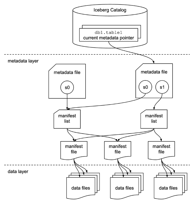


 Flora Wu is a Sr. Resident Architect at AWS Data Lab. She helps enterprise customers create data analytics strategies and build solutions to accelerate their businesses outcomes. In her spare time, she enjoys playing tennis, dancing salsa, and traveling.
 Daniel Li is a Sr. Solutions Architect at Amazon Web Services. He focuses on helping customers develop, adopt, and implement cloud services and strategy. When not working, he likes spending time outdoors with his family.


 Dhiraj Thakur is a Solutions Architect with Amazon Web Services. He works with AWS customers and partners to provide guidance on enterprise cloud adoption, migration, and strategy. He is passionate about technology and enjoys building and experimenting in the analytics and AI/ML space.
 Rajdip Chaudhuri is Solutions Architect with Amazon Web Services specializing in data and analytics. He enjoys working with AWS customers and partners on data and analytics requirements. In his spare time, he enjoys soccer.


 SaiKiran Reddy Aenugu is a Data Architect in the Amazon Web Services (AWS) Data Lab. He has 10 years of experience implementing data loading, transformation, and visualization processes. SaiKiran currently helps organizations in North America to adopt modern data architectures such as data lakes and data mesh. He has experience in the retail, airline, and finance sectors.
 Narendra Merla is a Data Architect in the Amazon Web Services (AWS) Data Lab. He has 12 years of experience in designing and productionalizing both real-time and batch-oriented data pipelines and building data lakes on both cloud and on-premises environments. Narendra currently helps organizations in North America to build and design robust data architectures, and has experience in the telecom and finance sectors.