All posts by Narendra Gupta

Modernize game intelligence with generative AI on Amazon Redshift

Post Syndicated from Narendra Gupta original https://aws.amazon.com/blogs/big-data/modernize-game-intelligence-with-generative-ai-on-amazon-redshift/

Game studios generate massive amounts of player and gameplay telemetry, but transforming that data into meaningful insights is often slow, technical, and dependent on SQL expertise. With the new Amazon Redshift integration for Amazon Bedrock Knowledge Bases, teams can unlock instant, AI-powered analytics by asking questions in natural language. Analysts, product managers, and designers can now explore Amazon Redshift data conversationally—no query writing required—and Amazon Bedrock automatically generates optimized SQL, executes it on Amazon Redshift, and returns clear, actionable answers. This brings together the scale and performance of Amazon Redshift with the intelligence of Amazon Bedrock, enabling faster decisions, deeper player understanding, and more engaging game experiences.

Amazon Redshift can be used as a structured data source for Amazon Bedrock Knowledge Bases, allowing for natural language querying and retrieval of information from Amazon Redshift. Amazon Bedrock Knowledge Bases can transform natural language queries into SQL queries, so users can retrieve data directly from the source without needing to move or preprocess the data. A game analyst can now ask, “How many players completed all the levels in a game?” or “List the top 5 players by the number of times the game was played,” and Amazon Bedrock Knowledge Bases automatically translates that query into SQL, runs the query against Amazon Redshift, and returns the results—or even provides a summarized narrative response.

To generate accurate SQL queries, Amazon Bedrock Knowledge Bases uses database schema, previous query history, and other domain or business knowledge such as table and column annotations that are provided about the data sources. In this post, we discuss some of the best practices to improve accuracy while interacting with Amazon Bedrock using Amazon Redshift as the knowledge base.

Solution overview

In this post, we illustrate the best practices using gaming industry use cases. You will converse with players and their game attempts data in natural language and get the response back in natural language. In the process, you will learn the best practices. To follow along with the use case, follow these high-level steps:

  1. Load game attempts data into the Redshift cluster.
  2. Create a knowledge base in Amazon Bedrock and sync it with the Amazon Redshift data store.
  3. Review the approaches and best practices to improve the accuracy of response from the knowledge base.
  4. Complete the detailed walkthrough for defining and using curated queries to improve the accuracy of responses from the knowledge base.

Prerequisites

To implement the solution, you need to complete the following prerequisites:

Load game attempts and players data

To load the datasets to Amazon Redshift, complete the following steps:

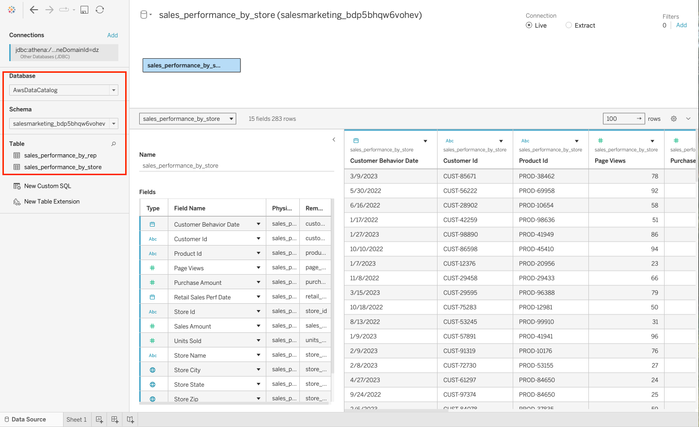
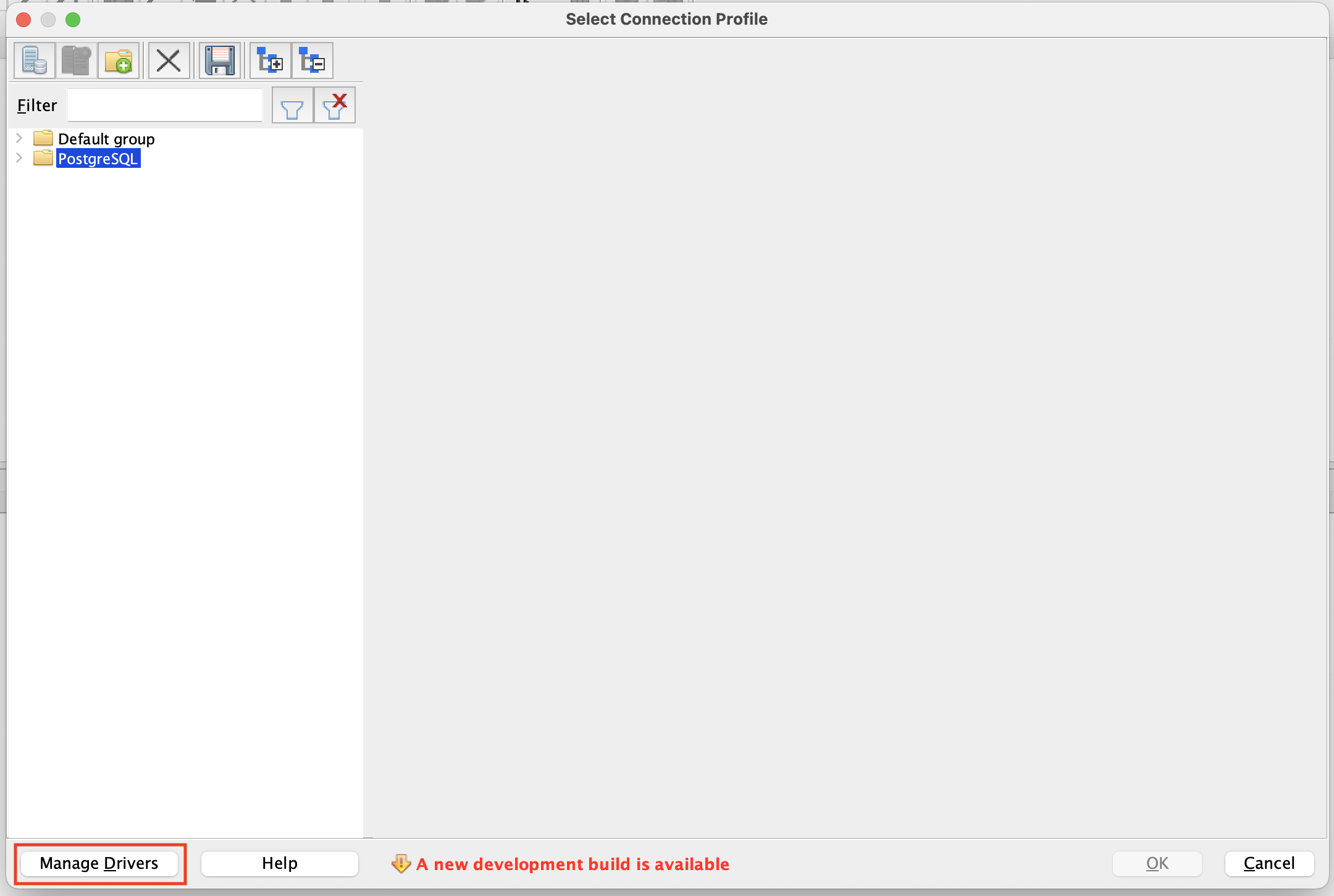
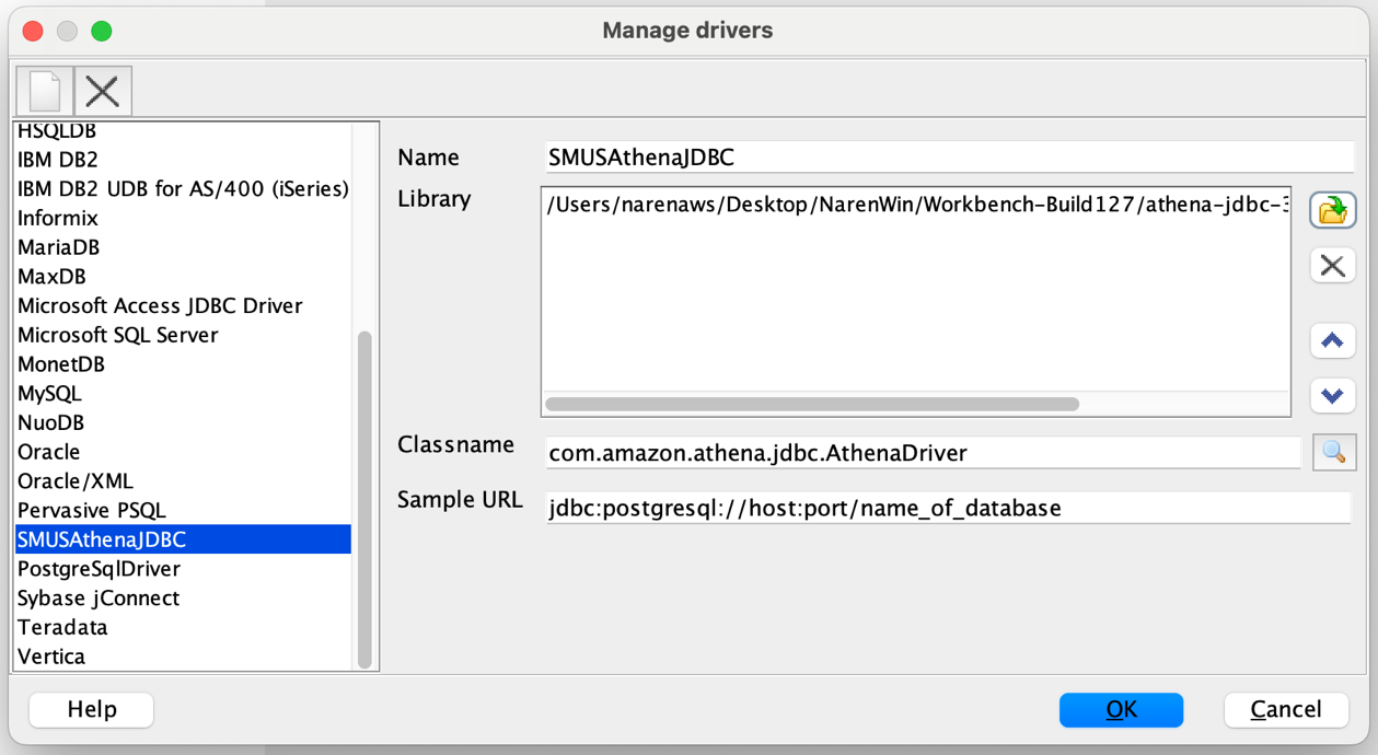
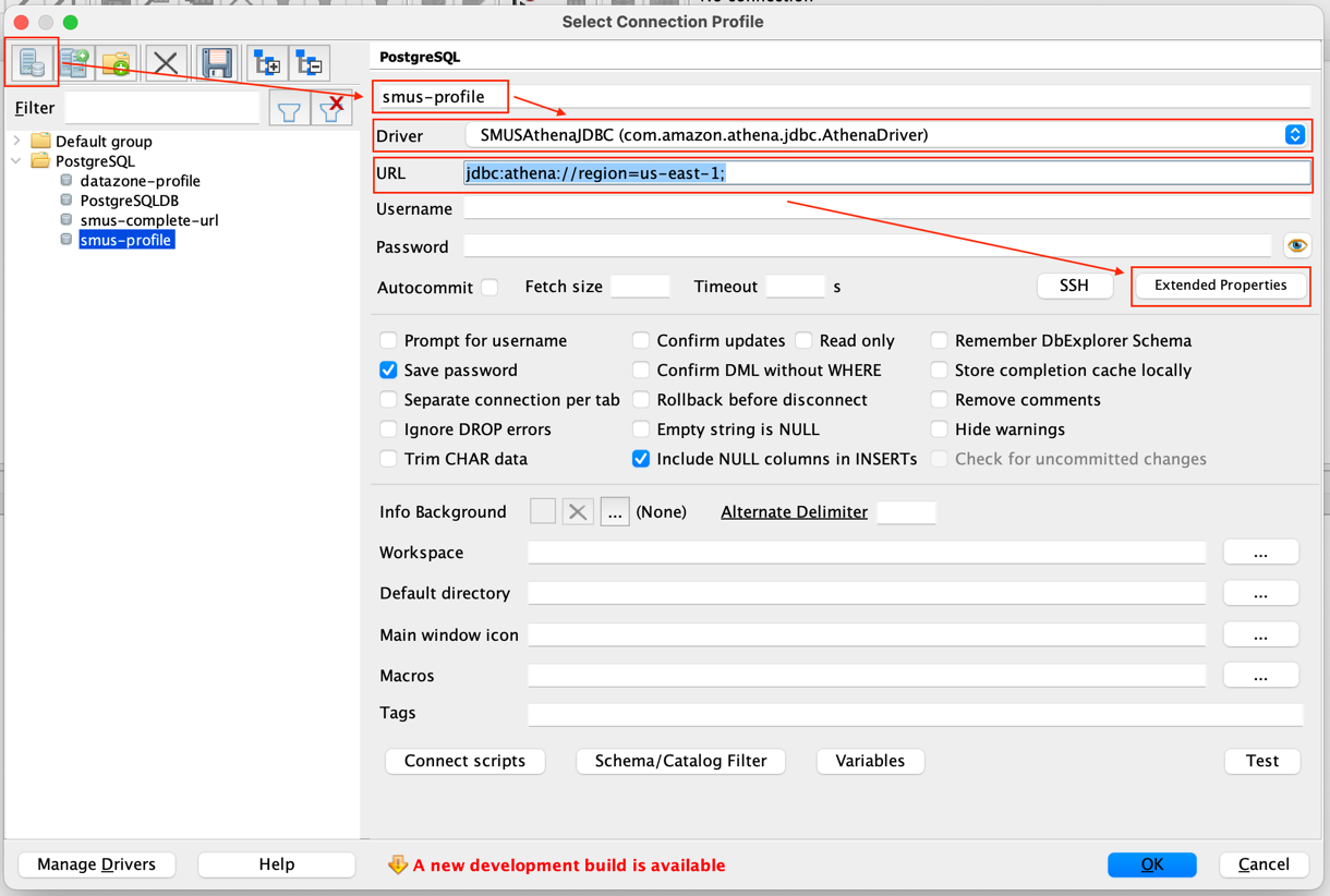
  1. Open Amazon Redshift Query Editor V2 or another SQL editor of your choice and connect to the Redshift database.
  2. Run the following SQL to create the data tables to store games attempts and player details:
    CREATE TABLE game_attempts (
        player_id numeric(10, 0), -- Player ID.
        level_id numeric(5, 0), -- Game level ID
        f_success integer, -- Indicates whether user completed the level (1: completed, 0: fails).
        f_duration real, -- duration of the attempt.  Units in seconds
        f_reststep real, -- The ratio of the remaining steps to the limited steps.  Failure is 0.
        f_help integer, -- Whether extra help, such as props and hints, was used.  1- used, 0- not used
        game_time timestamp, -- Attempt timestamp
        bp_used boolean -- Whether bonus packages used or not.  true: used, false: not used.
    );
    CREATE TABLE players (
    	player_id numeric(10, 0), -- Player ID
    	lost_label boolean, -- Indicated if user retained or lost.  true: lost ,  false: retained
    	bp_category integer -- bonus package category codes
    );

  3. Download the game attempts and players datasets to your local storage.
  4. Create an Amazon Simple Storage Service (Amazon S3) bucket with a unique name. For instructions, refer to Creating a general purpose bucket.
  5. Upload the downloaded files into your newly created S3 bucket.
  6. Using the following COPY command statements, load the datasets from Amazon S3 into the new tables you created in Amazon Redshift. Replace <<your_s3_bucket>> with the name of your S3 bucket and <<your_region>> with your AWS Region:
    COPY game_attempts 
    FROM 's3://<<your_s3_bucket>>/game_attempts.csv' 
    IAM_ROLE DEFAULT 
    FORMAT AS CSV 
    IGNOREHEADER 1;
    COPY players
    FROM 's3://<<your_s3_bucket>>/players.csv' 
    IAM_ROLE DEFAULT 
    FORMAT AS CSV 
    IGNOREHEADER 1;

Create knowledge base and sync

To create a knowledge base and sync your data store with your knowledge base, complete these steps:

  1. Follow the steps at Create a knowledge base by connecting to a structured data store.
  2. Follow the steps at Sync your structured data store with your Amazon Bedrock knowledge base.

Alternatively, you can refer Step 4: Set up Bedrock Knowledge Bases in Accelerating Genomic Data Discovery with AI-Powered Natural Language Queries in the AWS for Industries blog.

Approaches to improve the accuracy

If you’re not getting the expected response from the knowledge base, you can consider these key strategies:

  1. Provide additional information in the Query Generation Configuration. The knowledge base’s response accuracy can be improved by providing supplementary information and context to help it better understand your specific use case.
  2. Use representative sample queries. Running example queries that reflect common use cases helps train the knowledge base on your database’s specific patterns and conventions.

Consider a database that stores player information using country codes rather than full country names. By running sample queries that demonstrate the relationship between country names and their corresponding codes (for example, “USA” for “United States”), you help the knowledge base understand how to properly translate user requests that reference full country names into queries using the correct country codes. This approach helps connect natural language requests and your database’s specific implementation details, resulting in more accurate query generation.

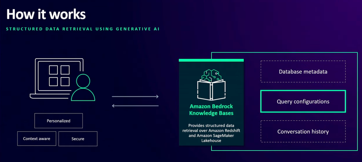
Before we dive into more optimizations options, let’s explore how you can personalize the query engine to generate queries for a specific query engine. In this walkthrough, we use Amazon Redshift. Amazon Bedrock Knowledge Bases analyzes three key components to generate accurate SQL queries:

  • Database metadata
  • Query configurations
  • Historical query and conversation data

The following graphic illustrates this flow.

Amazon Bedrock Knowledge Bases architecture diagram showing structured data retrieval workflow with generative AI

You can configure these settings to enhance query accuracy in two ways:

  • When creating a new Amazon Redshift knowledge base
  • By editing the query engine settings of an existing knowledge base

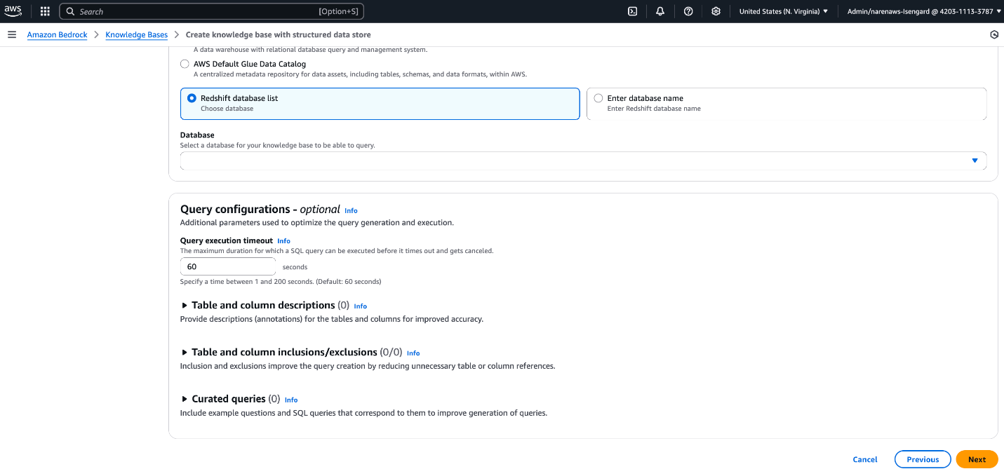
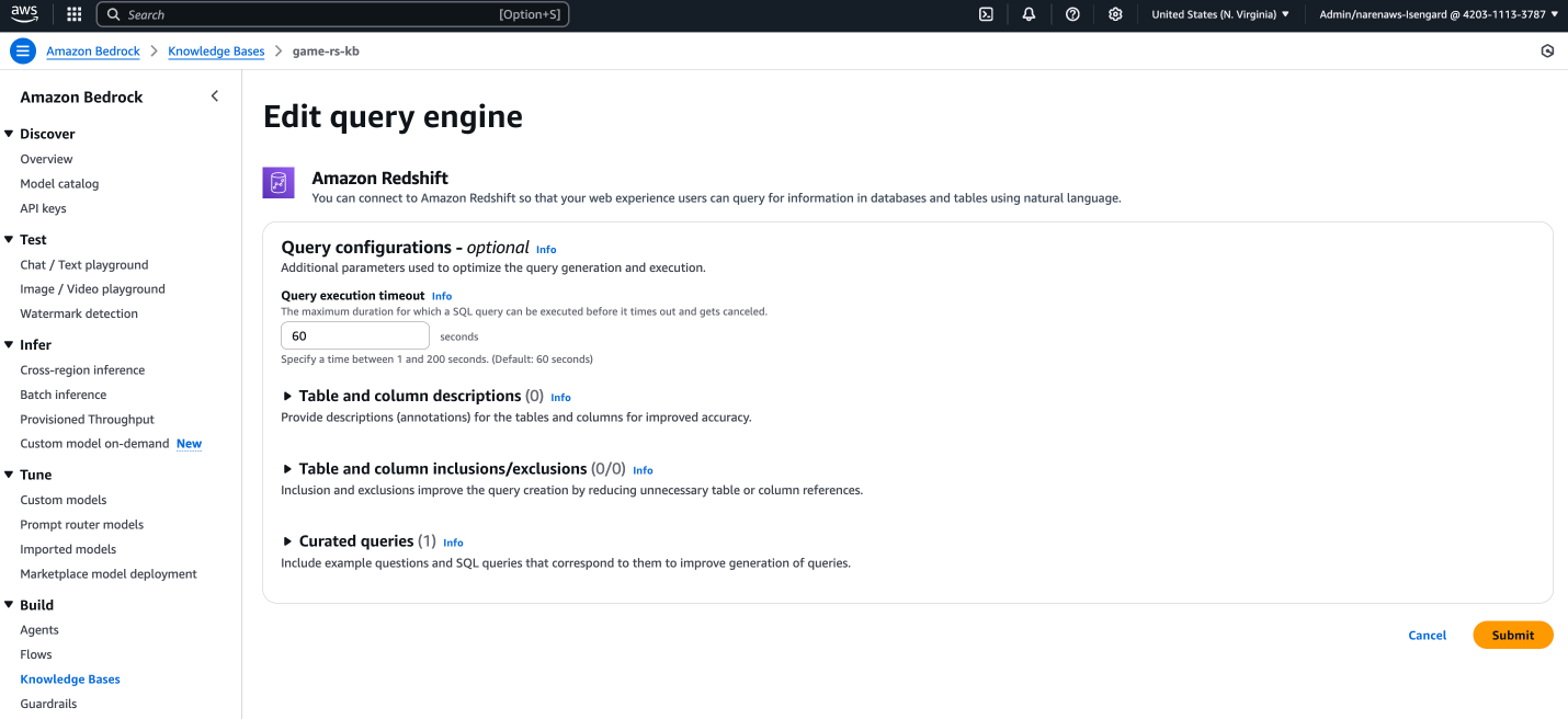
To configure setting when creating new knowledge base, follow steps on Create a knowledge base by connecting to a structured data store and configure below parameters in (Optional) Query configurations section as shown in following screenshot:

  1. Table and column descriptions
  2. Table and column inclusions/exclusions
  3. Curated queries

Amazon Bedrock Knowledge Base creation interface showing Redshift database configuration options

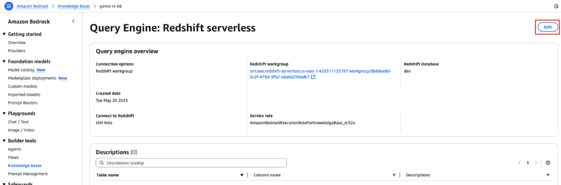
To configure setting when editing the query engine of an existing knowledge base, follow these steps:

  1. On the Amazon Bedrock console in the left navigation pane, choose Knowledge Bases and select your Redshift Knowledge Base.
  2. Choose your query engine and choose Edit,
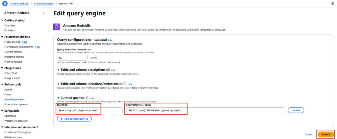
  3. Configure below parameters in (Optional) Query configurations section as shown in following screenshot:
    1. Table and column descriptions
    2. Table and column inclusions/exclusions
    3. Curated queries

Edit query engine configuration page for Amazon Bedrock Knowledge Base with Redshift settings

Let’s explore the available query configuration options in more detail to understand how these help the knowledge base generate a more accurate response.

Table and column descriptions provide essential metadata that helps Amazon Bedrock Knowledge Bases understand your data structure and generate more accurate SQL queries. These descriptions can include table and column purposes, usage guidelines, business context, and data relationships.

Follow these best practices for descriptions:

  • Use clear, specific names instead of abstract identifiers
  • Include business context for technical fields
  • Define relationships between related columns

For example, consider a gaming table with timestamp columns named t1, t2, and t3. Adding these descriptions helps the knowledge base generate appropriate queries. For example, if t1 is play start time, t2 is play end time, and t3 is record creation time, adding these descriptions will indicate to the knowledge base to use t2–t1 for finding the game duration.

Curated queries are a set of predefined question and answer examples. Questions are written as natural language queries (NLQs) and answers are the corresponding SQL query. These examples help the SQL generation process by providing examples of the kinds of queries that should be generated. They serve as reference points to improve the accuracy and relevance of generative SQL outputs. Using this option, you can provide some example queries to the knowledge base for it understand custom vocabulary also. For example, if the country field in the table is populated with a country code, adding an example query will help the knowledge base to convert the country name to a country code before running the query to answer questions on the data of players in a specific country. You can also provide some example complex queries to help the knowledge base to respond to more complex questions. The following is an example query that can be added to the knowledge base:

Select count(*) from players_address where country = ‘USA’;

With table and column inclusion and exclusion, you can specify a set of tables or columns to be included or excluded for SQL generation. This field is crucial if you want to limit the scope of SQL queries to a defined subset of available tables or columns. This option can help optimize the generation process by reducing unnecessary table or column references. You can also use this option to:

  • Exclude redundant tables, for example, those generated by copying the original table to run a complex analysis
  • Exclude tables and columns containing sensitive data

If you specify inclusions, all other tables and columns are ignored. If you specify exclusions, the tables and columns you specify are ignored.

Walkthrough for defining and using curated queries to improve accuracy

To define and use curated queries to improve accuracy, complete the following steps.

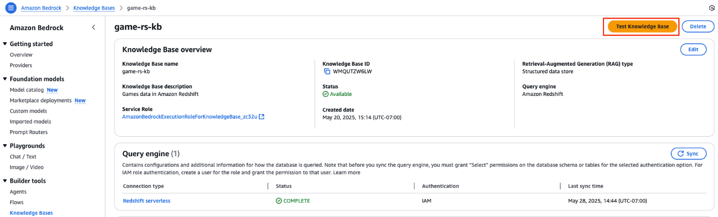
  1. On the AWS Management Console, navigate to Amazon Bedrock and in the left navigation pane, choose Knowledge Bases. Select the knowledge base you created with Amazon Redshift.
  2. Choose Test Knowledge Base, as shown in the following screenshot, to validate the accuracy of the knowledge base response.
    Amazon Bedrock Knowledge Base overview page showing game-rs-kb configuration and status details
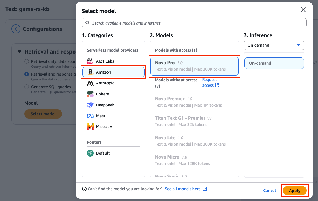
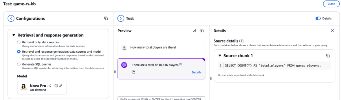
  3. On the Test Knowledge Base screen under Retrieval and response generation, choose Retrieval and response generation: data sources and model.
  4. Choose Select model to pick a large language model (LLM) to convert the SQL query response from the knowledge base to a natural language response.
  5. Choose Nova Pro in the popup and choose Apply, as shown in the following screenshot.
    Model selection dialog showing Amazon Nova Pro and other foundation models for Bedrock Knowledge Base

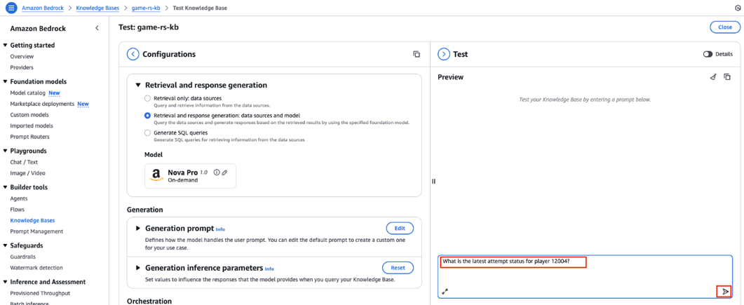
Now you have Amazon Nova Pro connected to your knowledge base to respond to your queries based on the data available in Amazon Redshift. You can ask some questions and verify them with actual data in Amazon Redshift. Follow these steps:

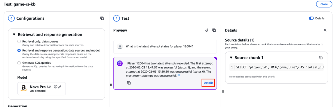
  1. In the Test section on the right, enter the following prompt, then choose the send message icon, as shown in the following screenshot.
    What is the latest attempt status for player 12004?

    Amazon Bedrock Knowledge Base test interface with configuration panel and preview section

  2. Amazon Nova Pro generates a response using the data stored in the Redshift knowledge base.
  3. Choose Details to see the SQL query generated and used by Amazon Nova Pro, as shown in the following screenshot.
    Test results showing AI-generated response with source details for player attempt status query
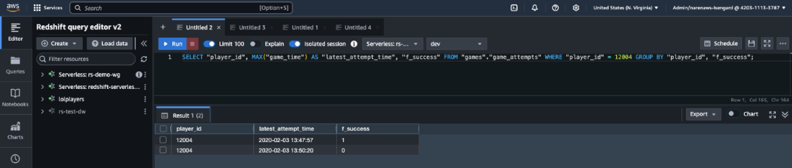
  4. Copy the query and enter it in query editor v2 of the Redshift knowledge base, as shown in the following screenshot.
    AWS Redshift Query Editor showing SQL query execution with player game attempt results
  5. Verify that the response generated by Amazon Nova Pro in natural language matches the data in Amazon Redshift and that the generated SQL query is also accurate.

You can try some more questions to verify the Amazon Nova Pro response, for example:

What is the lost status for player ID 12004?
How many levels did the player 12004 play?
What level did player 12004 play the most?
Show me the summary of all 14 attempts by player 12004 for level 76.

But what if the response generated by the knowledge base isn’t accurate? In those cases, you can add additional context the knowledge base can use to provide more accurate responses. For example, try asking the following question:

How many total players are there?

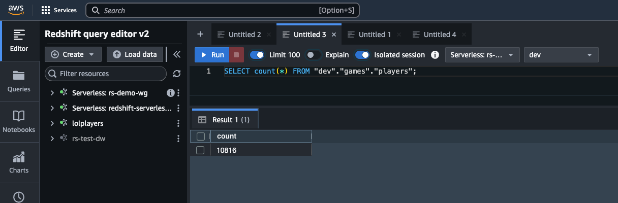
In this case, the response generated by the knowledge base doesn’t match the actual player count in Amazon Redshift. The knowledge base reported about 13,589 players and generated the following query to get the player count:

SELECT COUNT(DISTINCT player_id) AS "Number of Players" FROM games.game_attempts;

The following screenshot shows this question and result.

Test preview showing AI response to player count query with citation

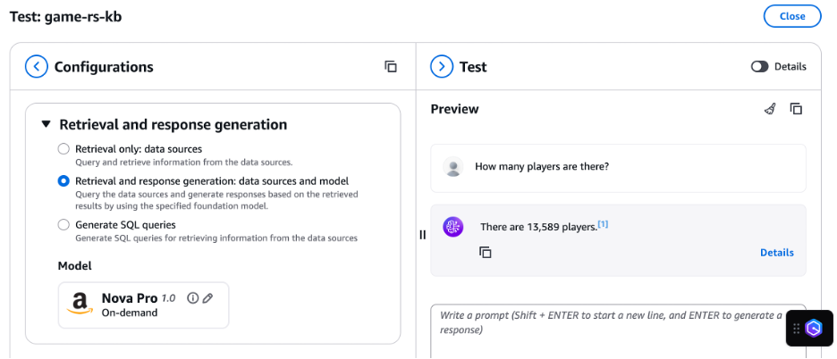
The knowledge base should have used the players table in Amazon Redshift to find the unique players. The correct response is 10,816 players.

AWS Redshift Query Editor showing COUNT query result of 10,816 players

To help the knowledge base, add a curated query for it to use the players table instead of the attempts table to find the total player count. Follow these steps:

  1. On the Amazon Bedrock console in the left navigation pane, choose Knowledge Bases and select your Redshift Knowledge Base.
  2. Choose your query engine and choose Edit, as shown in the following screenshot.
    Amazon Bedrock Query Engine configuration page showing Redshift serverless connection details
  3. Expand the Curated queries section and enter the following:
  4. In the Questions field, enter How many total players are there?.
  5. In the Equivalent SQL query field, enter SELECT count(*) FROM “dev”,“games”,“players”;.
  6. Choose Submit, as shown in the following screenshot.
    Edit query engine page showing curated query example for player count
  7. Navigate back to your knowledge base and query engine. Choose Sync to sync the knowledge base. This starts the metadata ingestion process so that data can be retrieved. The metadata allows Amazon Bedrock Knowledge Bases to translate user prompts into a query for the connected database. Refer to Sync your structured data store with your Amazon Bedrock knowledge base for more details.
  8. Return to Test Knowledge Base with Amazon Nova Pro and repeat the question about how many total players there are, as shown in the following screenshot. Now, the response generated by the knowledge base matches the data in player table in Amazon Redshift, and the query generated by the knowledge base uses the curated query with the player table instead of the attempts table to determine the player count.
    Test results showing total player count query with SQL source details

Cleanup

For the walkthrough section, we used serverless services, and your cost will be based on your usage of these services. If you’re using provisioned Amazon Redshift as a knowledge base, follow these steps to stop incurring charges:

  1. Delete the knowledge base in Amazon Bedrock.
  2. Shut down and delete your Redshift cluster.

Conclusion

In this post, we discussed how you can use Amazon Redshift as a knowledge base to provide additional context to your LLM. We identified best practices and explained how you can improve the accuracy of responses from the knowledge base by following these best practices.


About the authors

Narendra Gupta

Narendra Gupta

Narendra is a Specialist Solutions Architect at AWS, helping customers on their cloud journey with a focus on AWS analytics services. Outside of work, Narendra enjoys learning new technologies, watching movies, and visiting new places.

Satesh Sonti

Satesh Sonti

Satesh is a Principal Analytics Specialist Solutions Architect based out of Atlanta, specializing in building enterprise data platforms, data warehousing, and analytics solutions. He has over 19 years of experience in building data assets and leading complex data platform programs for banking and insurance clients across the globe.

Power up your analytics with Amazon SageMaker Unified Studio integration with Tableau, Power BI, and more

Post Syndicated from Narendra Gupta original https://aws.amazon.com/blogs/big-data/power-up-your-analytics-with-amazon-sagemaker-unified-studio-integration-with-tableau-power-bi-and-more/

Organizations face challenges in accessing and analyzing governed data across multiple sources through their preferred business intelligence (BI) and analytics tools while maintaining security and governance. They need a seamless way to connect their familiar tools (like Tableau, Power BI, Excel) to Amazon SageMaker‘s data assets without compromising data governance and security protocols.

Amazon SageMaker supports authentication through the Amazon Athena JDBC driver, allowing data users to query their subscribed data lake assets via popular BI and analytics tools like Tableau, Power BI, Excel, SQL Workbench, DBeaver, and more. This integration empowers data users to access and analyze governed data within Amazon SageMaker using familiar tools, boosting both productivity and flexibility.

Customers use Amazon SageMaker Unified Studio to streamline data access and governance by enabling data users to locate and subscribe to data from multiple sources within a single project. Amazon SageMaker Unified Studio natively integrates with Amazon-specific options like Amazon AthenaAmazon Redshift, and Amazon SageMaker AI, allowing users to analyze their project governed data. With this launch of JDBC connectivity, Amazon SageMaker Unified Studio expands its support for data users, including analysts and scientists, allowing them to work in their preferred tools, whether it’s SQL Workbench, Domino, or Amazon-native solutions like Amazon Athena, while ensuring secure, governed access within Amazon SageMaker Unified Studio.

Getting Started

To get started, download and install the latest Athena JDBC driver for your tool of choice. After installation, copy the JDBC connection string from the Amazon SageMaker Unified Studio portal into the JDBC connection configuration to establish a connection from your tool. This directs you to authenticate using single sign-on (SSO) with your corporate credentials. After connecting, you can query, visualize, and share data—governed by Amazon SageMaker Unified Studio–within the tools you already know and trust.

In this post, we guide you through connecting various analytics tools to Amazon SageMaker Unified Studio using the Athena JDBC driver, enabling seamless access to your subscribed data within your Amazon SageMaker Unified Studio projects.

Solution overview

To demonstrate these capabilities, consider a use case where your marketing team wants to analyze sales data to understand patterns in sales by stores and sales representatives. To achieve this, your marketing team needs access to sales_performance_by_store, and sales_performance_by_rep data owned by the sales team. The sales team, acting as the data producer, publishes the necessary data assets to Amazon SageMaker Unified Studio, allowing the marketing team, as a consumer, to discover and subscribe to these assets.

After the subscription is approved, the data assets become available within the marketing team’s project environment in Amazon SageMaker Unified Studio. The marketing team can then use their preferred tool to perform data exploration. An example architecture of how this is done using DBeaver is shown in the following image:

SageMaker Unified Studio project architecture diagram showing data collaboration between Sales and Marketing teams with Amazon S3 storage and Athena integration

Prerequisites

To follow along with this post, you need the following prerequisites in place:

  1. AWS account – If you don’t have an active AWS account, see How do I create and activate a new AWS account?.
  2. Amazon SageMaker resources – You need a domain for Amazon SageMaker, and two Amazon SageMaker project.
  3. Publish data assets – As the data producer from the sales team, you can now ingest individual data assets into Amazon SageMaker Unified Studio. For this use case, create a data source and import the technical metadata of two data assets – sales_performance_by_store, and sales_performance_by_rep – from AWS Glue Data Catalog. Ensure the data assets are enriched with business descriptions and published to the catalog.
    Note: Here we are using tables which are in the Glue catalog but with Sagemaker Lakehouse you have the option to bring assets from other sources.
  4. Subscribe data assets – As a data analyst from the marketing team, you can now discover and subscribe to the data assets. The data producer from the retail team reviews and approves your subscription. Upon successful fulfillment, the data assets are added to your SageMaker Unified project.

For detailed instructions for publishing and subscribing, see the Amazon SageMaker Unified Studio User Guide.

The following figure shows the subscribed assets added to the subscribed assets section in your marketing project catalog.

SageMaker Unified Studio Assets page displaying subscribed data assets with accessibility status indicators

In the following sections, we walk you through the steps to configure DBeaver to consume the subscribed assets from Amazon SageMaker Unified Studio.

Configuring DBeaver to access subscribed data assets

In this section, you configure DBeaver to access the subscribed assets from the Marketing project

To configure DBeaver:

  1. Connect with JDBC: In the Amazon SageMaker Unified Studio, (1) open the Marketing project, (2) on the Project overview screen, (3) choose JDBC connection details tab.
    SageMaker Unified Studio Project overview page showing JDBC connection parameters for external application integration
  2. Copy the JDBC connection URL into a text editor. The URL should have the following parameters needed for configuring the database connection in DBeaver – Domain ID, Environment ID, Region, and IDC Issuer URL.
    JDBC connection details configuration panel with IDC authentication parameters and copy functionality
  3. Download and install the latest Athena driver:
    • If DBeaver has the Athena driver pre-installed, it might be the older (v2) version. To ensure compatibility with Amazon SageMaker Unified Studio, you need the latest driver (v3), which includes the necessary authentication features.
    • Download the latest JDBC driver—version 3.x.
    • To install the latest driver:
      • Go to Database and then to Driver Manager in DBeaver.
      • Select the Athena driver and choose Edit.
      • Visit the Libraries tab.
      • Choose Download/Update to fetch the latest driver version.
      • If prompted, select the appropriate version and confirm the download.
  4. In the DBeaver SQL client, create a new database connection and select the Athena driver.
    DBeaver database connection dialog showing Amazon Athena driver selection among available database options
  5. Switch to the Driver Properties tab, enter the values of the following properties that are available in the JDBC connection URL you copied from Amazon SageMaker Unified Studio. If any of these properties are not already available, you can add them and provide their respective values.
    • CredentialsProvider: The credentials provider to authenticate requests to AWS
    • DataZoneDomainId: The ID of your Amazon DataZone domain
    • DataZoneDomainRegion: The AWS Region where your domain is hosted
    • DataZoneEnvironmentId: The ID of your DefaultDataLake environment
    • IdentityCenterIssuerUrl: The issuer URL used by AWS Identity and Access Management (IAM) Identity Center for token issuance
    • OutputLocation: Amazon S3 path for storing query results
    • Region: The Region where the environment is created
    • Workgroup: Amazon Athena workgroup of the environment
    • ListenPort: Pick any four digits port number. This is the port number that listens for the IAM Identity Center response

    DBeaver connection configuration dialog for Amazon Athena with driver properties and authentication settings

  6. Choose Test Connection….
  7. You are redirected to the IAM Identity Center sign-in portal. Sign in with Marketing user credentials. If you’re already signed in through single sign-on (SSO), this step can be skipped.
    AWS authentication sign-in page with username input field
  8. After you sign in, if you are prompted to authorize the DataZoneAuthPlugin. Choose Allow access to authorize access to Amazon DataZone from DBeaver.
    AWS DataZone authorization dialog requesting user permission for application access
  9. After sign in completes, you see the following message. You can close the window and go to the DBeaver.
    Amazon DataZone session completion confirmation message
  10. After the connection is established, the following success message appears.
    DBeaver connection test dialog showing successful Amazon Athena connection with performance metrics
  11. You can now view and query all subscribed assets directly within DBeaver.
    DBeaver SQL query interface displaying sales performance data from Amazon Athena database

These steps might also apply to other analytics tools and clients that support JDBC connections. If you’re using a different tool, you might need to adapt these instructions accordingly to ensure proper configuration and access to Amazon SageMaker Unified Studio data assets.

Integration with other applications

You can use similar steps for other BI and analytics tools that support standard database connections.

Connect to Tableau Desktop

Use the Athena JDBC driver to connect Tableau to Amazon SageMaker Unified Studio and visualize your subscribed data.To connect to Tableau Desktop:

  1. Make sure that you’re using the latest Athena JDBC 3.x driver.
  2. Copy the JDBC driver file and place it in the appropriate folders for your operating system
    • For Mac OS: ~/Library/Tableau/Drivers
    • For Windows: C:\Program Files\Tableau\Drivers
  3. Open Tableau Desktop. From the To a Server connection menu, select Other Databases (JDBC) to connect to Amazon SageMaker Unified Studio.
    Tableau start page showing connection options with Other Databases JDBC option highlighted
  4. Paste the JDBC connection URL you copied from the SageMaker Unified Studio portal into the URL. Leave other fields such as DialectUsername, and Password blank and choose Sign in.
    If you get a port is occupied error – add “;ListenPort=8055” to the URL to change the port. You can use any port number.

    Tableau Other Databases JDBC connection dialog with PostgreSQL dialect configuration

  5. This redirects you to authenticate with IAM Identity Center. Enter the credentials of the Identity Center user that you used to sign in to the SageMaker Unified Studio portal. Authorize the DataZoneAuthPlugin to access Amazon DataZone from Tableau. Once the connection is established with the success message, you can view your project’s subscribed data directly within Tableau and build dashboards.
    Data analytics interface showing sales_performance_by_store table with 283 rows and 15 fields

Connect to Microsoft Power BI

Now, we look at connecting Amazon SageMaker Unified Studio with Microsoft Power BI on Windows.While Amazon Athena provides a native ODBC driver for connecting to ODBC-compatible tools like Microsoft Power BI, it currently doesn’t support Amazon SageMaker Unified Studio authentication. Therefore, in this post, we use an ODBC-JDBC bridge to connect Amazon SageMaker Unified Studio with Microsoft Power BI using the Athena JDBC driver, which supports SageMaker Unified Studio authentication.

In this post, we’re using the ZappySys driver as the ODBC-JDBC bridge. This is a third-party solution that requires a separate licensing fee, which isn’t included in the AWS solution. You can choose to use any other solution for ODBC-JDBC bridge.To connect to Power BI:

  1. Make sure that you have administrator privileges to run the ODBC Data Source Administrator.
  2. From the Windows Start menu, run the ODBC Data Source Administrator (the 64-bit version) using run as Administrator.
  3. Create a New Data Source with the ZappySys JDBC Bridge Driver. You are prompted to enter your connection details.
    Windows ODBC Data Source Administrator dialog showing ZappySys JDBC Bridge Driver selection
  4. Paste the JDBC URL you copied from the SageMaker Unified Studio portal in the Connection String, along with the driver class and JDBC driver file. Make sure that you’re using the latest Athena JDBC 3.x driver.
  5. Choose Test Connection. A new dialog window pops up after the connection is successful.
    Test Connection using ZappySys JDBC Bridge Driver
  6. This redirects you to authenticate with IAM Identity Center. Enter the credentials of the Identity Center user that you used to sign in to the SageMaker Unified Studio portal. Authorize the DataZoneAuthPlugin.
  7. Choose Preview tab on ZappySys JDBC Bridge Driver window and choose one of the subscribed tables to access data.
    ZappySys JDBC Bridge Driver configuration interface showing SQL query preview with sales performance results
  8. After configuring the data source, launch Power BI. Create a blank report or use an existing report to integrate the new visuals. Choose Get Data and select the name of the data source you created. This opens a new browser window to authenticate your credentials. Allow access to authorize the DataZone Auth plugin. After authorization is complete, you can build your reports in Microsoft Power BI with the subscribed data assets.
    Database connection profile selection dialog with PostgreSQL group highlighted

Connect to SQL Workbench

Discover how SQL Workbench can connect to Amazon SageMaker Unified Studio for users who prefer a SQL interface to query data lake tables and views subscribed through projects in Amazon SageMaker Unified Studio.

To connect to SQL Workbench:

  1. Make sure that you’re using the latest Athena JDBC 3.x driver.
  2. Open SQL Workbench/J and choose Manage Drivers.
    Database driver management interface showing SMUSAthenajDBC driver configuration details
  3. Select the option to add a new driver. Enter a name for it, such as SMUSAthenaJDBC, and import the driver you downloaded in the previous steps.
    Database driver management dialog showing SMUSAthenaJDBC driver configuration with library path and class name
  4. Create a new connection profile and enter a name it, such as smus-profile. In the Driver dropdown, select the driver you configured. For the URL, enter the string jdbc:athena://region=us-east-1; (In the example, the Virginia Region is being used). Choose Extended Properties.
    PostgreSQL connection profile configuration dialog with Amazon Athena JDBC driver settings and authentication options
  5. Under Extended Properties, add the following parameters that you copied from the SageMaker Unified Studio portal. You can also include these parameters in the JDBC (URL) connection string. Choose OK.
    • Workgroup
    • OutputLocation
    • DataZoneDomainId
    • IdentityCenterIssuerURL
    • CredentialsProvider
    • DatazoneEnvironmentId
    • DataZoneDomainRegain

    Alos add “ListenPort” with any port number.

    Extended properties configuration dialog showing AWS DataZone connection parameters including domain ID, environment ID, and listen port 8067

  6. This redirects you to authenticate with IAM Identity Center. Enter the credentials of the Identity Center user that you used to sign in to the SageMaker Unified Studio portal. Authorize the DataZoneAuthPlugin.
  7. After successful connection, in SQL Workbench/J, under Database Explorer, select the database from the marketing project of SageMaker unified studio. Choose a subscribed table. Select the Data tab to see the data in the table.
    SQL Workbench showing sales performance data query results from AWS Athena database with 283 customer transaction records

Cleanup

To ensure no additional charges are incurred after testing, be sure to delete the Amazon SageMaker Unified Studio domain. See Delete domains for instructions.

Conclusion

Amazon SageMaker Unified Studio continues to expand its offerings, providing you with more flexibility to access, analyze, and visualize your subscribed data. With support for the Athena JDBC driver, you can now use a wide range of popular BI and analytics tools, making data accessed through Amazon SageMaker Unified Studio more accessible than ever before. Whether you’re using Tableau, Power BI, or other familiar tools, the integration with Amazon SageMaker Unified Studio ensures that your data remains secure and accessible to authorized users.

The feature is supported in all AWS commercial Regions where Amazon SageMaker Unified Studio is currently available. Get started with our technical documentation.


About the authors

Narendra Gupta

Narendra Gupta

Narendra is a Specialist Solutions Architect at AWS, helping customers on their cloud journey with a focus on AWS analytics services. Outside of work, Narendra enjoys learning new technologies, watching movies, and visiting new places.

Durga Mishra

Durga Mishra

Durga is a solutions architect at AWS. Outside of work, Durga enjoys spending time with family and loves to hike on Appalachian trails and spend time in nature.

Ramesh Singh

Ramesh Singh

Ramesh is a Senior Product Manager Technical (External Services) at AWS in Seattle, Washington, currently with the Amazon SageMaker team. He is passionate about building high-performance ML/AI and analytics products that help enterprise customers achieve their critical goals using cutting-edge technology.

Nishchai JM

Nishchai JM

Nishchai is an Analytics Specialist Solutions Architect at Amazon Web services. He specializes in building Big-data applications and help customer to modernize their applications on Cloud. He thinks Data is new oil and spends most of his time in deriving insights out of the Data.

Identify source schema changes using AWS Glue

Post Syndicated from Narendra Gupta original https://aws.amazon.com/blogs/big-data/identify-source-schema-changes-using-aws-glue/

In today’s world, organizations are collecting an unprecedented amount of data from all kinds of different data sources, such as transactional data stores, clickstreams, log data, IoT data, and more. This data is often in different formats, such as structured data or unstructured data, and is usually referred to as the three Vs of big data (volume, velocity, and variety). To extract information from the data, it’s usually stored in a data lake built on Amazon Simple Storage Service (S3). The data lake provides an important characteristic called schema on read, which allows you to bring data in the data lake without worrying about the schema or changes in the schema on the data source. This enables faster ingestion of data or building data pipelines.

However, you may be reading and consuming this data for other use cases, such as pointing to applications, building business intelligence (BI) dashboards in services like Amazon QuickSight, or doing data discovery using a serverless query engine like Amazon Athena. Additionally, you may have built an extract, transform, and load (ETL) data pipeline to populate your data store like a relational database, non-relational database, or data warehouse for further operational and analytical needs. In these cases, you need to define the schema upfront or even keep an account of the changes in the schema, such as adding new columns, deleting existing columns, changing the data type of existing columns, or renaming existing columns, to avoid any failures in your application or issues with your dashboard or reporting.

In many use cases, we have found that the data teams responsible for building the data pipeline don’t have any control of the source schema, and they need to build a solution to identify changes in the source schema in order to be able to build the process or automation around it. This might include sending notifications of changes to the teams dependent on the source schema, building an auditing solution to log all the schema changes, or building an automation or change request process to propagate the change in the source schema to downstream applications such as an ETL tool or BI dashboard. Sometimes, to control the number of schema versions, you may want to delete the older version of the schema when there are no changes detected between it and the newer schema.

For example, assume you’re receiving claim files from different external partners in the form of flat files, and you’ve built a solution to process claims based on these files. However, because these files were sent by external partners, you don’t have much control over the schema and data format. For example, columns such as customer_id and claim_id were changed to customerid and claimid by one partner, and another partner added new columns such as customer_age and earning and kept the rest of the columns the same. You need to identify such changes in advance so you can edit the ETL job to accommodate the changes, such as changing the column name or adding the new columns to process the claims.

In this solution, we showcase a mechanism that simplifies the capture of the schema changes in your data source using an AWS Glue crawler.

Solution overview

An AWS Glue data crawler is built to sync metadata based on existing data. After we identify the changes, we use Amazon CloudWatch to log the changes and Amazon Simple Notification Service (Amazon SNS) to notify the changes to the application team over email. You can expand this solution to solve for other use cases such as building an automation to propagate the changes to downstream applications or pipelines, which is out of scope for this post, to avoid any failures in downstream applications because of schema changes. We also show a way to delete older versions of the schema if there are no changes between the compared schema versions.

If you want to capture the change in an event-driven manner, you can do so by using Amazon EventBridge. However, if you want to capture the schema changes on multiple tables at the same time, based on a specific schedule, you can use the solution in this post.

In our scenario, we have two files, each with different schemas, simulating data that has undergone a schema change. We use an AWS Glue crawler to extract the metadata from data in an S3 bucket. Then we use an AWS Glue ETL job to extract the changes in the schema to the AWS Glue Data Catalog.

AWS Glue provides a serverless environment to extract, transform, and load a large number of datasets from several sources for analytic purposes. The Data Catalog is a feature within AWS Glue that lets you create a centralized data catalog of metadata by storing and annotating data from different data stores. Examples include object stores like Amazon S3, relational databases like Amazon Aurora PostgreSQL-Compatible Edition, and data warehouses like Amazon Redshift. You can then use that metadata to query and transform the underlying data. You use a crawler to populate the Data Catalog with tables. It can automatically discover new data, extract schema definitions, detect schema changes, and version tables. It can also detect Hive-style partitions on Amazon S3 (for example year=YYYY, month=MM, day=DD).

Amazon S3 serves as the storage for our data lake. Amazon S3 is an object storage service that offers industry-leading scalability, data availability, security, and performance.

The following diagram illustrates the architecture for this solution.

The workflow includes the following steps:

  1. Copy the first data file to the data folder of the S3 bucket and run the AWS Glue crawler to create a new table in the Data Catalog.
  2. Move the existing file from the data folder to the archived folder.
  3. Copy the second data file with the updated schema to the data folder, then rerun the crawler to create new version of table schema.
  4. Run the AWS Glue ETL job to check if there is a new version of the table schema.
  5. The AWS Glue job lists the changes in the schema with the previous version of the schema in CloudWatch Logs. If there are no changes in the schema and the flag to delete older versions is set to true, the job also deletes the older schema versions.
  6. The AWS Glue job notifies all changes in the schema to the application team over email using Amazon SNS.

To build the solution, complete the following steps:

  1. Create an S3 bucket with the data and archived folders to store the new and processed data files.
  2. Create an AWS Glue database and an AWS Glue crawler that crawls the data file in the data folder to create an AWS Glue table in the database.
  3. Create an SNS topic and add an email subscription.
  4. Create an AWS Glue ETL job to compare the two versions of the table schema, list the changes in the schema with the older version of schema, and delete older versions of schema if the flag to delete older versions is set to true. The job also publishes an event in Amazon SNS to notify the changes in the schema to the data teams.

For the purpose of this post, we manually perform the steps to move the data files from the data folder to the archive folder, triggering the crawler and ETL job. Depending on your application needs, you can automate and orchestrate this process through AWS Glue workflows.

Let’s set up the infrastructure required to go through the solution to compare an AWS Glue table version to a version updated with recent schema changes.

Create an S3 bucket and folders

To create an S3 bucket with the data and archived folders to store the new and processed data files, complete the following steps:

  1. On the Amazon S3 console, choose Buckets in the navigation pane.
  2. Choose Create bucket.
  3. For Bucket name, enter a DNS-compliant unique name (for example, aws-blog-sscp-ng-202202).
  4. For Region, choose the Region where you want the bucket to reside.
  5. Keep all other settings as default and choose Create bucket.
  6. On the Buckets page, choose the newly created bucket.
  7. Choose Create folder.
  8. For Folder name, enter data.
  9. Leave server-side encryption at its default (disabled).
  10. Choose Create folder.
  11. Repeat these steps to create the archived folder in the same bucket.

Create an AWS Glue database and crawler

Now we create an AWS Glue database and crawler that crawls the data file in the data bucket to create an AWS Glue table in the new database.

  1. On the AWS Glue console, choose Databases in the navigation pane.
  2. Choose Add database.
  3. Enter a name (for example, sscp-database) and description.
  4. Choose Create.
  5. Choose Crawlers in the navigation pane.
  6. Choose Add crawler.
  7. For Crawler name, enter a name (glue-crawler-sscp-sales-data).
  8. Choose Next.
  9. For the crawler source type¸ choose Data stores.
  10. To repeat crawls of the data stores, choose Crawl all folders.
  11. Choose Next.
  12. For Choose a data store, choose S3.
  13. For Include path, choose the S3 bucket and folder you created (s3://aws-blog-sscp-ng-202202/data).
  14. Choose Next.
  15. On the Add another data store page, choose No, then choose Next.
  16. Choose Create an IAM role and enter a name for the role (for example, sscp-blog).
  17. Choose Next.
  18. Choose Run on Demand, then choose Next.
  19. For Database, choose your AWS Glue database (sscp-database).
  20. For Prefix added to tables, enter a prefix (for example, sscp_sales_).
  21. Expand the Configuration options section and choose Update the table definition in the data catalog.
  22. Leave all other settings as default and choose Next.
  23. Choose Finish to create the crawler.

Create an SNS topic

To create an SNS topic and add an email subscription, complete the following steps:

  1. On the Amazon SNS console, choose Topics in the navigation pane.
  2. Choose Create topic.
  3. For Type, choose Standard.
  4. Enter a name for the topic (for example, NotifySchemaChanges).
  5. Leave all other settings as default and choose Create topic.
  6. In the navigation pane, choose Subscriptions.
  7. Choose Create subscription.
  8. For Topic ARN, choose the ARN of the created SNS topic.
  9. For Protocol, choose Email.
  10. For Endpoint, enter the email address to receive notifications.
  11. Leave all other defaults and choose Create subscription.You should receive an email to confirm the subscription.
  12. Choose the link in the email to confirm.
  13. Add the following permission policy to the AWS Glue service role created earlier as part of the crawler creation (AWSGlueServiceRole-sscp-blog) to allow publishing to the SNS topic. Make sure to change <$SNSTopicARN> in the policy with the actual ARN of the SNS topic.
{
    "Version": "2012-10-17",
    "Statement": [
        {
            "Sid": "AllowEventPublishing",
            "Effect": "Allow",
            "Action": "sns:Publish",
            "Resource": "<$SNSTopicARN>"
        }
    ]
}

Create an AWS Glue ETL job

Now you create an AWS Glue ETL job to compare two schema versions of a table and list the changes in schemas. If there are no changes in the schema and the flag to delete older versions is set to true, the job also deletes any older versions. If there are changes in schema, the job lists changes in the CloudWatch logs and publishes an event in Amazon SNS to notify changes to the data team.

  1. On the AWS Glue console, choose AWS Glue Studio.
  2. Choose Create and manage jobs.
  3. Choose the Python Shell script editor.
  4. Choose Create to create a Python Shell job.
  5. Enter the following code in the script editor field:
    import boto3
    import pandas as pd
    
    # Input Paramaters:  
    # catalog_id - Your AWS Glue Catalg Id - it is same as your AWS account ID
    # db_name - name of your AWS Glue Database in your Glue Data catalog_id
    # table_name - name of the table in your AWS Glue Database that you would like to check of change in schema
    # topic_arn - ARN of the SNS topic to publish the changes in table schema
    # versions_to_compare - Two versions that customer would want to compare. 0 is the lastes version and 1 in the version prior to the latest version
    # delete_old_versions - If True and there are no changes in the versions compared, job would delete all old versions except for the latest "number_of_versions_to_retain" versions 
    # number_of_versions_to_retain - if delete_old_versions is True and there are no changes in the versions compared, the job would delete all old versions except for the latest "number_of_versions_to_retain" versions
    
    catalog_id = '<$catalog_id>'
    db_name='<$db_name>'
    table_name='<$table_name>'
    topic_arn='<$sns_topic_ARN>'
    versions_to_compare=[0,1]
    delete_old_versions = False
    number_of_versions_to_retain = 2
    
    columns_modified = []
    
    # Function to compare the name and type of columns in new column list with old column list to 
    # find any newly added column and the columns with changed data type
    def findAddedUpdated(new_cols_df, old_cols_df, old_col_name_list):
        for index, row in new_cols_df.iterrows():
            new_col_name = new_cols_df.iloc[index]['Name']
            new_col_type = new_cols_df.iloc[index]['Type']
    
            # Check if a column with same name exist in old table but the data type has chaged
            if new_col_name in old_col_name_list:
                old_col_idx = old_cols_df.index[old_cols_df['Name']==new_col_name][0]
                old_col_type = old_cols_df.iloc[old_col_idx]['Type']
    
                if old_col_type != new_col_type:
                    columns_modified.append(f"Data type changed for '{new_col_name}' from '{old_col_type}' to '{new_col_type}'")
            # If a column is only in new column list, it a newly added column
            else:
                columns_modified.append(f"Added new column '{new_col_name}' with data type as '{new_col_type}'")
    
    # Function to iterate through the list of old columns and check if any column doesn't exist in new columns list to find out dropped columns
    def findDropped(old_cols_df, new_col_name_list):
        for index, row in old_cols_df.iterrows():
            old_col_name = old_cols_df.iloc[index]['Name']
            old_col_type = old_cols_df.iloc[index]['Type']
    
            #check if column doesn't exist in new column list  
            if old_col_name not in new_col_name_list:
                columns_modified.append(f"Dropped old column '{old_col_name}' with data type as '{old_col_type}'")
    
    # Function to publish changes in schema to a SNS topic that can be subscribed to receive email notifications when changes are detected
    def notifyChanges(message_to_send):
        sns = boto3.client('sns')
        # Publish a simple message to the specified SNS topic
        response = sns.publish(
            TopicArn=topic_arn,   
            Message=message_to_send,  
            Subject="DWH Notification: Changes in table schema"
        )
        
    # Function to convert version_id to int to use for sorting the versions
    def version_id(json):
        try:
            return int(json['VersionId'])
        except KeyError:
            return 0
    
    # Function to delete the table versions
    def delele_versions(glue_client, versions_list, number_of_versions_to_retain):
        print("deleting old versions...")
        if len(versions_list) > number_of_versions_to_retain:
            version_id_list = []
            for table_version in versions_list:
                version_id_list.append(int(table_version['VersionId']))
            # Sort the versions in descending order
            version_id_list.sort(reverse=True)
            versions_str_list = [str(x) for x in version_id_list]
            versions_to_delete = versions_str_list[number_of_versions_to_retain:]
            
            del_response = glue_client.batch_delete_table_version(
                DatabaseName=db_name,
                TableName=table_name,
                VersionIds=versions_to_delete
            )
            return del_response
    
    # Calling glue API to get the list of table versions. The solution assums that number of version in the table are less than 100. If you have more than 100 versions, you should use pagination and loop through each page.  
    glue = boto3.client('glue')
    response = glue.get_table_versions(
        CatalogId=catalog_id,
        DatabaseName=db_name,
        TableName=table_name,
        MaxResults=100
    )
    table_versions = response['TableVersions']
    table_versions.sort(key=version_id, reverse=True)
    
    version_count = len(table_versions)
    print(version_count)
    
    # checking if the version of table to compare exists. You would need pass the numbers of versions to compare to the job. 
    if version_count > max(versions_to_compare):
    
        new_columns = table_versions[versions_to_compare[0]]['Table']['StorageDescriptor']['Columns']
        new_cols_df = pd.DataFrame(new_columns)
    
        old_columns = table_versions[versions_to_compare[1]]['Table']['StorageDescriptor']['Columns']
        old_cols_df = pd.DataFrame(old_columns)
    
        new_col_name_list =  new_cols_df['Name'].tolist()
        old_col_name_list =  old_cols_df['Name'].tolist()
        findAddedUpdated(new_cols_df, old_cols_df, old_col_name_list)
        findDropped(old_cols_df, new_col_name_list)
        if len(columns_modified) > 0: 
            email_msg = f"Following changes are identified in '{table_name}' table of '{db_name}' database of your Datawarehouse. Please review.\n\n"
            print("Job completed! -- below is list of changes.")
            for column_modified in columns_modified:
                email_msg += f"\t{column_modified}\n"
    
            print(email_msg)
            notifyChanges(email_msg)
        else:
            if delete_old_versions:
                delele_versions(glue, table_versions,number_of_versions_to_retain)
            print("Job completed! -- There are no changes in table schema.")
    else:
        print("Job completed! -- Selected table doesn't have the number of versions selected to compare. Please verify the list passed in 'versions_to_compare'")

  6. Enter a name for the job (for example, find-change-job-sscp).
  7. For IAM Role, choose the AWS Glue service role (AWSGlueServiceRole-sscp-blog).
  8. Leave all other defaults and choose Save.

Test the solution

We’ve configured the infrastructure to run the solution. Let’s now see it in action. First we upload the first data file and run our crawler to create a new table in the Data Catalog.

  1. Create a CSV file called salesdata01.csv with the following contents:
    ordertime,region,rep,item,units,unitcost
    2022-01-06,US-West,Jones,Pencil,95,1.99
    2022-01-06,US-Central,Kivell,Binder,50,19.99
    2022-01-07,US-Central,Jardine,Pencil,36,4.99
    2022-01-07,US-Central,Gill,Pen,27,19.99
    2022-01-08,US-East,Sorvino,Pencil,56,2.99
    2022-01-08,US-West,Jones,Binder,60,4.99
    2022-01-09,US-Central,Andrews,Pencil,75,1.99
    2022-01-10,US-Central,Jardine,Pencil,90,4.99
    2022-01-11,US-East,Thompson,Pencil,32,1.99
    2022-01-20,US-West,Jones,Binder,60,8.99

  2. On the Amazon S3 console, navigate to the data folder and upload the CSV file.
  3. On the AWS Glue console, choose Crawlers in the navigation pane.
  4. Select your crawler and choose Run crawler.The crawler takes a few minutes to complete. It adds a table (sscp_sales_data) in the AWS Glue database (sscp-database).
  5. Verify the created table by choosing Tables in the navigation pane.Now we move the existing file in the data folder to the archived folder.
  6. On the Amazon S3 console, navigate to the data folder.
  7. Select the file you uploaded (salesdata01.csv) and on the Actions menu, choose Move.
  8. Move the file to the archived folder.Now we copy the second data file with the updated schema to the data folder and rerun the crawler.
  9. Create a CSV file called salesdata02.csv with the following code. It contains the following changes from the previous version:
    1. The data in the region column is changed from region names to some codes (for example, the data type is changed from string to BIGINT).
    2. The rep column is dropped.
    3. The new column total is added.
      ordertime,region,item,units,unitcost,total
      2022-02-01,01,Pencil,35,4.99,174.65
      2022-02-01,03,Desk,2,125,250
      2022-02-02,01,Pen Set,16,15.99,255.84
      2022-02-02,03,Binder,28,8.99,251.72
      2022-02-03,01,Pen,64,8.99,575.36
      2022-02-03,01,Pen,15,19.99,299.85
      2022-02-06,03,Pen Set,96,4.99,479.04
      2022-02-10,03,Pencil,67,1.29,86.43
      2022-02-11,01,Pen Set,74,15.99,183.26
      2022-02-11,03,Binder,46,8.99,413.54

  10. On the Amazon S3 bucket, upload the file to the data folder.
  11. On the AWS Glue console, choose Crawlers in the navigation pane.
  12. Select your crawler and choose Run crawler.The crawler takes approximately 2 minutes to complete. It updates the schema of the previously created table (sscp_sales_data).
  13. Verify the new version of the table is created on the Tables page.Now we run the AWS Glue ETL job to check if there is a new version of the table schema and list the changes in the schema with the previous version of the schema in CloudWatch Logs.
  14. On the AWS Glue console, choose Jobs in the navigation pane.
  15. Select your job (find-change-job-sscp) and on the Actions menu, choose Edit script.
  16. Change the following input parameters for the job in the script to match with your configuration:
  17. Choose Save.
  18. Close the script editor.
  19. Select the job again and on the Actions menu, choose Run job.
  20. Leave all default parameters and choose Run job.
  21. To monitor the job status, choose the job and review the History tab.
  22. When the job is complete, choose the Output link to open the CloudWatch logs for the job.

The log should show the changes identified by the AWS Glue job.

You should also receive an email with details on the changes in the schema. The following is an example of an email received.

We can now review the changes identified by the AWS Glue ETL job and make changes in the downstream data store accordingly before running the job to propagate the data from the S3 bucket to downstream applications. For example, if you have an Amazon Redshift table, after the job lists all the schema changes, you need to connect to the Amazon Redshift database and make these schema changes. Follow the change request process set by your organization before making schema changes in your production system.

The following table has a list of mappings for Apache Hive and Amazon Redshift data types. You can find similar mappings for other data stores and update your downstream data store.

The provided Python code takes care of the logic to compare the schema changes. The script takes in the parameters of the AWS Glue Data Catalog ID, AWS Glue database name, and AWS Glue table name.

Hive Data Types Description Amazon Redshift Data Types Description
TINYINT 1 byte integer . .
SMALLINT Signed two-byte integer SMALLINT Signed two-byte integer
INT Signed four-byte integer INT Signed four-byte integer
BIGINT Signed eight-byte integer BIGINT Signed eight-byte integer
DECIMAL . . .
DOUBLE . . .
STRING . VARCHAR, CHAR .
VARCHAR 1 to 65355, available starting with Hive 0.12.0 VARCHAR .
CHAR 255 length, available starting with Hive 0.13.0 CHAR .
DATE year/month/day DATE year/month/day
TIMESTAMP No timezone TIME Time without time zone
. . TIMETZ Time with time zone
ARRAY/STRUCTS . SUPER .
BOOLEAN . BOOLEAN .
BINARY . VARBYTE Variable-length binary value

Clean up

When you’re done exploring the solution, clean up the resources you created as part of this walkthrough:

  • AWS Glue ETL job (find-change-job-sscp)
  • AWS Glue crawler (glue-crawler-sscp-sales-data)
  • AWS Glue table (sscp_sales_data)
  • AWS Glue database (sscp-database)
  • IAM role for the crawler and ETL job (AWSGlueServiceRole-sscp-blog)
  • S3 bucket (aws-blog-sscp-ng-202202) with all the files in the data and archived folders
  • SNS topic and subscription (NotifySchemaChanges)

Conclusion

In this post, we showed you how to use AWS services together to detect schema changes in your source data, which you can then use to change your downstream data stores and run ETL jobs to avoid any failures in your data pipeline. We used AWS Glue to understand and catalog the source data schema, AWS Glue APIs to identify schema changes, and Amazon SNS to notify the team about the changes. We also showed you how to delete the older versions of your source data schema using AWS Glue APIs. We used Amazon S3 as our data lake storage tier.

Here you can learn more about AWS Glue.


About the authors

Narendra Gupta is a Specialist Solutions Architect at AWS, helping customers on their cloud journey with a focus on AWS analytics services. Outside of work, Narendra enjoys learning new technologies, watching movies, and visiting new places.

Navnit Shukla is AWS Specialist Solutions Architect in Analytics. He is passionate about helping customers uncover insights from their data. He has been building solutions to help organizations make data-driven decisions.