Post Syndicated from Pathik Shah original https://aws.amazon.com/blogs/big-data/transform-your-data-to-amazon-s3-tables-with-amazon-athena/
Organizations today manage vast amounts of data, with much of it stored based on initial use cases and business needs. As requirements for this data evolve—whether for real-time reporting, advanced machine learning (ML), or cross-team data sharing—the original storage formats and structures often become a bottleneck. When this happens, data teams frequently find that datasets that worked well for their original purpose now require complex transformations; custom extract, transform, and load (ETL) pipelines; and extensive redesign to unblock new analytical workflows. This creates a significant barrier between valuable data and actionable insights.
Amazon Athena offers a solution through its serverless, SQL-based approach to data transformation. With the CREATE TABLE AS SELECT (CTAS) functionality in Athena, you can transform existing data and create new tables in the process, using standard SQL statements to help reduce the need for custom ETL pipeline development.
This CTAS experience now supports Amazon S3 Tables, which provide built-in optimization, Apache Iceberg support, automatic table maintenance, and ACID transaction capabilities. This combination can help organizations modernize their data infrastructure, achieve improved performance, and reduce operational overhead.
You can use this approach to transform data from commonly used tabular formats, including CSV, TSV, JSON, Avro, Parquet, and ORC. The resulting tables are immediately accessible for querying across Athena, Amazon Redshift, Amazon EMR, and supported third-party applications, including Apache Spark, Trino, DuckDB, and PyIceberg.
This post demonstrates how Athena CTAS simplifies the data transformation process through a practical example: migrating an existing Parquet dataset into S3 Tables.
Solution overview
Consider a global apparel ecommerce retailer processing thousands of daily customer reviews across marketplaces. Their dataset, currently stored in Parquet format in Amazon Simple Storage Service (Amazon S3), requires updates whenever customers modify ratings and review content. The business needs a solution that supports ACID transactions—the ability to atomically insert, update, and delete records while maintaining data consistency—because review data changes frequently as customers edit their feedback.
Additionally, the data team faces operational challenges: manual table maintenance tasks like compaction and metadata management, no built-in support for time travel queries to analyze historical changes, and the need for custom processes to handle concurrent data modifications safely.
These requirements point to a need for an analytics-friendly solution that can handle transactional workloads while providing automated table maintenance, reducing the operational overhead that currently burdens their analysts and engineers.
S3 Tables and Athena provide an ideal solution for these requirements. S3 Tables provide storage optimized for analytics workloads, offering Iceberg support with automatic table maintenance and continuous optimization. Athena is a serverless, interactive query service you can use to analyze data using standard SQL without managing infrastructure. When combined, S3 Tables handle the storage optimization and maintenance automatically, and Athena provides the SQL interface for data transformation and querying. This can help reduce the operational overhead of manual table maintenance while providing efficient data management and optimal performance across supported data processing and query engines.
In the following sections, we show how to use the CTAS functionality in Athena to transform the Parquet-formatted review data into S3 Tables with a single SQL statement. We then demonstrate how to manage dynamic data using INSERT, UPDATE, and DELETE operations, showcasing the ACID transaction capabilities and metadata query features in S3 Tables.
Prerequisites
In this walkthrough, we will be working with synthetic customer review data that we’ve made publicly available at s3://aws-bigdata-blog/generated_synthetic_reviews/data/. To follow along, you must have the following prerequisites:
- AWS account setup:
- Access to AWS services: Athena, S3 Tables, Amazon S3, AWS Identity and Access Management (IAM), AWS Lake Formation, and the AWS Glue Data Catalog
- Access to the AWS Management Console
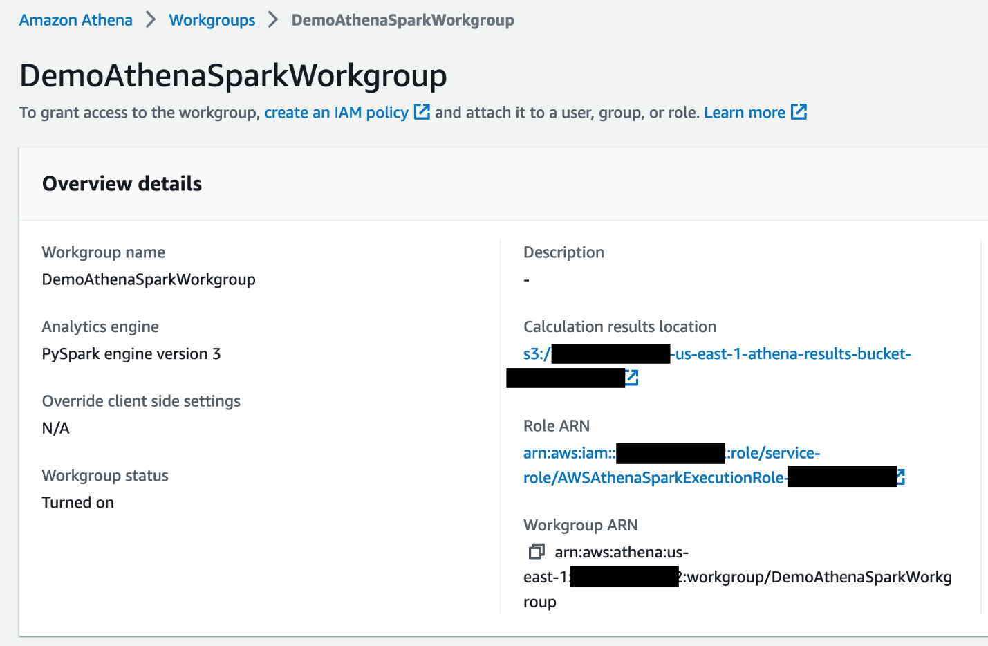
- An existing Athena workgroup configured with SQL engine
- An IAM user or role with the following permissions:
AmazonAthenaFullAccessmanaged policy- S3 Tables permissions for creating and managing table buckets
- S3 Tables permissions for creating and managing tables within buckets
- Read access to the public dataset location:
s3://aws-bigdata-blog/generated_synthetic_reviews/data/
You will create an S3 table bucket named athena-ctas-s3table-demo as part of this walkthrough. Make sure this name is available in your chosen AWS Region.
Set up a database and tables in Athena
Let’s start by creating a database and source table to hold our Parquet data. This table will serve as the data source for our CTAS operation.
Navigate to the Athena query editor to run the following queries:
Because the data is partitioned by product category, you must add the partition information to the table metadata using MSCK REPAIR TABLE:
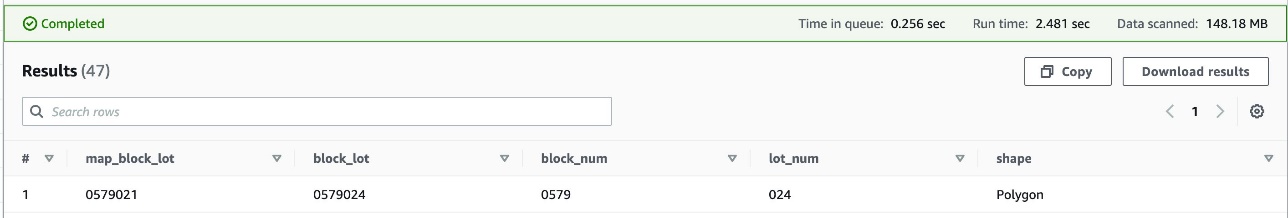
The preview query should return sample review data, confirming the table is ready for transformation:
Create a table bucket
Table buckets are designed to store tabular data and metadata as objects for analytics workloads. Follow these steps to create a table bucket:
- Sign in to the console in your preferred Region and open the Amazon S3 console.
- In the navigation pane, choose Table buckets.
- Choose Create table bucket.
- For Table bucket name, enter
athena-ctas-s3table-demo. - Select Enable integration for Integration with AWS analytics services if not already enabled.
- Leave the encryption option to default.
- Choose Create table bucket.
You can now see athena-ctas-s3table-demo listed under Table buckets.
Create a namespace
Namespaces provide logical organization for tables within your S3 table bucket, facilitating scalable table management. In this step, we create a reviews_namespace to organize our customer review tables. Follow these steps to create the table namespace:
- In the navigation pane under Table buckets, choose your newly created bucket
athena-ctas-s3table-demo. - On the bucket details page, choose Create table with Athena.
- Choose Create a namespace for Namespace configuration.
- Enter
reviews_namespacefor Namespace name. - Choose Create namespace.
- Choose Create table with Athena to navigate to the Athena query editor.
You should now see your S3 Tables configuration automatically selected under Data, as shown in the following screenshot.
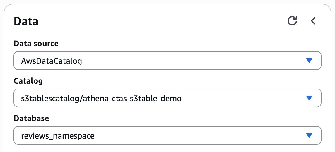
When you enable Integration with AWS analytics services, when creating an S3 table bucket, AWS Glue creates a new catalog called s3tablescatalog in your account’s default Data Catalog specific to your Region. The integration maps the S3 table bucket resources in your account and Region in this catalog.
This configuration makes sure subsequent queries will target your S3 Tables namespace. You’re now ready to create tables using the CTAS functionality.
Create a new S3 table using the customer_reviews table
A table represents a structured dataset consisting of underlying table data and related metadata stored in the Iceberg table format. In the following steps, we transform the customer_reviews table that we created earlier on the Parquet dataset into an S3 table using the Athena CTAS statement. We partition by date using the day() partition transforms from Iceberg.
Run the following CTAS query:
This query creates as S3 table with the following optimizations:
- Parquet format – Efficient columnar storage for analytics
- Day-level partitioning – Uses Iceberg’s
day()transform onreview_datefor fast queries when filtering on dates - Filtered data – Includes only reviews from 2016 onwards to demonstrate selective transformation
You have successfully transformed your Parquet dataset to S3 Tables using a single CTAS statement.
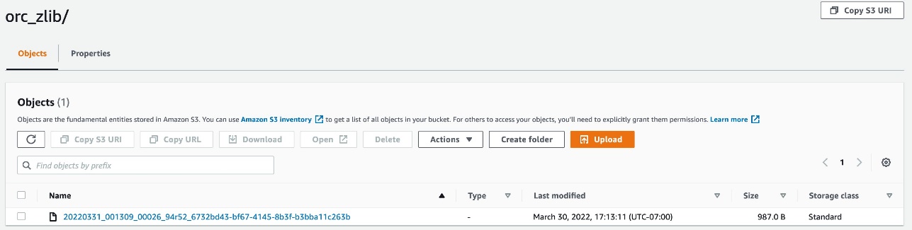
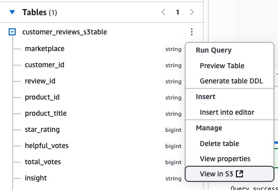
After you create the table, customer_reviews_s3table will appear under Tables in the Athena console. You can also view the table on the Amazon S3 console by choosing the options menu (three vertical dots) next to the table name and choosing View in S3.
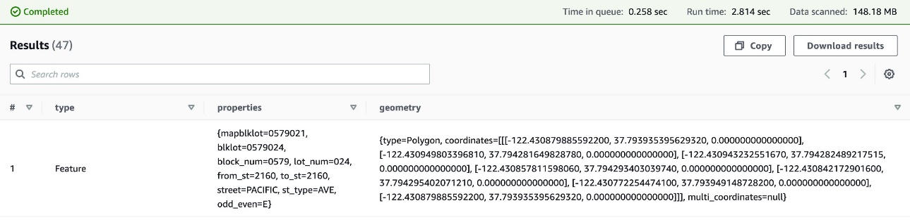
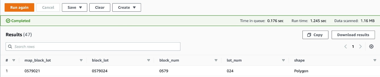
Run a preview query to confirm the data transformation:
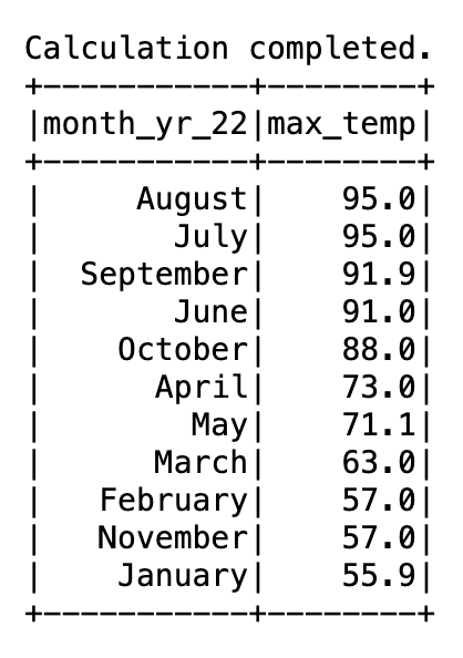
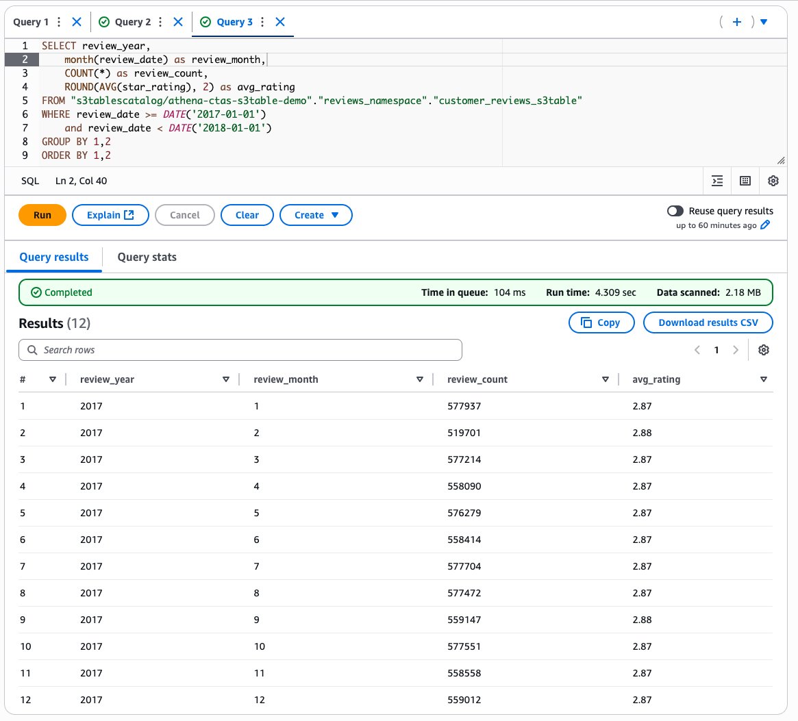
Next, let’s analyze monthly review trends:
The following screenshot shows our output.
ACID operations on S3 Tables
Athena supports standard SQL DML operations (INSERT, UPDATE, DELETE and MERGE INTO) on S3 Tables with full ACID transaction guarantees. Let’s demonstrate these capabilities by adding historical data and performing data quality checks.
Insert more data into the table using INSERT
Use the following query to insert review data from 2014 and 2015 that wasn’t included in the initial CTAS operation:
Check which years are now present in the table:
The following screenshot shows our output.
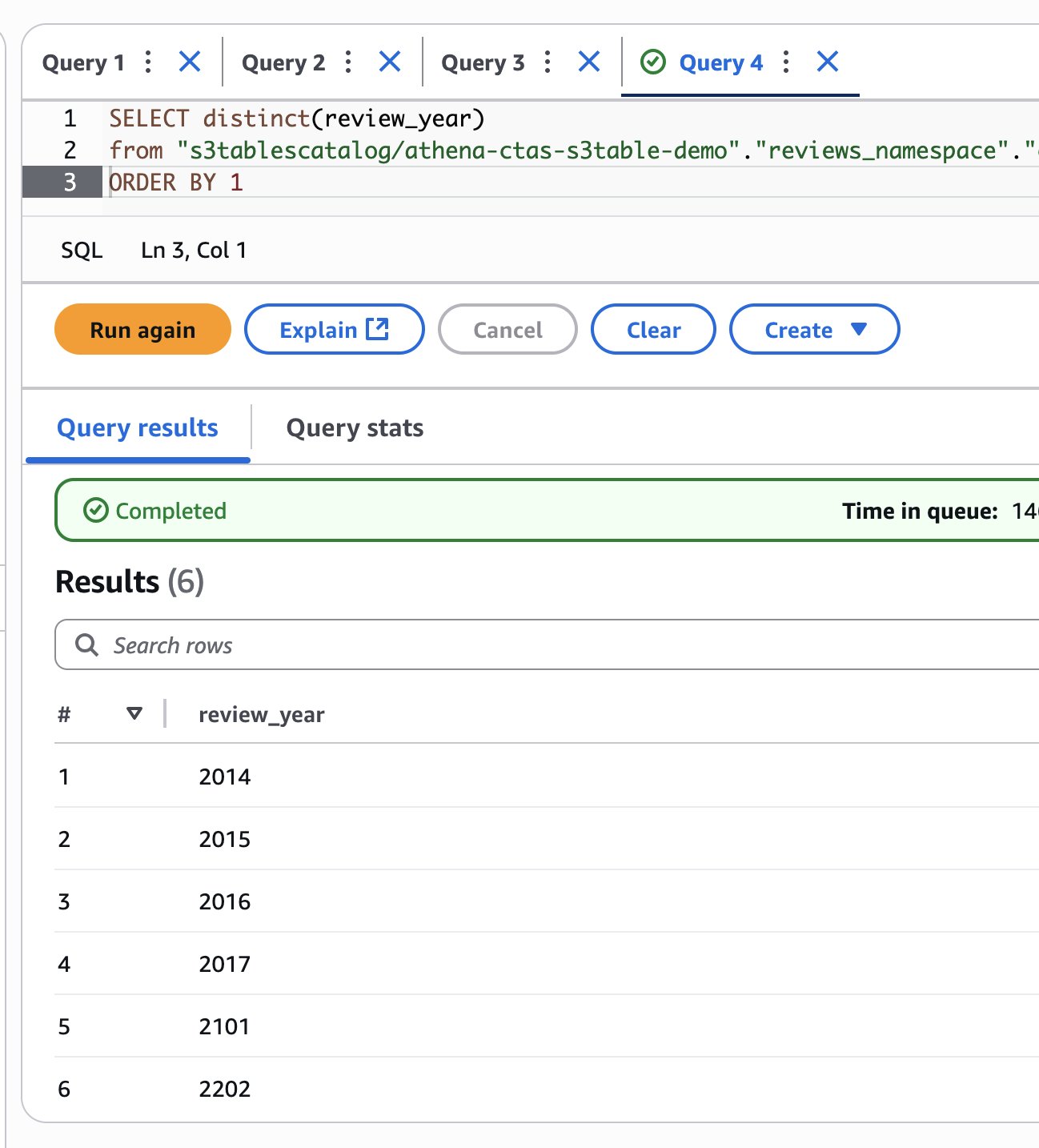
The results show that you have successfully added 2014 and 2015 data. However, you might also notice some invalid years like 2101 and 2202, which appear to be data quality issues in the source dataset.
Clean invalid data using DELETE
Remove the records with incorrect years using the S3 Tables DELETE capability:
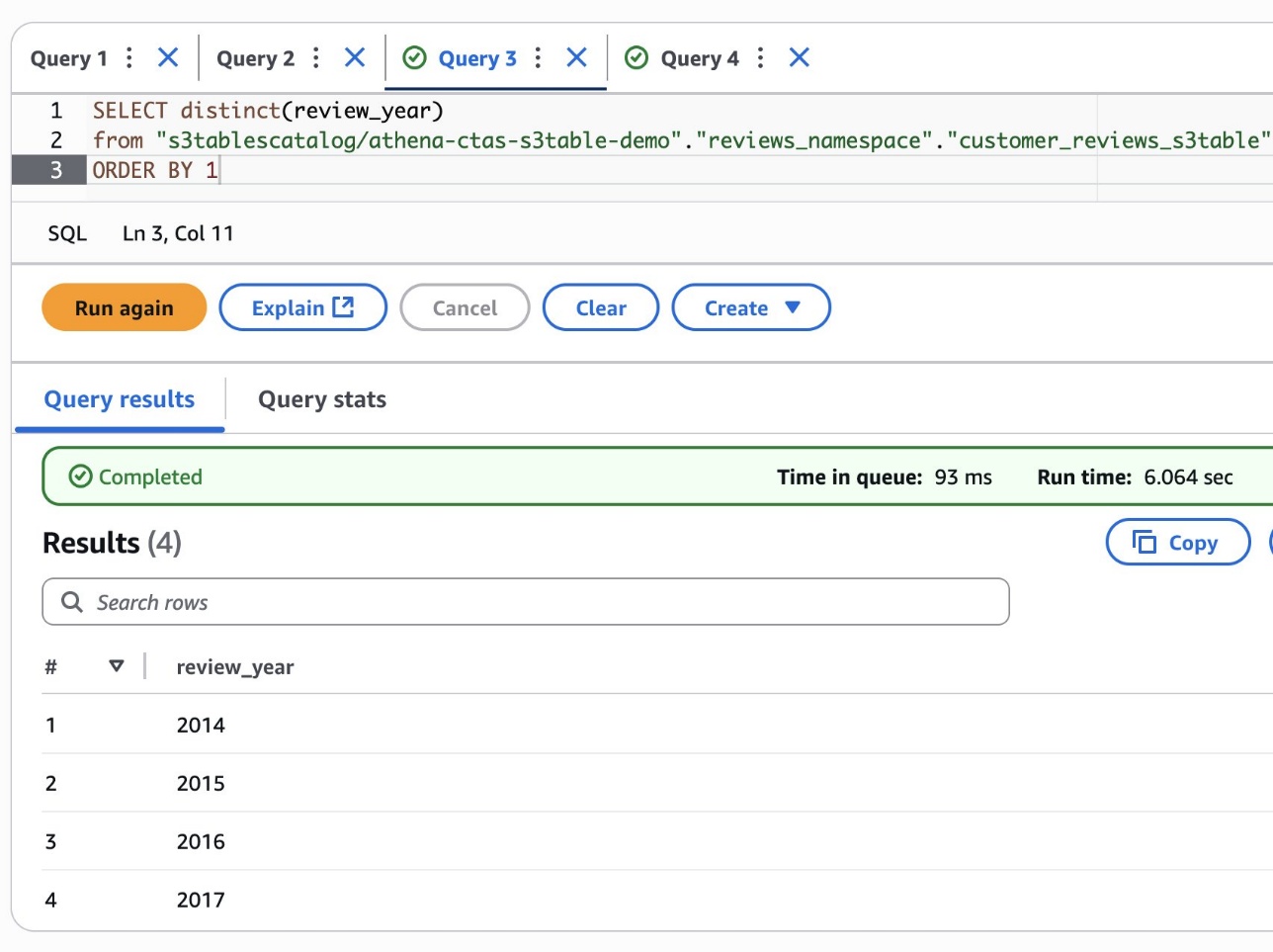
Confirm the invalid records have been removed.
Update product categories using UPDATE
Let’s demonstrate the UPDATE operation with a business scenario. Imagine the company decides to rebrand the Movies_TV product category to Entertainment_Media to better reflect customer preferences.
First, examine the current product categories and their record counts:
You should see a record with product_category as Movies_TV with approximately 5,690,101 reviews. Use the following query to update all Movies_TV records to the new category name:
Verify the category name change while confirming the record count remains the same:
The results now show Entertainment_Media with the same record count (5,690,101), confirming that the UPDATE operation successfully modified the category name while preserving data integrity.
These examples demonstrate transactional support in S3 Tables through Athena. Combined with automated table maintenance, this helps you build scalable, transactional data lakes more efficiently with minimal operational overhead.
Additional transformation scenarios using CTAS
The Athena CTAS functionality supports multiple transformation paths to S3 Tables. The following scenarios demonstrate how organizations can use this capability for various data modernization needs:
- Convert from various data formats – Athena can query data in a wide range of formats as well as federated data sources, and you can convert these queryable sources to an S3 table using CTAS. For example, to create an S3 table from a federated data source, use the following query:
- Transform between S3 tables for optimized analytics – Organizations often need to create derived tables from existing S3 tables optimized for specific query patterns. For example, consider a table containing detailed customer reviews that’s partitioned by product category. If your analytics team frequently queries by date ranges, you can use CTAS to create a new S3 table partitioned by date for significantly better performance on time-based queries. For example, the following query creates an aggregated analytics S3 table:
- Transform from self-managed open table formats – Organizations maintaining their own Iceberg tables can transform them into S3 tables to take advantage of automatic optimization and reduce operational overhead:
- Combine multiple source tables – Organizations often need to consolidate data from multiple tables into a single table for simplified analytics. This approach can help reduce query complexity and improve performance by pre-joining related datasets. The following query joins multiple tables using CTAS to create an S3 table:
These scenarios demonstrate the flexibility of Athena CTAS for various data modernization needs, from simple format conversions to complex data consolidation projects.
Clean up
To avoid ongoing charges, clean up the resources created during this walkthrough. Complete these steps in the specified order to facilitate proper resource deletion. You might need to add respective delete permissions for databases, table buckets, and tables if your IAM user or role doesn’t already have them.
- Delete the S3 table created through CTAS:
- Remove the namespace from the table bucket:
- Delete the table bucket.
- Remove the database and table created for the synthetic dataset:
- Delete any created IAM roles or policies.
- Delete the Athena query result location in Amazon S3 if you stored results in an S3 location.
Conclusion
This post demonstrated how the CTAS functionality in Athena simplifies data transformation to S3 Tables using standard SQL statements. We covered the complete transformation process, including format conversions, ACID operations, and various data transformation scenarios. The solution delivers simplified data transformation through single SQL statements, automatic maintenance, and seamless integration of S3 Tables with AWS analytics services and third-party tools. Organizations can modernize their data infrastructure while achieving enterprise-grade performance.
To get started, begin by identifying datasets that could benefit from optimization or transformation, then refer to Working with Amazon S3 Tables and table buckets and Register S3 table bucket catalogs and query Tables from Athena to implement the transformation patterns demonstrated in this walkthrough. The combination of the serverless capabilities of Athena with the automatic optimizations in S3 Tables can provide a powerful foundation for modern data analytics.
About the authors
 Pathik Shah is a Sr. Analytics Architect on Amazon Athena. He joined AWS in 2015 and has been focusing in the big data analytics space since then, helping customers build scalable and robust solutions using AWS Analytics services.
 Aritra Gupta is a Senior Technical Product Manager on the Amazon S3 team at Amazon Web Services. He helps customers build and scale data lakes. Based in Seattle, he likes to play chess and badminton in his spare time.


 Srividya Parthasarathy is a Senior Big Data Architect on the AWS Lake Formation team. She enjoys building data mesh solutions and sharing them with the community.
 Paul Villena is a Senior Analytics Solutions Architect in AWS with expertise in building modern data and analytics solutions to drive business value. He works with customers to help them harness the power of the cloud. His areas of interests are infrastructure as code, serverless technologies, and coding in Python.
 Derek Liu is a Senior Solutions Architect based out of Vancouver, BC. He enjoys helping customers solve big data challenges through AWS analytic services.


 Raj Devnath is a Product Manager at AWS on Amazon Athena. He is passionate about building products customers love and helping customers extract value from their data. His background is in delivering solutions for multiple end markets, such as finance, retail, smart buildings, home automation, and data communication systems.


 This will start a new session with the updated parameters.