Tag Archives: Amazon S3 Tables

Announcing replication support and Intelligent-Tiering for Amazon S3 Tables

Post Syndicated from Sébastien Stormacq original https://aws.amazon.com/blogs/aws/announcing-replication-support-and-intelligent-tiering-for-amazon-s3-tables/

Today, we’re announcing two new capabilities for Amazon S3 Tables: support for the new Intelligent-Tiering storage class that automatically optimizes costs based on access patterns, and replication support to automatically maintain consistent Apache Iceberg table replicas across AWS Regions and accounts without manual sync.

Organizations working with tabular data face two common challenges. First, they need to manually manage storage costs as their datasets grow and access patterns change over time. Second, when maintaining replicas of Iceberg tables across Regions or accounts, they must build and maintain complex architectures to track updates, manage object replication, and handle metadata transformations.

S3 Tables Intelligent-Tiering storage class
With the S3 Tables Intelligent-Tiering storage class, data is automatically tiered to the most cost-effective access tier based on access patterns. Data is stored in three low-latency tiers: Frequent Access, Infrequent Access (40% lower cost than Frequent Access), and Archive Instant Access (68% lower cost compared to Infrequent Access). After 30 days without access, data moves to Infrequent Access, and after 90 days, it moves to Archive Instant Access. This happens without changes to your applications or impact on performance.

Table maintenance activities, including compaction, snapshot expiration, and unreferenced file removal, operate without affecting the data’s access tiers. Compaction automatically processes only data in the Frequent Access tier, optimizing performance for actively queried data while reducing maintenance costs by skipping colder files in lower-cost tiers.

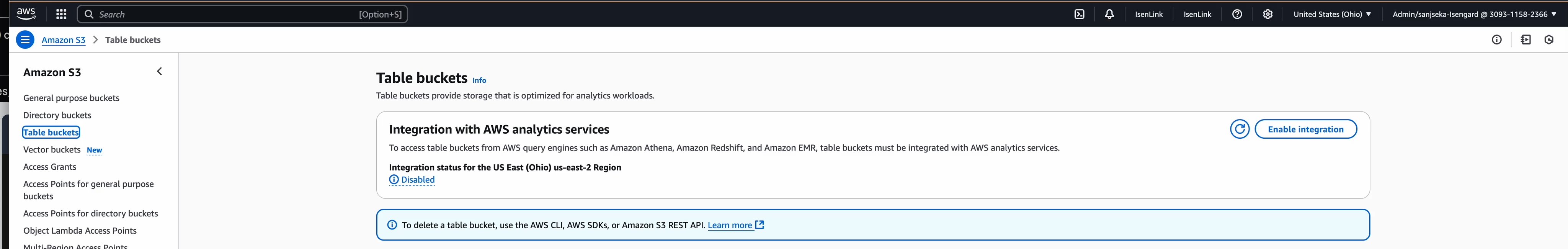
By default, all existing tables use the Standard storage class. When creating new tables, you can specify Intelligent-Tiering as the storage class, or you can rely on the default storage class configured at the table bucket level. You can set Intelligent-Tiering as the default storage class for your table bucket to automatically store tables in Intelligent-Tiering when no storage class is specified during creation.

Let me show you how it works
You can use the AWS Command Line Interface (AWS CLI) and the put-table-bucket-storage-class and get-table-bucket-storage-class commands to change or verify the storage tier of your S3 table bucket.

# Change the storage class
aws s3tables put-table-bucket-storage-class \
   --table-bucket-arn $TABLE_BUCKET_ARN  \
   --storage-class-configuration storageClass=INTELLIGENT_TIERING

# Verify the storage class
aws s3tables get-table-bucket-storage-class \
   --table-bucket-arn $TABLE_BUCKET_ARN  \

{ "storageClassConfiguration":
   { 
      "storageClass": "INTELLIGENT_TIERING"
   }
}

S3 Tables replication support
The new S3 Tables replication support helps you maintain consistent read replicas of your tables across AWS Regions and accounts. You specify the destination table bucket and the service creates read-only replica tables. It replicates all updates chronologically while preserving parent-child snapshot relationships. Table replication helps you build global datasets to minimize query latency for geographically distributed teams, meet compliance requirements, and provide data protection.

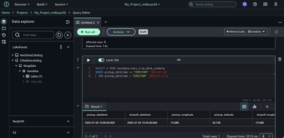
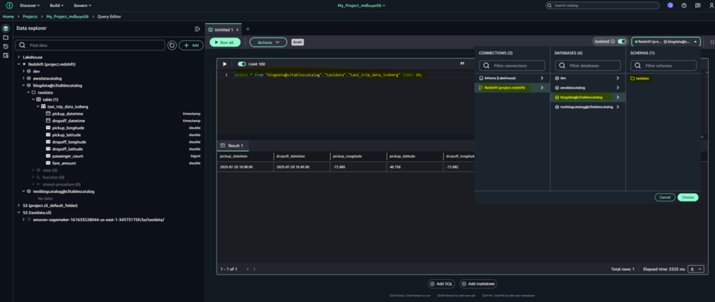
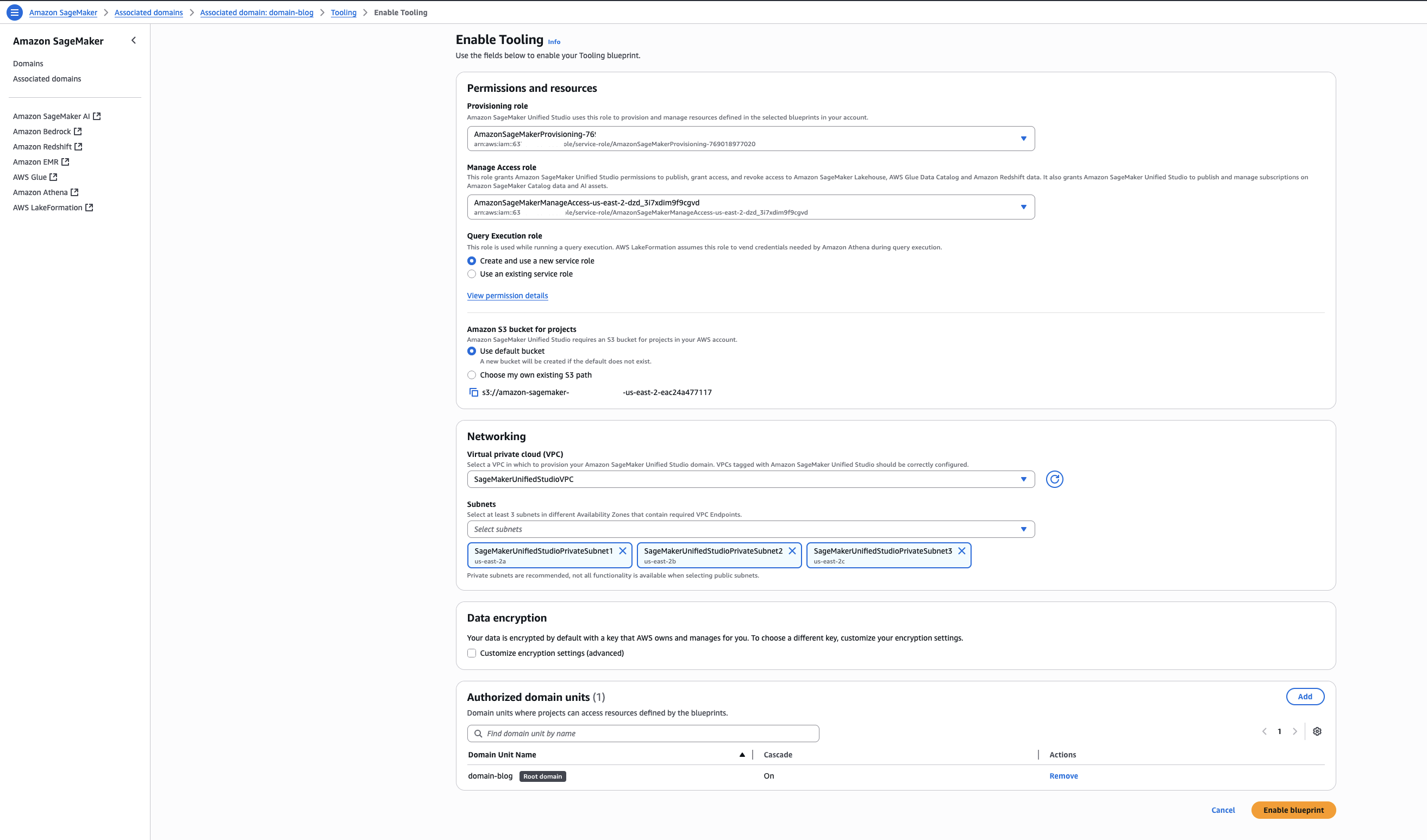
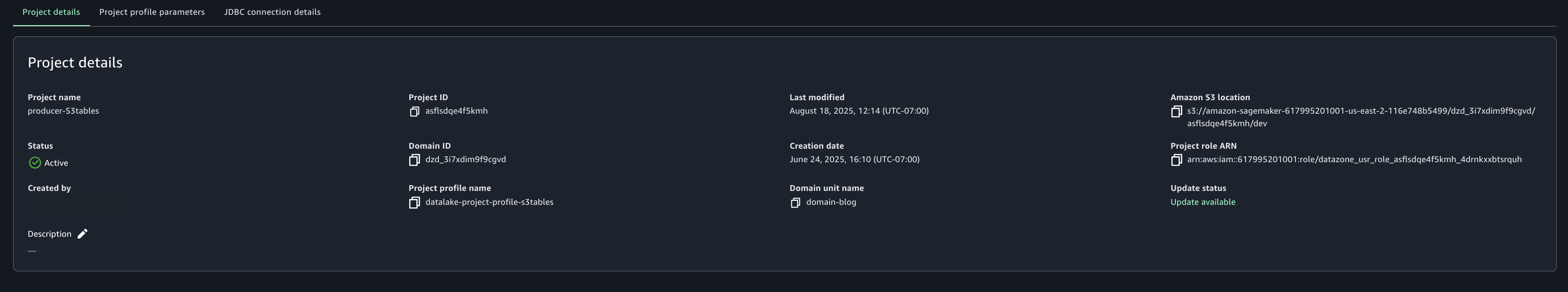
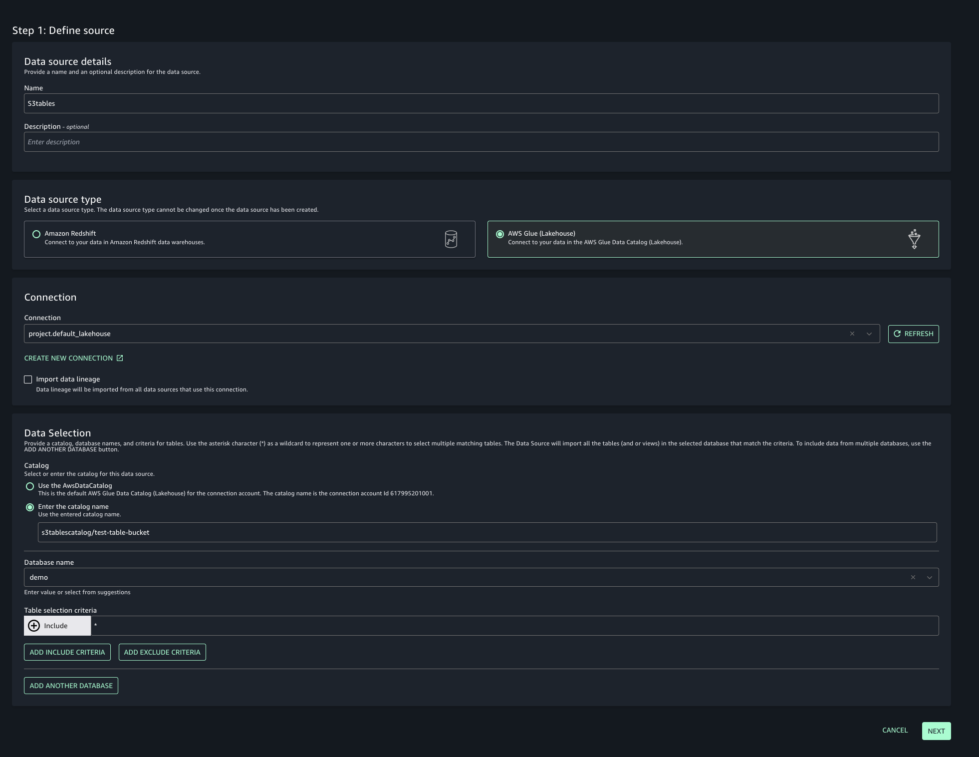
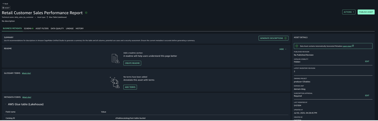
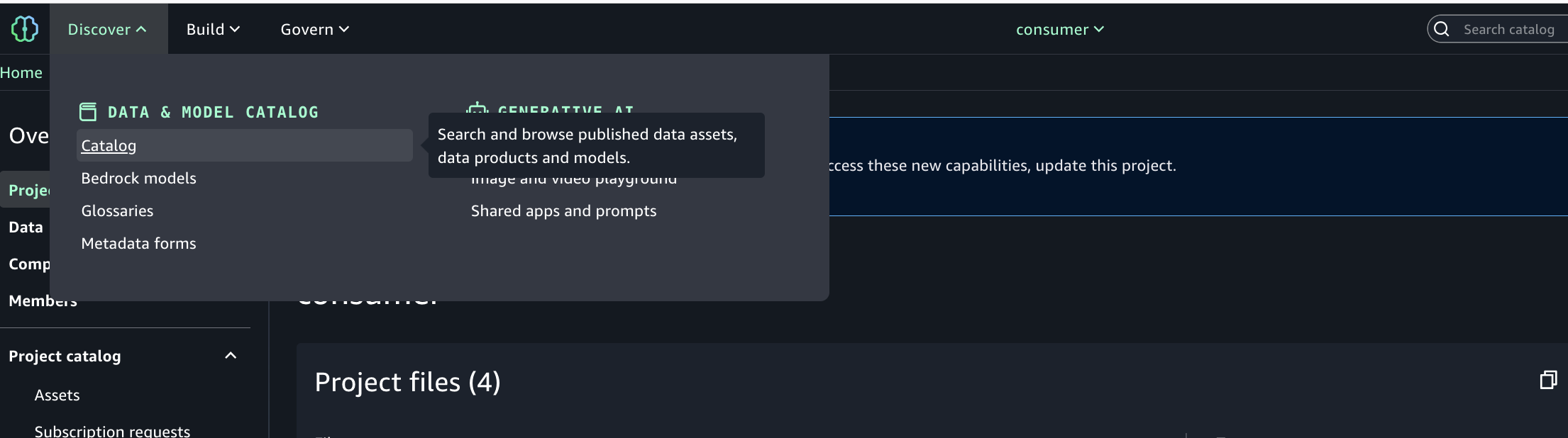
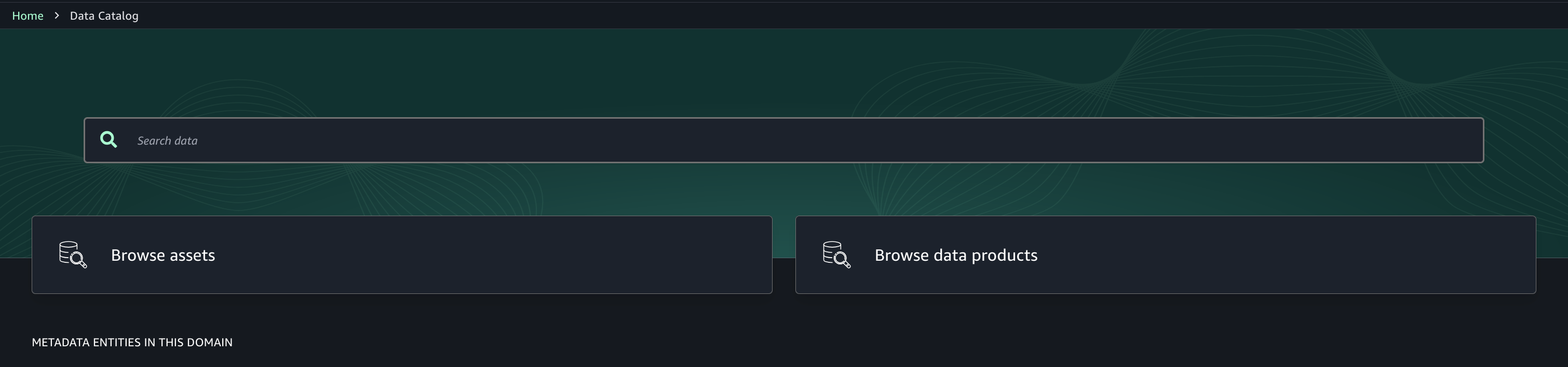
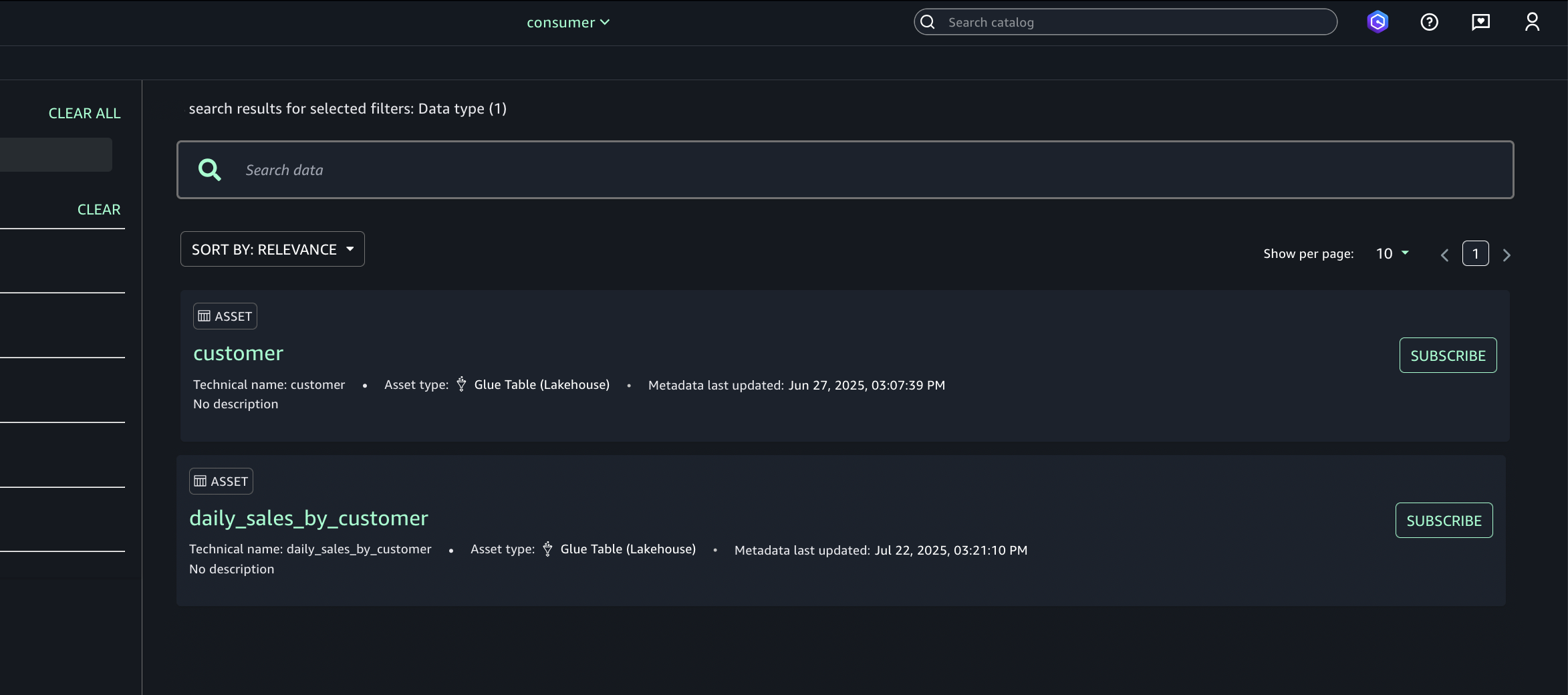
You can now easily create replica tables that deliver similar query performance as their source tables. Replica tables are updated within minutes of source table updates and support independent encryption and retention policies from their source tables. Replica tables can be queried using Amazon SageMaker Unified Studio or any Iceberg-compatible engine including DuckDB, PyIceberg, Apache Spark, and Trino.

You can create and maintain replicas of your tables through the AWS Management Console or APIs and AWS SDKs. You specify one or more destination table buckets to replicate your source tables. When you turn on replication, S3 Tables automatically creates read-only replica tables in your destination table buckets, backfills them with the latest state of the source table, and continually monitors for new updates to keep replicas in sync. This helps you meet time-travel and audit requirements while maintaining multiple replicas of your data.

Let me show you how it works
To show you how it works, I proceed in three steps. First, I create an S3 table bucket, create an Iceberg table, and populate it with data. Second, I configure the replication. Third, I connect to the replicated table and query the data to show you that changes are replicated.

For this demo, the S3 team kindly gave me access to an Amazon EMR cluster already provisioned. You can follow the Amazon EMR documentation to create your own cluster. They also created two S3 table buckets, a source and a destination for the replication. Again, the S3 Tables documentation will help you to get started.

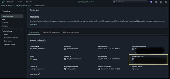
I take a note of the two S3 Tables bucket Amazon Resource Names (ARNs). In this demo, I refer to these as the environment variables SOURCE_TABLE_ARN and DEST_TABLE_ARN.

First step: Prepare the source database

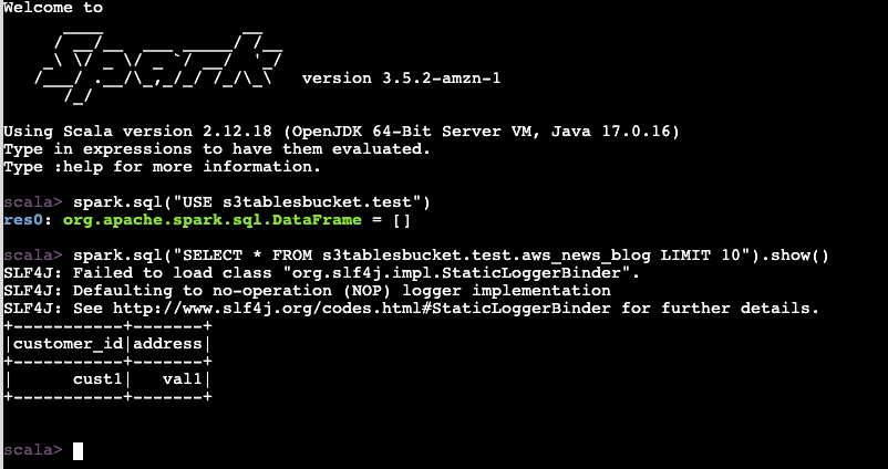
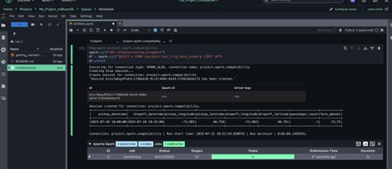
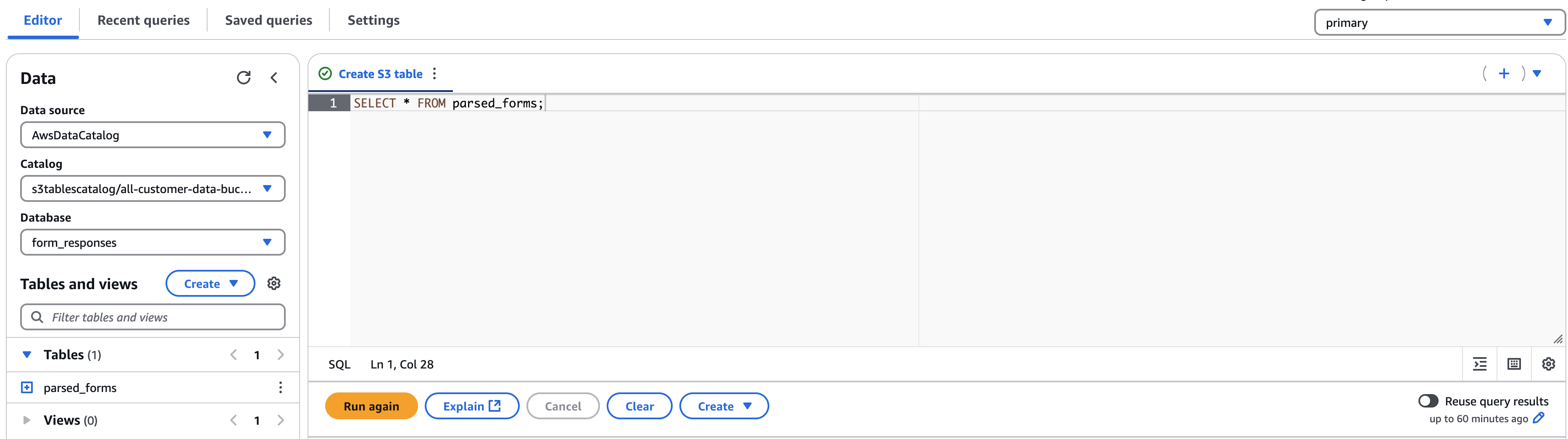
I start a terminal, connect to the EMR cluster, start a Spark session, create a table, and insert a row of data. The commands I use in this demo are documented in Accessing tables using the Amazon S3 Tables Iceberg REST endpoint.

sudo spark-shell \
--packages "org.apache.iceberg:iceberg-spark-runtime-3.5_2.12:1.4.1,software.amazon.awssdk:bundle:2.20.160,software.amazon.awssdk:url-connection-client:2.20.160" \
--master "local[*]" \
--conf "spark.sql.extensions=org.apache.iceberg.spark.extensions.IcebergSparkSessionExtensions" \
--conf "spark.sql.defaultCatalog=spark_catalog" \
--conf "spark.sql.catalog.spark_catalog=org.apache.iceberg.spark.SparkCatalog" \
--conf "spark.sql.catalog.spark_catalog.type=rest" \
--conf "spark.sql.catalog.spark_catalog.uri=https://s3tables.us-east-1.amazonaws.com/iceberg" \
--conf "spark.sql.catalog.spark_catalog.warehouse=arn:aws:s3tables:us-east-1:012345678901:bucket/aws-news-blog-test" \
--conf "spark.sql.catalog.spark_catalog.rest.sigv4-enabled=true" \
--conf "spark.sql.catalog.spark_catalog.rest.signing-name=s3tables" \
--conf "spark.sql.catalog.spark_catalog.rest.signing-region=us-east-1" \
--conf "spark.sql.catalog.spark_catalog.io-impl=org.apache.iceberg.aws.s3.S3FileIO" \
--conf "spark.hadoop.fs.s3a.aws.credentials.provider=org.apache.hadoop.fs.s3a.SimpleAWSCredentialProvider" \
--conf "spark.sql.catalog.spark_catalog.rest-metrics-reporting-enabled=false"

spark.sql("""
CREATE TABLE s3tablesbucket.test.aws_news_blog (
customer_id STRING,
address STRING
) USING iceberg
""")

spark.sql("INSERT INTO s3tablesbucket.test.aws_news_blog VALUES ('cust1', 'val1')")

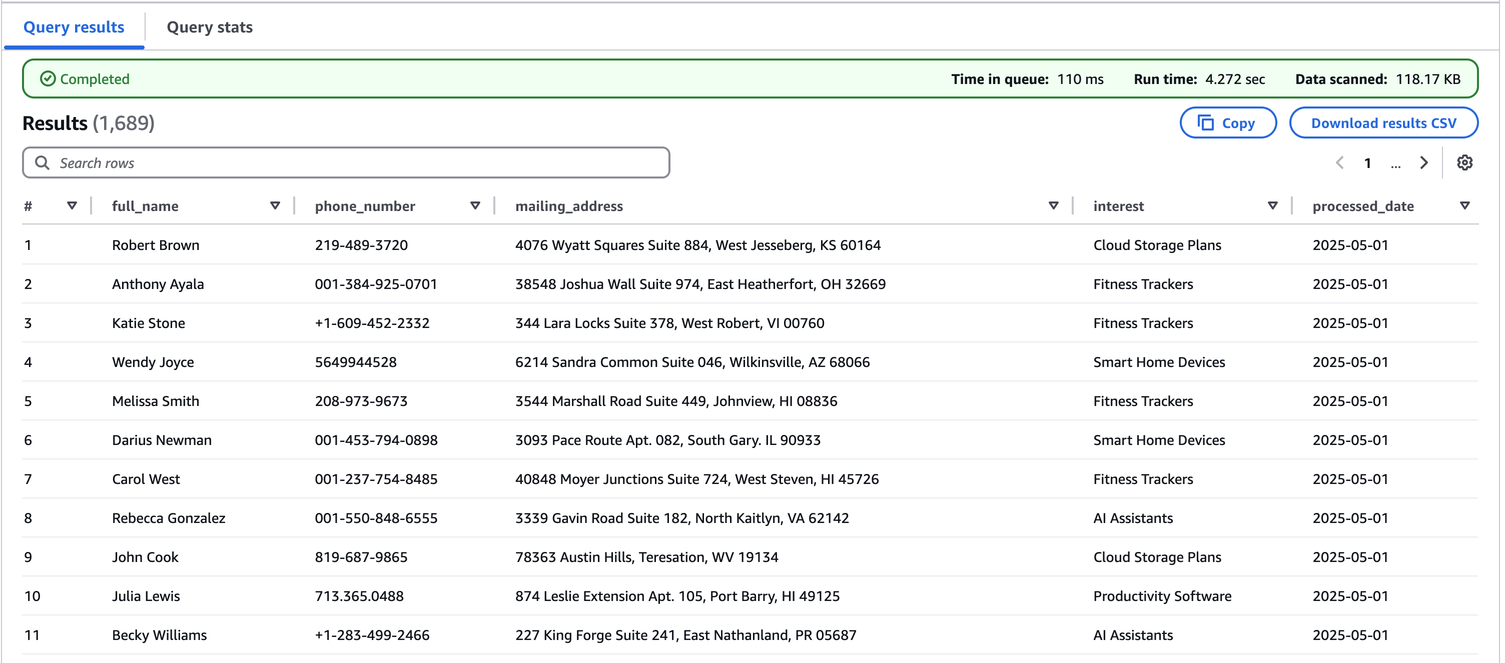
spark.sql("SELECT * FROM s3tablesbucket.test.aws_news_blog LIMIT 10").show()
+-----------+-------+
|customer_id|address|
+-----------+-------+
|      cust1|   val1|
+-----------+-------+

So far, so good.

Second step: Configure the replication for S3 Tables

Now, I use the CLI on my laptop to configure the S3 table bucket replication.

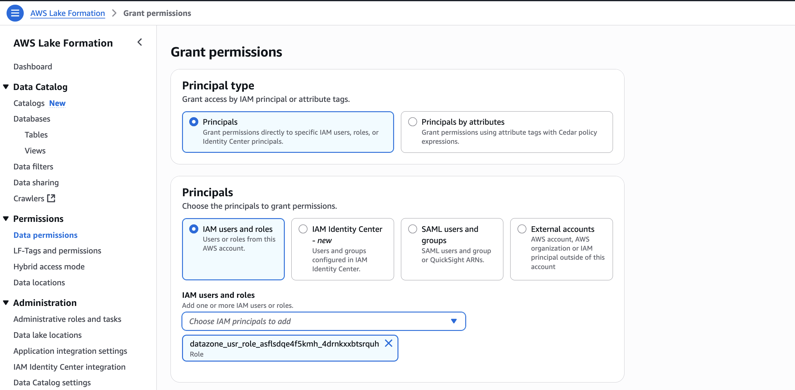
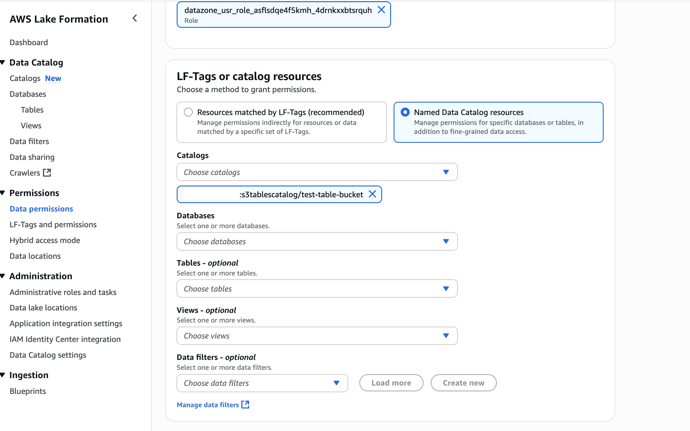
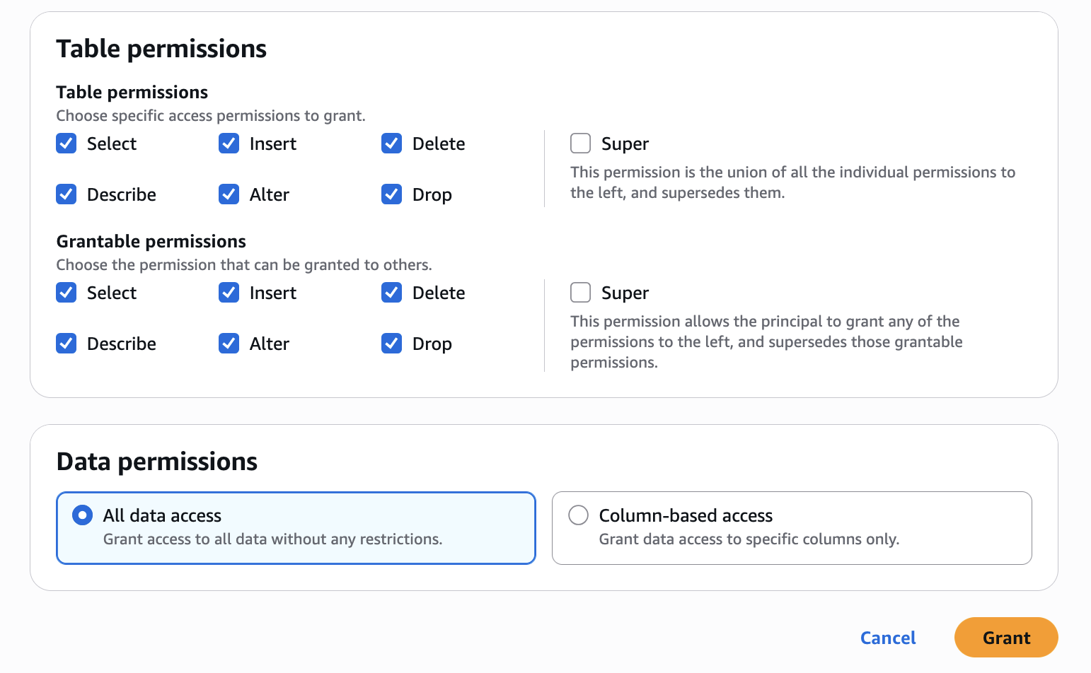
Before doing so, I create an AWS Identity and Access Management (IAM) policy to authorize the replication service to access my S3 table bucket and encryption keys. Refer to the S3 Tables replication documentation for the details. The permissions I used for this demo are:

{
    "Version": "2012-10-17",
    "Statement": [
        {
            "Effect": "Allow",
            "Action": [
                "s3:*",
                "s3tables:*",
                "kms:DescribeKey",
                "kms:GenerateDataKey",
                "kms:Decrypt"
            ],
            "Resource": "*"
        }
    ]
}

After having created this IAM policy, I can now proceed and configure the replication:

aws s3tables-replication put-table-replication \
--table-arn ${SOURCE_TABLE_ARN} \
--configuration  '{
    "role": "arn:aws:iam::<MY_ACCOUNT_NUMBER>:role/S3TableReplicationManualTestingRole", 
    "rules":[
        {
            "destinations": [
                {
                    "destinationTableBucketARN": "${DST_TABLE_ARN}"
                }]
        }
    ]

The replication starts automatically. Updates are typically replicated within minutes. The time it takes to complete depends on the volume of data in the source table.

Third step: Connect to the replicated table and query the data

Now, I connect to the EMR cluster again, and I start a second Spark session. This time, I use the destination table.

S3 Tables replication - destination table

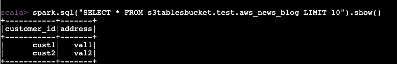
To verify the replication works, I insert a second row of data on the source table.

spark.sql("INSERT INTO s3tablesbucket.test.aws_news_blog VALUES ('cust2', 'val2')")

I wait a few minutes for the replication to trigger. I follow the status of the replication with the get-table-replication-status command.

aws s3tables-replication get-table-replication-status \
--table-arn ${SOURCE_TABLE_ARN} \
{
    "sourceTableArn": "arn:aws:s3tables:us-east-1:012345678901:bucket/manual-test/table/e0fce724-b758-4ee6-85f7-ca8bce556b41",
    "destinations": [
        {
            "replicationStatus": "pending",
            "destinationTableBucketArn": "arn:aws:s3tables:us-east-1:012345678901:bucket/manual-test-dst",
            "destinationTableArn": "arn:aws:s3tables:us-east-1:012345678901:bucket/manual-test-dst/table/5e3fb799-10dc-470d-a380-1a16d6716db0",
            "lastSuccessfulReplicatedUpdate": {
                "metadataLocation": "s3://e0fce724-b758-4ee6-8-i9tkzok34kum8fy6jpex5jn68cwf4use1b-s3alias/e0fce724-b758-4ee6-85f7-ca8bce556b41/metadata/00001-40a15eb3-d72d-43fe-a1cf-84b4b3934e4c.metadata.json",
                "timestamp": "2025-11-14T12:58:18.140281+00:00"
            }
        }
    ]
}

When replication status shows ready, I connect to the EMR cluster and I query the destination table. Without surprise, I see the new row of data.

S3 Tables replication - target table is up to date

Additional things to know
Here are a couple of additional points to pay attention to:

  • Replication for S3 Tables supports both Apache Iceberg V2 and V3 table formats, giving you flexibility in your table format choice.
  • You can configure replication at the table bucket level, making it straightforward to replicate all tables under that bucket without individual table configurations.
  • Your replica tables maintain the storage class you choose for your destination tables, which means you can optimize for your specific cost and performance needs.
  • Any Iceberg-compatible catalog can directly query your replica tables without additional coordination—they only need to point to the replica table location. This gives you flexibility in choosing query engines and tools.

Pricing and availability
You can track your storage usage by access tier through AWS Cost and Usage Reports and Amazon CloudWatch metrics. For replication monitoring, AWS CloudTrail logs provide events for each replicated object.

There are no additional charges to configure Intelligent-Tiering. You only pay for storage costs in each tier. Your tables continue to work as before, with automatic cost optimization based on your access patterns.

For S3 Tables replication, you pay the S3 Tables charges for storage in the destination table, for replication PUT requests, for table updates (commits), and for object monitoring on the replicated data. For cross-Region table replication, you also pay for inter-Region data transfer out from Amazon S3 to the destination Region based on the Region pair.

As usual, refer to the Amazon S3 pricing page for the details.

Both capabilities are available today in all AWS Regions where S3 Tables are supported.

To learn more about these new capabilities, visit the Amazon S3 Tables documentation or try them in the Amazon S3 console today. Share your feedback through AWS re:Post for Amazon S3 or through your AWS Support contacts.

— seb

Amazon S3 Storage Lens adds performance metrics, support for billions of prefixes, and export to S3 Tables

Post Syndicated from Veliswa Boya original https://aws.amazon.com/blogs/aws/amazon-s3-storage-lens-adds-performance-metrics-support-for-billions-of-prefixes-and-export-to-s3-tables/

Today, we’re announcing three new capabilities for Amazon S3 Storage Lens that give you deeper insights into your storage performance and usage patterns. With the addition of performance metrics, support for analyzing billions of prefixes, and direct export to Amazon S3 Tables, you have the tools you need to optimize application performance, reduce costs, and make data-driven decisions about your Amazon S3 storage strategy.

New performance metric categories
S3 Storage Lens now includes eight new performance metric categories that help identify and resolve performance constraints across your organization. These are available at organization, account, bucket, and prefix levels. For example, the service helps you identify small objects in a bucket or prefix that can  slow down application performance. This can be mitigated by batching small objects or using the Amazon S3 Express One Zone storage class for higher performance small object workloads.

To access the new performance metrics, you need to enable performance metrics in the S3 Storage Lens advanced tier when creating a new Storage Lens dashboard or editing an existing configuration.

Metric category Details Use case Mitigation
Read request size Distribution of read request sizes (GET) by day Identify dataset with small read request patterns that slow down performance Small request: Batch small objects or use Amazon S3 Express One Zone for high-performance small object workloads
Write request size Distribution of write request sizes (PUT, POST, COPY, and UploadPart) by day Identify dataset with small write request patterns that slow down performance Large request: Parallelize requests, use MPU or use AWS CRT
Storage size Distribution of object sizes Identify dataset with small small objects that slow down performance Small object sizes: Consider bundling small objects
Concurrent PUT 503 errors Number of 503s due to concurrent PUT operation on same object Identify prefixes with concurrent PUT throttling that slow down performance For single writer, modify retry behavior or use Amazon S3 Express One Zone. For multiple writers, use consensus mechanism or use Amazon S3 Express One Zone
Cross-Region data transfer Bytes transferred and requests sent across Region, in Region Identify potential performance and cost degradation due to cross-Region data access Co-locate compute with data in the same AWS Region
Unique objects accessed Number or percentage of unique objects accessed per day Identify datasets where small subset of objects are being frequently accessed. These can be moved to higher performance storage tier for better performance Consider moving active data to Amazon S3 Express One Zone or other caching solutions
FirstByteLatency (existing Amazon CloudWatch metric) Daily average of first byte latency metric The daily average per-request time from the complete request being received to when the response starts to be returned
TotalRequestLatency (existing Amazon CloudWatch metric) Daily average of Total Request Latency The daily average elapsed per request time from the first byte received to the last byte sent

How it works
On the Amazon S3 console I choose Create Storage Lens dashboard to create a new dashboard. You can also edit an existing dashboard configuration. I then configure general settings such as providing a Dashboard name, Status, and the optional Tags. Then, I choose Next.


Next, I define the scope of the dashboard by selecting Include all Regions and Include all buckets and specifying the Regions and buckets to be included.


I opt in to the Advanced tier in the Storage Lens dashboard configuration, select Performance metrics, then choose Next.


Next, I select Prefix aggregation as an additional metrics aggregation, then leave the rest of the information as default before I choose Next.


I select the Default metrics report, then General purpose bucket as the bucket type, and then select the Amazon S3 bucket in my AWS account as the Destination bucket. I leave the rest of the information as default, then select Next.


I review all the information before I choose Submit to finalize the process.


After it’s enabled, I’ll receive daily performance metrics directly in the Storage Lens console dashboard. You can also choose to export report in CSV or Parquet format to any bucket in your account or publish to Amazon CloudWatch. The performance metrics are aggregated and published daily and will be available at multiple levels: organization, account, bucket, and prefix. In this dropdown menu, I choose the % concurrent PUT 503 error for the Metric, Last 30 days for the Date range, and 10 for the Top N buckets.


The Concurrent PUT 503 error count metric tracks the number of 503 errors generated by simultaneous PUT operations to the same object. Throttling errors can degrade application performance. For a single writer, modify retry behavior or use higher performance storage tier such as Amazon S3 Express One Zone to mitigate concurrent PUT 503 errors. For multiple writers scenario, use a consensus mechanism to avoid concurrent PUT 503 errors or use higher performance storage tier such as Amazon S3 Express One Zone.

Complete analytics for all prefixes in your S3 buckets
S3 Storage Lens now supports analytics for all prefixes in your S3 buckets through a new Expanded prefixes metrics report. This capability removes previous limitations that restricted analysis to prefixes meeting a 1% size threshold and a maximum depth of 10 levels. You can now track up to billions of prefixes per bucket for analysis at the most granular prefix level, regardless of size or depth.

The Expanded prefixes metrics report includes all existing S3 Storage Lens metric categories: storage usage, activity metrics (requests and bytes transferred), data protection metrics, and detailed status code metrics.

How to get started
I follow the same steps outlined in the How it works section to create or update the Storage Lens dashboard. In Step 4 on the console, where you select export options, you can select the new Expanded prefixes metrics report. Thereafter, I can export the expanded prefixes metrics report in CSV or Parquet format to any general purpose bucket in my account for efficient querying of my Storage Lens data.


Good to know
This enhancement addresses scenarios where organizations need granular visibility across their entire prefix structure. For example, you can identify prefixes with incomplete multipart uploads to reduce costs, track compliance across your entire prefix structure for encryption and replication requirements, and detect performance issues at the most granular level.

Export S3 Storage Lens metrics to S3 Tables
S3 Storage Lens metrics can now be automatically exported to S3 Tables, a fully managed feature on AWS with built-in Apache Iceberg support. This integration provides daily automatic delivery of metrics to AWS managed S3 Tables for immediate querying without requiring additional processing infrastructure.

How to get started
I start by following the process outlined in Step 5 on the console, where I choose the export destination. This time, I choose Expanded prefixes metrics report. In addition to General purpose bucket, I choose Table bucket.

The new Storage Lens metrics are exported to new tables in an AWS managed bucket aws-s3.


I select the expanded_prefixes_activity_metrics table to view API usage metrics for expanded prefix reports.


I can preview the table on the Amazon S3 console or use Amazon Athena to query the table.


Good to know
S3 Tables integration with S3 Storage Lens simplifies metric analysis using familiar SQL tools and AWS analytics services such as Amazon Athena, Amazon QuickSight, Amazon EMR, and Amazon Redshift, without requiring a data pipeline. The metrics are automatically organized for optimal querying, with custom retention and encryption options to suit your needs.

This integration enables cross-account and cross-Region analysis, custom dashboard creation, and data correlation with other AWS services. For example, you can combine Storage Lens metrics with S3 Metadata to analyze prefix-level activity patterns and identify objects in prefixes with cold data that are eligible for transition to lower-cost storage tiers.

For your agentic AI workflows, you can use natural language to query S3 Storage Lens metrics in S3 Tables with the S3 Tables MCP Server. Agents can ask questions such as ‘which buckets grew the most last month?’ or ‘show me storage costs by storage class’ and get instant insights from your observability data.

Now available
All three enhancements are available in all AWS Regions where S3 Storage Lens is currently offered (except the China Regions and AWS GovCloud (US)).

These features are included in the Amazon S3 Storage Lens Advanced tier at no additional charge beyond standard advanced tier pricing. For the S3 Tables export, you pay only for S3 Tables storage, maintenance, and queries. There is no additional charge for the export functionality itself.

To learn more about Amazon S3 Storage Lens performance metrics, support for billions of prefixes, and export to S3 Tables, refer to the Amazon S3 user guide. For pricing details, visit the Amazon S3 pricing page.

Veliswa Boya.

Getting started with Apache Iceberg write support in Amazon Redshift

Post Syndicated from Sanket Hase original https://aws.amazon.com/blogs/big-data/getting-started-with-apache-iceberg-write-support-in-amazon-redshift/

Many companies store structured data in warehouses for analytics while keeping diverse datasets in data lakes for flexible processing. Until now, maintaining consistency between these systems required complex ETL processes and introduced potential data synchronization challenges.

The new Amazon Redshift Apache Iceberg write support removes these complexities through direct writes to Apache Iceberg tables stored in Amazon S3 and S3 Tables. With this native integration you can write data directly from Redshift queries to your data lake without intermediate ETL steps, facilitate data consistency with ACID-compliant transactions that help optimize query performance with flexible partitioning strategies, and use the familiar Redshift SQL interface when writing to Apache Iceberg tables. For example, you can now run a complex transformation in Redshift and write the results directly to an Apache Iceberg table that other analytics engines like Amazon EMR or Amazon Athena can immediately query. By using this approach you can query the same datasets from both Redshift and other analytics tools without copying data.

In this post, we show how you can use Amazon Redshift to write data directly to Apache Iceberg tables stored in Amazon S3 and S3 Tables for seamless integration between your data warehouse and data lake while maintaining ACID compliance.

“Verisk processes billions of catastrophe risk modeling records using Amazon Redshift and Apache Iceberg, achieving 30% faster query aggregations and significant storage cost reductions”

— Karthick Shanmugam, Associate Vice President, Verisk

Solution overview 

You can now create and write directly to Apache Iceberg tables stored in Amazon S3 and S3 Tables using familiar SQL commands in Amazon Redshift. We’ll guide you through configuring permissions for S3 table buckets using AWS Lake Formation. Finally, we’ll analyze customer and order datasets across both Redshift native and Apache Iceberg data formats to derive insights. The workflow is illustrated in the following diagram:

In this post we will walk you through following steps:

  1. Create an external database named customer_db in AWS Glue Data Catalog using Amazon Redshift SQL.
  2. Create an external table named customer in the Glue database and write customer data using Amazon Redshift SQL.
  3. Create table bucket named orders on Amazon S3 Tables to write orders data.
  4. Grant permissions using AWS Lake Formation to an IAM role for reading and writing to the orders table.
  5. Write orders data to the orders Amazon S3 table bucket.

This solution uses the following AWS services:

Prerequisites 

  • Create Amazon Redshift data warehouse (provisioned or Serverless).
  • Permissions to create database on AWS Glue Data Catalog from Redshift.
  • Create a new AWS Glue database called customer_db or use an existing database of your choice. If you use an existing database or a different name, replace customer_db with your actual database name in the subsequent commands.
  • S3 bucket and S3 Table bucket in the same AWS Region as your Redshift cluster.
  • Have access to an IAM role that is a Lake Formation data lake administrator. For instructions, refer to Create a data lake administrator.
  • Create IAM role RedshifticebergRole with following policy. Add managed permission for AmazonRedshiftQueryEditorV2.
    {
        "Version": "2012-10-17",
        "Statement": [
                        {
                            "Sid": "VisualEditor0",
                            "Effect": "Allow",
                            "Action": "redshift:GetClusterCredentialsWithIAM",
                            "Resource": "arn:aws:redshift:<YOUR-REGION>:<AWS-ACCOUNT-NUMBER>:dbname::<YOUR-REDSHIFT-CLUSTER-NAME>/*"
                        }
                    ]
    }

Setting up your environment

To set up your environment, complete the following steps.

Creating Apache Iceberg tables in Amazon S3 standard buckets

  1. Connect to Redshift using Query Editor V2.
  2. Create user for the Federated role RedshifticebergRole.
    Create user IAMR:RedshifticebergRole

  3. Verify you have an Amazon Redshift External Schema configured. Run following script on Redshift:
    CREATE EXTERNAL SCHEMA demo_iceberg
    FROM DATA CATALOG DATABASE 'customer_db'
    IAM_ROLE 'arn:aws:iam::<AWS-ACCOUNT-NUMBER>:role/RedshiftCustomizedIcebergRole';

  4. Create external table customer in Apache Iceberg table format in the demo_iceberg external schema created above and then insert data.

    Use this two-step approach when you need control over column definitions or plan to append data.

    Replace your S3 bucket name in place of <<your-bucket>>.

    -- Step 1: Define your table structure
    CREATE TABLE demo_iceberg.customer
    (
    customer_id bigint,
    customer_name varchar,
    email varchar,
    city varchar
    )
    USING ICEBERG
    LOCATION 's3://<<your-bucket>>/iceberg-data/customers/';
    
    -- Step 2: Insert data
                  
    (1, 'Customer1 Smith', '[email protected]', 'New York'),
    (2, 'Customer2 Johnson', '[email protected]', 'Los Angeles'),
    (3, 'Customer3 Brown', '[email protected]', 'Chicago'),
    (4, 'Customer4 Davis', '[email protected]', 'Houston'),
    (5, 'Customer5 Wilson', '[email protected]', 'Phoenix'),
    (6, 'Customer6 Miller', '[email protected]', 'Philadelphia'),
    (7, 'Customer7 Garcia', '[email protected]', 'San Antonio'),
    (8, 'Customer8 Rodriguez', '[email protected]', 'San Diego'),
    (9, 'Customer9 Martinez', '[email protected]', 'Dallas'),
    (10, 'Customer10 Anderson', '[email protected]', 'San Jose'),
    (11, 'Customer11 Taylor', '[email protected]', 'Austin'),
    (12, 'Customer12 Thomas', '[email protected]', 'Jacksonville'),
    (13, 'Customer13 Jackson', '[email protected]', 'Fort Worth'),
    (14, 'Customer14 White', '[email protected]', 'Columbus'),
    (15, 'Customer15 Harris', '[email protected]', 'Charlotte');
    
    -- Step 3: Select data
    SELECT * FROM demo_iceberg.customer;
    

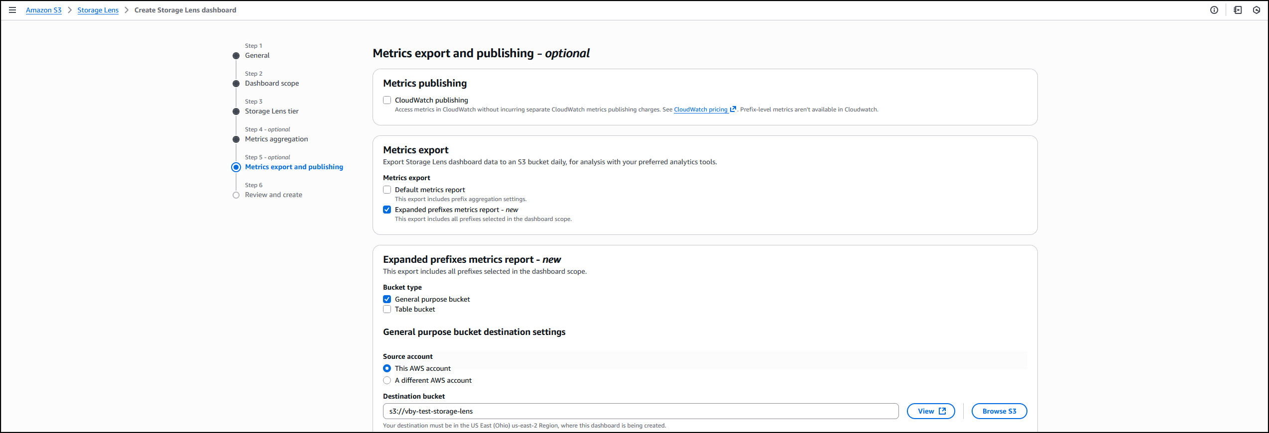
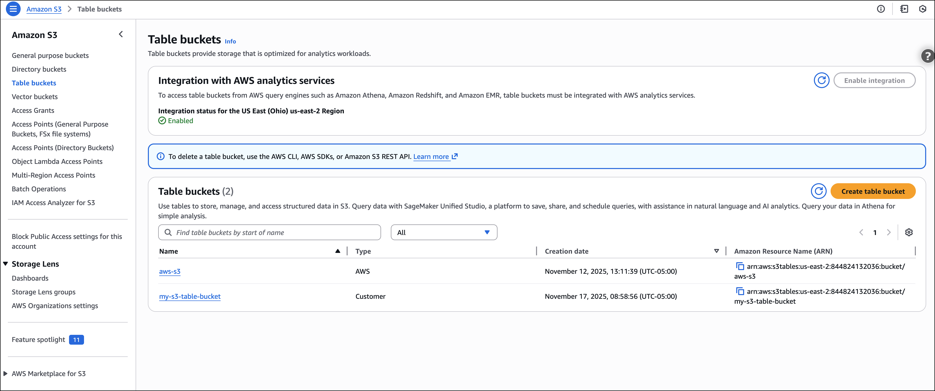
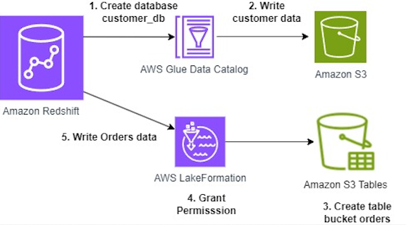
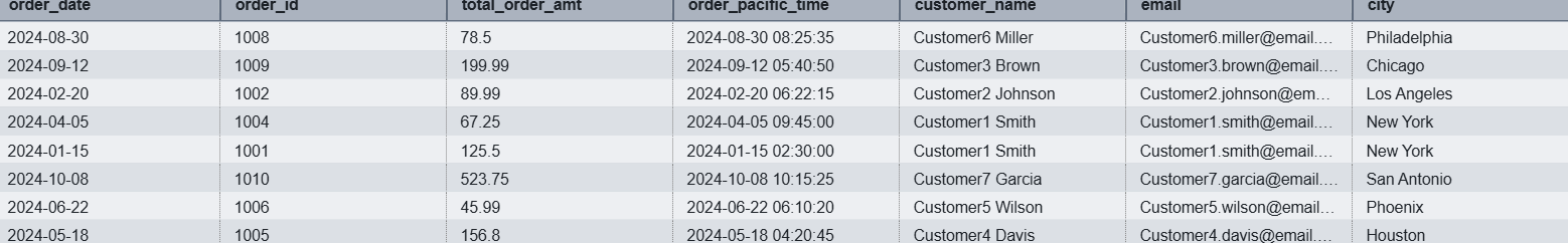
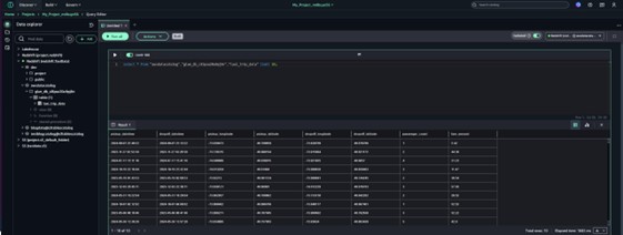
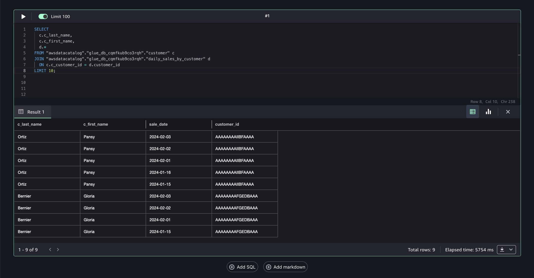
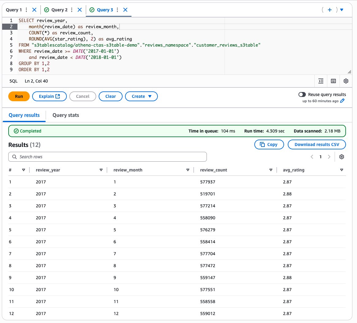
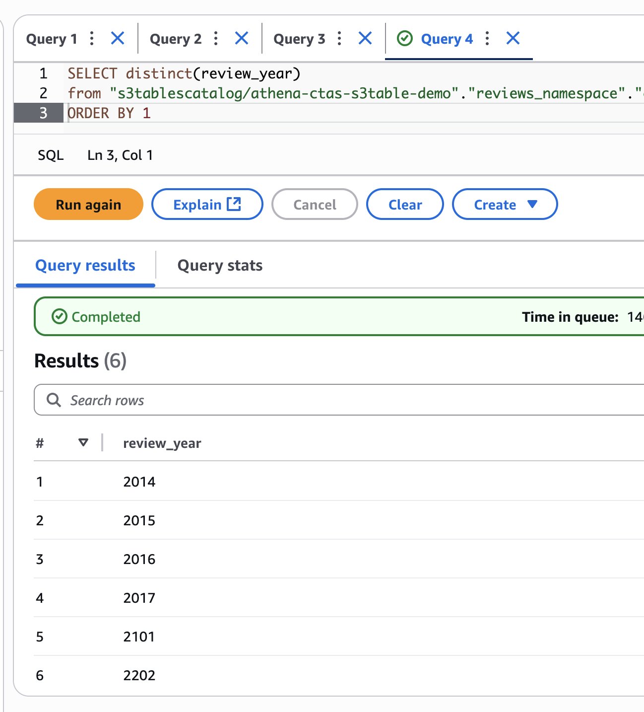
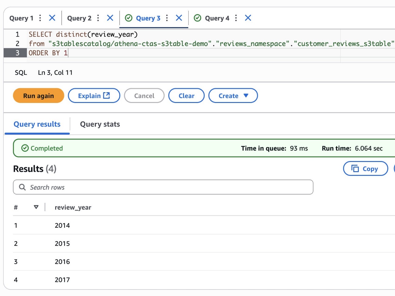
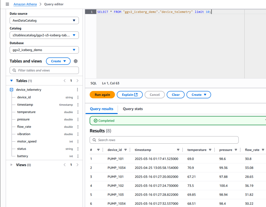
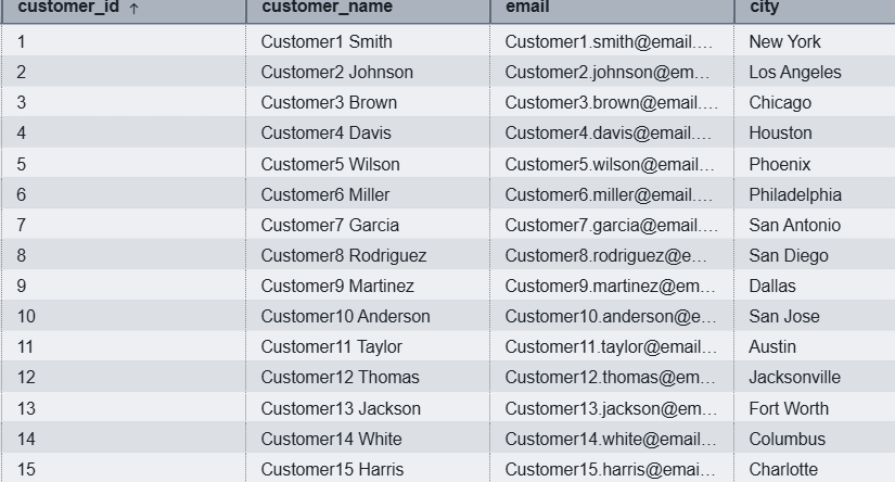
    Figure 2: Result from demo_iceberg.customer

  5. Grant access to external schema for user IAMR:RedshifticebergRole:
    Grant usage on schema demo_iceberg to "IAMR:RedshifticebergRole";

Create Apache Iceberg tables in Amazon S3 Table buckets

Amazon S3 table buckets are integrated with AWS Lake Formation, which serves as the central authority for managing data access permissions. When working with Apache Iceberg tables, Lake Formation provides a unified security framework that simplifies access control across your entire data lake. This centralized approach makes sure consistent and efficient permission management, alleviating the need to handle permissions in multiple places.

To create an S3 table bucket:

  1. Go to Amazon S3, choose Table buckets in the left navigation pane.
  2. On the Table buckets page, in the Integration with AWS analytics services section, choose Enable integration.
  3. In the Table buckets list, choose the Create table bucket button and enter a name for your table bucket, for example, iceberg-write-blog, and choose Create table bucket. After creation, the bucket will appear in the S3 tables catalog, s3tablescatalog, in the Lake Formation console.
  4. In the AWS Lake Formation console, choose Catalogs, in the Catalogs table select s3tablescatalog to open the detail page for that table.
  5. On the s3tablescatalog details page, under Catalogs, choose the table bucket iceberg-write-blog.
  6. On the iceberg-write-blog details page, under Databases, choose Create database.
  7. Enter the database name iceberg_write_namespace, select the Catalog from the drop down menu, and choose Create database.
  8. Grant a permission to create a table in the database to the Lake Formation IAM role. On the iceberg-write-blog details page select the radio button for iceberg_write_namespace, choose Actions, Grant.
  9. On the Grant permissions page, under Principal type select Principals, under Principals select IAM users and roles, in the IAM users and roles drop down menu select RedshifticebergRole.
  10. For LF-Tags or catalog resources, choose Named Data Catalog resources, for Catalogs select iceberg-write-blog and for Databases select iceberg_write_namespace.
  11. For Database permissions select the checkbox for Create table, Drop, and Describe, then choose Grant.

Creating Apache Iceberg tables in Amazon Redshift using Amazon S3 table buckets

AWS Lake Formation catalogs are automatically mounted on Amazon Redshift data warehouses in same account. Amazon Redshift writes directly to S3 Tables using the auto mounted S3 table catalog. The SQL syntax for writing to Apache Iceberg tables stored in S3 table buckets is similar to the syntax for Apache Iceberg tables stored in S3 standard buckets. The key difference is the auto mounted S3 Table catalog, which supports three-part notation access. This feature alleviates the need to create an EXTERNAL SCHEMA when referencing data lake Apache Iceberg tables residing in S3 Table buckets.

To create the Apache Iceberg table:

  1. Switch to the RedshifticebergRole. To access S3 tables through the Redshift Query Editor V2, you must use a Federated user account, the RedshifticebergRole has been granted the necessary Lake Formation permissions.
  2. Log in to Redshift using the Query Editor V2 Federated user option.
  3. In Query Editor V2, create the table named orders in Apache Iceberg table format:
    CREATE TABLE "iceberg-write-blog@s3tablescatalog".iceberg_write_namespace.orders
    (
     customer_id BIGINT,
     order_id BIGINT,
     Total_order_amt DECIMAL(10,2),
     Total_order_tax_amt REAL,
     tax_pct DOUBLE PRECISION,
     order_date DATE,
     order_created_at_tz TIMESTAMPTZ,
     is_active_ind BOOLEAN
    )
    USING ICEBERG 
    PARTITIONED BY (DAY(order_date));
    

  4. Insert data into the table using standard SQL:
    INSERT INTO "iceberg-write-blog@s3tablescatalog".iceberg_write_namespace.orders
    (order_date, order_id, customer_id, total_order_amt, total_order_tax_amt, tax_pct, order_created_at_tz, is_active_ind)
    VALUES
    ('2024-01-15', 1001, 1, 125.50, 10.04, 0.08, '2024-01-15 10:30:00-06:00', true),
    ('2024-02-20', 1002, 2, 89.99, 6.75, 0.075, '2024-02-20 14:22:15-06:00', true),
    ('2024-03-10', 1003, 3, 234.75, 20.78, 0.0885, '2024-03-10 09:15:30-06:00', false),
    ('2024-04-05', 1004, 1, 67.25, 5.38, 0.08, '2024-04-05 16:45:00-05:00', true),
    ('2024-05-18', 1005, 4, 156.80, 12.54, 0.08, '2024-05-18 11:20:45-05:00', true),
    ('2024-06-22', 1006, 5, 45.99, 4.14, 0.09, '2024-06-22 13:10:20-05:00', true),
    ('2024-07-14', 1007, 2, 312.40, 24.99, 0.08, '2024-07-14 08:35:10-05:00', false),
    ('2024-08-30', 1008, 6, 78.50, 7.07, 0.09, '2024-08-30 15:25:35-05:00', true),
    ('2024-09-12', 1009, 3, 199.99, 18.00, 0.09, '2024-09-12 12:40:50-05:00', true),
    ('2024-10-08', 1010, 7, 523.75, 41.90, 0.08, '2024-10-08 17:15:25-05:00', true),
    ('2024-10-25', 1011, 4, 92.30, 8.31, 0.09, '2024-10-25 10:05:15-05:00', false),
    ('2024-11-02', 1012, 8, 167.45, 13.40, 0.08, '2024-11-02 14:50:40-06:00', true),
    ('2024-11-08', 1013, 1, 34.99, 2.80, 0.08, '2024-11-08 09:30:20-06:00', true),
    ('2024-11-09', 1014, 9, 445.60, 40.10, 0.09, '2024-11-09 16:20:55-06:00', true),
    ('2024-11-10', 1015, 5, 278.85, 22.31, 0.08, '2024-11-10 11:45:30-06:00', true);
    

  5. Create a Redshift local_orders table and insert sample records:
    CREATE TABLE dev.public.local_orders
    (
    customer_id BIGINT,
    order_id BIGINT,
    Total_order_amt DECIMAL(10,2),
    Total_order_tax_amt REAL,
    tax_pct DOUBLE PRECISION,
    order_date DATE,
    order_created_at_tz TIMESTAMPTZ,
    is_active_ind BOOLEAN
    );
    
    
    INSERT INTO dev.public.local_orders
    (customer_id, order_id, Total_order_amt, Total_order_tax_amt, tax_pct, order_date, order_created_at_tz, is_active_ind)
    VALUES
    (1001, 5001, 299.99, 24.00, 0.08, '2024-01-15', '2024-01-15 14:30:00-05:00', true),
    (1002, 5002, 1250.50, 100.04, 0.08, '2024-01-16', '2024-01-16 09:15:22-05:00', true),
    (1003, 5003, 75.25, 6.02, 0.08, '2024-01-16', '2024-01-16 16:45:33-05:00', true),
    (1004, 5004, 499.99, 40.00, 0.08, '2024-01-17', '2024-01-17 11:20:45-05:00', true),
    (1005, 5005, 149.50, 11.96, 0.08, '2024-01-17', '2024-01-17 13:55:12-05:00', false),
    (1002, 5006, 899.99, 72.00, 0.08, '2024-01-18', '2024-01-18 10:05:30-05:00', true),
    (1006, 5007, 45.75, 3.66, 0.08, '2024-01-18', '2024-01-18 15:40:18-05:00', true),
    (1007, 5008, 1500.00, 120.00, 0.08, '2024-01-19', '2024-01-19 08:25:55-05:00', true),
    (1008, 5009, 250.25, 20.02, 0.08, '2024-01-19', '2024-01-19 12:10:40-05:00', true),
    (1009, 5010, 725.75, 58.06, 0.08, '2024-01-20', '2024-01-20 14:15:28-05:00', true);
    

  6. Using the CREATE TABLE AS (CTAS) format, create a table from the existing table with no compression:
    CREATE TABLE "iceberg-write-blog@s3tablescatalog".iceberg_write_namespace.orders_new 
    using ICEBERG
    TABLE PROPERTIES ('compression_type'='uncompressed')
    AS
    select * from dev.public.local_orders;
    

  7. Select data with standard SQL using the three-part notation:
    select * from "iceberg-write-blog@s3tablescatalog".iceberg_write_namespace.orders;

    You can also use the USE clause to specify the default database (and omit the database name):

    USE "iceberg-write-blog@s3tablescatalog";
    
    select * from iceberg_write_namespace.orders;

    The resulting table will look like the following image:

  8. Set a schema search path to further simplify table access by omitting the schema name from the notation:
    -- Redshift default database is set to 'iceberg-write-blog@s3tablescatalog'
    USE "iceberg-write-blog@s3tablescatalog";
    
    -- Redshift will search 'iceberg_write_namespace' to resolve table orders
    set search_path to iceberg_write_namespace;
    
    select * from orders;

  9. Show table:
    show table "iceberg-write-blog@s3tablescatalog".iceberg_write_namespace.orders 
    
    --Result
    CREATE TABLE "iceberg-write-blog@s3tablescatalog".iceberg_write_namespace.orders 
    (
    customer_id bigint,
    order_id bigint,
    total_order_amt decimal(10, 2),
    total_order_tax_amt float,
    tax_pct double precision,
    order_date date,
    order_created_at_tz timestamptz,
    is_active_ind Boolean
    )
    USING ICEBERG
    PARTITIONED BY (DAY(order_date))
    TABLE PROPERTIES ('compression_type'='snappy');

Bringing it together

Let’s demonstrate how to combine data from two sources and show how they can work together in a single query.

  • Customer data stored in standard S3 buckets
  • Orders data stored in S3 table buckets
  1. Log in to Redshift using Federated user:
    select 
    b.order_date,
    b.order_id,
    b.total_order_amt,
    CONVERT_TIMEZONE('America/Los_Angeles', b.order_created_at_tz) AS order_pacific_time,
    a.customer_name,
    a.email,
    a.city
    from dev.demo_iceberg.customer a join "iceberg-write-blog@s3tablescatalog".iceberg_write_namespace.orders b
    on(a.customer_id = b.customer_id)
    where b.order_date between '2024-01-15' and '2024-10-25'
    and b.is_active_ind=true;

    The result from the consolidated query:

  2. Drop table:
    Drop TABLE "iceberg-write-blog@s3tablescatalog".iceberg_write_namespace.orders_new;

Clean up

To avoid ongoing charges, follow these steps in order:

  1. Drop Apache Iceberg tables:
    DROP TABLE dev.demo_iceberg.customer;
    DROP TABLE "iceberg-write-blog@s3tablescatalog".iceberg_write_namespace.orders;

  2. Remove S3 objects, replace your-bucket with the name of the bucket you created:
    aws s3 rm s3://<your-bucket>/iceberg/ --recursive

  3. Remove Lake Formation permissions, replace your-bucket with the name of the bucket you created:
    aws lakeformation deregister-resource --resource-arn arn:aws:s3:::<your-bucket>

Conclusion

With Apache Iceberg write support in Amazon Redshift you can to build flexible data architectures that combine the performance of a data warehouse with the scalability of a data lake. You can now write data directly to Apache Iceberg tables while maintaining ACID compliance and partitioning for query optimization. You can use Amazon Redshift to create Apache Iceberg tables in your data lake, making them immediately queryable through Amazon EMR or Amazon Athena.

To learn more, review the Amazon Redshift Iceberg integration and Writing to Apache Iceberg tables documentation. Visit the AWS Database Blog for latest updates.


About the authors

Sanket Hase

Sanket Hase

Sanket is an Engineering Manager with the Amazon Redshift team, leading query execution teams in the areas of data lake analytics, hardware-software co-design, and vectorized query execution.

Harshida Patel

Harshida Patel

Harshida is a Principal Solutions Architect, Analytics with AWS.

Ritesh Kumar Sinha

Ritesh Kumar Sinha

Ritesh is an Analytics Specialist Solutions Architect based out of San Francisco. He has helped customers build scalable data warehousing and big data solutions for over 16 years. He loves to design and build efficient end-to-end solutions on AWS. In his spare time, he loves reading, walking, and doing yoga.

Raghu Kuppala

Raghu Kuppala

Raghu is an Analytics Specialist Solutions Architect experienced working in the databases, data warehousing, and analytics space. Outside of work, he enjoys trying different cuisines and spending time with his family and friends.

Xiening Dai

Xiening Dai

Xiening is a Principal Software Engineer working on Redshift Query Processing and Data Lake.

Getting started with Amazon S3 Tables in Amazon SageMaker Unified Studio

Post Syndicated from David Pasha original https://aws.amazon.com/blogs/big-data/getting-started-with-amazon-s3-tables-in-amazon-sagemaker-unified-studio/

Modern data teams face a critical challenge: their analytical datasets are scattered across multiple storage systems and formats, creating operational complexity that slows down insights and hampers collaboration. Data scientists waste valuable time navigating between different tools to access data stored in various locations, while data engineers struggle to maintain consistent performance and governance across disparate storage solutions. Teams often find themselves locked into specific query engines or analytics tools based on where their data resides, limiting their ability to choose the best tool for each analytical task.

Amazon SageMaker Unified Studio addresses this fragmentation by providing a single environment where teams can access and analyze organizational data using AWS analytics and AI/ML services. The new Amazon S3 Tables integration solves a fundamental problem: it enables teams to store their data in a unified, high-performance table format while maintaining the flexibility to query that same data seamlessly across multiple analytics engines—whether through JupyterLab notebooks, Amazon Redshift, Amazon Athena, or other integrated services. This eliminates the need to duplicate data or compromise on tool choice, allowing teams to focus on generating insights rather than managing data infrastructure complexity.

Table buckets are the third type of S3 bucket, taking place alongside the existing general purpose buckets, directory buckets, and now the fourth type – vector buckets. You can think of a table bucket as an analytics warehouse that can store Apache Iceberg tables with various schemas. Additionally, S3 Tables deliver the same durability, availability, scalability, and performance characteristics as S3 itself, and automatically optimize your storage to maximize query performance and to minimize cost.

In this post, you learn how to integrate SageMaker Unified Studio with S3 tables and query your data using Athena, Redshift, or Apache Spark in EMR and Glue.

Integrating S3 Tables with AWS analytics services

S3 table buckets integrate with AWS Glue Data Catalog and AWS Lake Formation to allow AWS analytics services to automatically discover and access your table data. For more information, see creating an S3 Tables catalog.

Before you get started with SageMaker Unified Studio, your administrator must first create a domain in the SageMaker Unified Studio and provide you with the URL. For more information, see the SageMaker Unified Studio Administrator Guide.

If you’ve never used S3 Tables in SageMaker Studio, you can allow it to enable the S3 Tables analytics integration when you create a new S3 Tables catalog in SageMaker Unified Studio.

Note: This integration needs to be configured individually in each AWS Region.

When you integrate using SageMaker Unified Studio, it takes the following actions in your account:

  • Creates a new AWS Identity and Access Management (IAM) service role that gives AWS Lake Formation access to all your tables and table buckets in the same AWS Region where you are going to provision the resources. This allows Lake Formation to manage access, permissions, and governance for all current and future table buckets.
  • Creates a catalog from an S3 table bucket in the AWS Glue Data Catalog.
  • Add the Redshift service role (AWSServiceRoleForRedshift) as a Lake Formation Read-only administrator permissions.

Prerequisites

Creating catalogs from S3 table buckets in SageMaker Unified Studio

To get started using S3 Tables in SageMaker Unified Studio you create a new Lakehouse catalog with S3 table bucket source using the following steps.

  1. Open the SageMaker console and use the region selector in the top navigation bar to choose the appropriate AWS Region.
  2. Select your SageMaker domain.
  3. Select or create a new project you want to create a table bucket in.
  4. In the navigation menu select Data, then select + to add a new data source.
  5. Choose Create Lakehouse catalog.
  6. In the add catalog menu, choose S3 Tables as the source.
  7. Enter a name for the catalog blogcatalog.
  8. Enter database name taxidata.
  9. Choose Create catalog.
  10. The following steps will help you create these resources in your AWS account:
    1. A new S3 table bucket and the corresponding Glue child catalog under the parent Catalog s3tablescatalog.
    2. Go to Glue console, expand Data Catalog, Click databases, a new database within that Glue child catalog. The database name will match the database name you provided.
    3. Wait for the catalog provisioning to finish.
  11. Create tables in your database, then use the Query Editor or a Jupyter notebook to run queries against them.

Creating and querying S3 table buckets

After adding an S3 Tables catalog, it can be queried using the format s3tablescatalog/blogcatalog. You can begin creating tables within the catalog and query them in SageMaker Studio using the Query Editor or JupyterLab. For more information, see Querying S3 Tables in SageMaker Studio.

Note: In SageMaker Unified Studio, you can create S3 tables only using the Athena engine. However, once the tables are created, they can be queried using Athena, Redshift, or through Spark in EMR and Glue.

Using the query editor

Creating a table in the query editor

  1. Navigate to the project you created in the top center menu of the SageMaker Unified Studio home page.
  2. Expand the Build menu in the top navigation bar, then choose Query editor.
  3. Launch a new Query Editor tab. This tool functions as a SQL notebook, enabling you to query across multiple engines and build visual data analytics solutions.
  4. Select a data source for your queries by using the menu in the upper-right corner of the Query Editor.
    1. Under Connections, choose Lakehouse (Athena) to connect to your Lakehouse resources.
    2. Under Catalogs, choose S3tablescatalog/blogcatalog.
    3. Under Databases, choose the name of the database for your S3 tables.
  5. Select Choose to connect to the database and query engine.
  6. Run the following SQL query to create a new table in the catalog.
    CREATE TABLE taxidata.taxi_trip_data_iceberg (
    pickup_datetime timestamp,
    dropoff_datetime timestamp,
    pickup_longitude double,
    pickup_latitude double,
    dropoff_longitude double,
    dropoff_latitude double,
    passenger_count bigint,
    fare_amount double
    )
    PARTITIONED BY
    (day(pickup_datetime))
    TBLPROPERTIES (
    'table_type' = 'iceberg'
    );

    After you create the table, you can browse to it in the Data explorer by choosing S3tablescatalog →s3tableCatalog →taxidata→taxi_trip_data_iceberg.

  7. Insert data into a table with the following DML statement.
    INSERT INTO taxidata.taxi_trip_data_iceberg VALUES (
    TIMESTAMP '2025-07-20 10:00:00',
    TIMESTAMP '2025-07-20 10:45:00',
    -73.985,
    40.758,
    -73.982,
    40.761,
    2, 23.75
    );

  8. Select data from a table with the following query.
    SELECT * FROM taxidata.taxi_trip_data_iceberg
    WHERE pickup_datetime >= TIMESTAMP '2025-07-20'
    AND pickup_datetime < TIMESTAMP '2025-07-21';

You can learn more about the Query Editor and explore additional SQL examples in the SageMaker Unified Studio documentation.

Before proceeding with JupyterLab setup:

To create tables using the Spark engine via a Spark connection, you must grant the S3TableFullAccess permission to the Project Role ARN.

  1. Locate the Project Role ARN in SageMaker Unified Studio Project Overview.
  2. Go to the IAM console then select Roles.
  3. Search for and select the Project Role.
  4. Attach the S3TableFullAccess policy to the role, so that the project has full access to interact with S3 Tables.

Using JupyterLab

  1. Navigate to the project you created in the top center menu of the SageMaker Unified Studio home page.
  2. Expand the Build menu in the top navigation bar, then choose JupyterLab.
  3. Create a new notebook.
  4. Select Python3 Kernel.
  5. Choose PySpark as the connection type.
  6. Select your table bucket and namespace as the data source for your queries:
    1. For Spark engine, execute query USE s3tablescatalog_blogdata

Querying data using Redshift:

In this section, we walk through how to query the data using Redshift within SageMaker Unified Studio.

  1. From the SageMaker Studio home page, choose your project name in the top center navigation bar.
  2. In the navigation panel, expand the Redshift project folder.
  3. Open the blogdata@s3tablescatalog database.
  4. Expand the taxidata schema.
  5. Under the Tables section, locate and expand taxi_trip_data_iceberg.
  6. Review the table metadata to view all columns and their corresponding data types.
  7. Open the Sample data tab to preview a small, representative subset of records.
  8. Choose Actions.
  9. Select Preview data from the dropdown to open and view the full dataset in the data viewer.

When you select your table, the Query Editor automatically opens with a pre-populated SQL query. This default query retrieves the top 10 records from the table, giving you an instant preview of your data. It uses standard SQL naming conventions, referencing the table by its fully qualified name in the format database_schema.table_name. This approach ensures the query accurately targets the intended table, even in environments with multiple databases or schemas.

Best practices and considerations

The following are some considerations you should take note of.

  • When you create an S3 table bucket using the S3 console, integration with AWS analytics services is enabled automatically by default. You can also choose to set up the integration manually through a guided process in the console. Also, when you create S3 Table bucket programmatically using the AWS SDK, or AWS CLI, or REST APIs, the integration with AWS analytics services is not automatically configured. You need to manually perform the steps required to integrate the S3 Table bucket with AWS Glue Data Catalog and Lake Formation, allowing these services to discover and access the table data.
  • When creating an S3 table bucket for use with AWS analytics services like Athena, we recommend using all lowercase letters for the table bucket name. This requirement ensures proper integration and visibility within the AWS analytics ecosystem. Learn more about it from getting started with S3 tables.
  • S3 Tables offer automatic table maintenance features like compaction, snapshot management, and unreferenced file removal to optimize data for analytics workloads. However, there are some limitations to consider. Please read more on it from considerations and limitations for maintenance jobs.

Conclusion

In this post, we discussed how to use SageMaker Unified Studio’s integration with S3 Tables to enhance your data analytics workflows. The post explained the setup process, including creating a Lakehouse catalog with S3 table bucket source, configuring necessary IAM roles, and establishing integration with AWS Glue Data Catalog and Lake Formation. We walked you through practical implementation steps, from creating and managing Apache Iceberg based S3 tables to executing queries through both the Query Editor and JupyterLab with PySpark, as well as accessing and analyzing data using Redshift.

To get started with SageMaker Unified Studio and S3 Tables integration, visit Access Amazon SageMaker Unified Studio documentation.


About authors

Sakti Mishra

Sakti Mishra

Sakti is a Principal Data and AI Solutions Architect at AWS, where he helps customers modernize their data architecture and define end-to end-data strategies, including data security, accessibility, governance, and more. He is also the author of Simplify Big Data Analytics with Amazon EMR and AWS Certified Data Engineer Study Guide. Outside of work, Sakti enjoys learning new technologies, watching movies, and visiting places with family.

Vivek Shrivastava

Vivek Shrivastava

Vivek is a Principal Data Architect, Data Lake in AWS Professional Services. He is a big data enthusiast and holds 14 AWS Certifications. He is passionate about helping customers build scalable and high-performance data analytics solutions in the cloud. In his spare time, he loves reading and finds areas for home automation.

David Pasha

David Pasha

David is a Senior Healthcare and Life Sciences (HCLS) Technical Account Manager with 16 years of expertise in analytics. As an active member of the Analytics Technical Field Community (TFC), he specializes in designing and implementing scalable data warehouse solutions for customers in the cloud.

Debu Panda

Debu Panda

Debu is a Senior Manager, Product Management at AWS. He is an industry leader in analytics, application platform, and database technologies, and has more than 25 years of experience in the IT world.

Cross-account lakehouse governance with Amazon S3 Tables and SageMaker Catalog

Post Syndicated from Sneha Rao original https://aws.amazon.com/blogs/big-data/cross-account-lakehouse-governance-with-amazon-s3-tables-and-sagemaker-catalog/

Organizations increasingly face challenges when analyzing data stored across multiple AWS accounts and storage formats. Data teams often need to query both traditional Amazon Simple Storage Service (Amazon S3) objects and Apache Iceberg tables, leading to costly data duplication, potential inconsistencies, and complex permission management across accounts.

To address these challenges, you can combine Amazon S3 Tables, which provides native Apache Iceberg support within S3, with Amazon SageMaker Catalog for unified data governance. This solution supports secure cross-account data access without duplicating datasets or compromising security controls.

In this post, we walk you through a practical solution for secure, efficient cross-account data sharing and analysis. You’ll learn how to set up cross-account access to S3 Tables using federated catalogs in Amazon SageMaker, perform unified queries across accounts with Amazon Athena in Amazon SageMaker Unified Studio, and implement fine-grained access controls at the column level using AWS Lake Formation.

This post helps you establish proper governance and security controls for S3 Tables in a multi-account environment, enabling secure and efficient cross-account data access.

Solution overview

We walk you through implementing a three-account lakehouse governance architecture where you can securely share data. As shown in the following diagram, Account A serves as your data producer with S3 Tables, Account B acts as your central governance hub with SageMaker Catalog, and Account C represents your data consumers. We’ll demonstrate step-by-step how to configure cross-account access and implement governance controls so consumers can discover and query data from both S3 tables and traditional S3 buckets.

Prerequisite and Set up

In this post, we focus on how to do the cross account set up and how to onboard S3 Tables. All three accounts are in the same AWS Region. To implement this solution, you will need three individual accounts (A, B, C). The setup in the accounts should look like the following:

  • Account A (Producer): Create an Amazon S3 Table on the account.
  • Account B (Central governance and producer): This is another account where you have data in Amazon S3 buckets catalog via Glue Catalog. You would onboard these into domain portal.
  • Account C (Consumer account): Identify an account where you have consumers query data using Athena to follow along.

The following are the high-level implementation steps for this solution:

Step 1: Configure cross-account association for governance.
Step 2: Create three Project Profiles in Account B pointing to tables in Account A, B, and C.
Step 3: Create three Projects.
Step 4: Set up permissions for Projects in AWS Lake Formation.
Step 5: In Account B, create Datasource to connect S3 Table from Account A and Glue Catalog Tables from Account B.
Step 6: Publish and Subscribe to asset.
Step 7: Query S3 table (Account A) and S3 (Account B) data together in SQL editor (Account C).

Step 1

A. Configure cross-account association for governance

In this section, we associate Account A and C in the Governance account B.

  1. Open the SageMaker Unified Studio console in Account B.
  2. Navigate to Domains, select your domain, then choose the Account associations tab.
  3. Choose Request association and enter the Account IDs for Account A and Account C.
  4. Submit the association request and verify the accounts appear with “Requested” status.

B. Enable Blueprints for your domain in Accounts A, B, and C

The LakeHouseDatabase blueprint enables SageMaker Unified Studio to securely manage, query, and share data from S3, Redshift, and other sources using open standards—so in this step, you enable it in Accounts A, B, and C to support unified data access and collaboration.

  1. In Account A, in the SageMaker console, navigate to your domain and select the Blueprints tab.
  2. Select the LakeHouseDatabase blueprint and choose Enable.
  3. Keeping the Permissions and resources section at the default settings, choose Enable Blueprint.
  4. Back on the blueprints screen, select the Tooling blueprint and choose Enable.
  5. Keeping the Permissions and resources section at the default settings, configure the Networking section with the desired VPC and subnet configurations.
  6. Choose Enable Blueprint.
  7. Repeat Step1.B and enable the same blueprints in Account B to make S3 data publishable and Account C so consumers can query the data using Athena.

Step 2: Create Project Profiles in Account B

Use the documentation to create three project profiles in Account B using the ‘LakeHouseDatabase’ Blueprint, with each profile configured for Accounts A, B, and C respectively. For this post, we use the following naming convention:

  • datalake-project-profile-s3tables (for Account A)
  • datalake-project-profile (for Account B)
  • datalake-project-profile-consumer (for Account C)

Step 3: Create three Projects for accounts A, B, and C

  1. Using the documentation, create one Project in each account. For this post, we use the following naming convention:
    • ‘producer-s3tables’ – This is configured for Account A
    • ‘producer-s3’ – This is configured for Account B
    • ‘consumer’ – This is configured for Account C
  2. After creating the Project, locate and make note of the Project role ARN listed under Project details on the project overview page.

Step 4: Set up permissions for Projects in AWS Lake Formation

In Account A, onboard the S3 table in SageMaker Lakehouse and grant permissions to the project role:

  1. In the AWS Lake Formation console, choose Permissions, choose Data permissions, and then choose Grant.
  2. Choose Principals, select IAM users and roles, then select the role generated by the project producer-s3tables in Step 3.
  3. In LF-Tags or catalog resources, choose Named data catalog resources, select the S3 table catalog from the Catalogs list.
  4. In Catalog permissions, configure the Catalog permissions and grantable permissions. Choose Grant to apply the following permissions.

In Account A, we repeat these steps for grant permissions to the database:

  1. In the AWS Lake Formation console, choose Permissions, choose Data permissions, and then choose Grant.
  2. Choose Principals, select IAM users and roles, then select the role generated by the project producer-s3tables in Step 3.
  3. In LF-Tags or catalog resources, choose Named data catalog resources, choose both the S3 table catalog and database from their respective dropdown lists.
  4. Configure database permissions and grantable permissions. Choose Grant to apply the following permissions.

In Account A, repeat these steps for grant permissions to the table in the database:

  1. In the AWS Lake Formation console, choose Permissions, choose Data permissions, and then choose Grant.
  2. Choose Principals, select IAM users and roles, then select the role generated by the project producer-s3tables in Step 3.
  3. In LF-Tags or catalog resources, choose Named data catalog resources, choose both the S3 table catalog, database, and S3 table from their respective dropdown lists.
  4. Configure table permissions and grantable permissions. Choose Grant to apply the following permissions.

Repeat Step 4 in Accounts B to onboard S3 to SageMaker Lakehouse and grant the necessary permissions to the role created by your project for Account B.

Step 5: Create Datasource and onboard S3 Table from Account A and Glue Catalog Tables from Account B

To enable unified access and cross-account analytics with data lineage tracking, you’ll connect your SageMaker Unified Studio project to S3 tables from both accounts:

  1. Navigate to your project in SageMaker Unified Studio, select Data sources under the Project catalog section and choose Create data source.
  2. Enter a name, description, and select AWS Glue as the Data source type. Under Data selection, specify the S3 table catalog name.
  3. In this post, we will keep the Publishing setting and Metadata settings as the default configuration.
  4. Choose the run preference as Run on demand to manually initiate data source runs.
  5. Configure any optional connection settings, such as importing data lineage or setting up data quality options. Review your configuration and create the data source.
  6. Once created, run the data source to import the Glue assets into your project’s inventory.
  7. Add asset filter to restrict consumer access, On the Asset filters tab, choose Add asset filter.
  8. Select Column as the filter type, choose the columns for consumer access, and create the asset filter.
  9. Select the assets created and choose Publish assets to the SageMaker Unified Studio catalog to make them discoverable by other users.
  10. Use the documentation to add Glue catalog as data source for S3.

Step 6: Subscribe to the asset from Consumer account in Account C

In Account C, enable the consumer teams to discover, request, and subscribe to those assets for secure, governed data sharing and collaboration across projects.

  1. In SageMaker Unified Studio, select the consumer project.
  2. Use the Discover menu (top navigation) and go to Catalog.
  3. Browse or search for the published asset (S3 tables from Account A).
  4. Select the desired asset (S3 tables from Account A) and choose Subscribe.
  5. In the subscription pop-up:
    1. Choose the target project for asset access.
    2. Provide a short justification for the access request.
  6. Submit the subscription request.
  7. Repeat step 6 to enable the consumer (Account C) teams to discover assets in Account B.

Approve or reject a subscription request

  1. In Account A, open the SageMaker Unified Studio portal.
  2. Under Project catalog, Subscription requests, Incoming requests tab locate and view the subscription request.
  3. Review the requester and justification.
  4. Choose the option to approve with row and column filters. For this post, we use the filter that we created earlier.
  5. Repeat step 6 to enable the consumer (Account C) teams to discover assets in Account B.

Step 7: Analyze S3 table and S3 data together in query editor

Account C (consumer) now has full access to the customer data in S3 from Account B, and the daily_sales_by_customer data in S3 tables from Account A with restricted columns. Both datasets contain a common column Customer_id.

To generate combined insights, assets from Account A and Account B can be queried and joined on Customer_id.

  1. In SageMaker Unified Studio (consumer project in Account C), go to the Build section and select Query Editor.
  2. Run the following SQL query to join the assets from Account B and Account A on the common column Customer_id, enabling unified cross-account analytics.
    SELECT
        c.c_last_name,
        c.c_first_name,
        d.*
    FROM "awsdatacatalog"."glue_db_cqmfkub9co3rqh"."customer" c
    JOIN "awsdatacatalog"."glue_db_cqmfkub9co3rqh"."daily_sales_by_customer" d
        ON c.c_customer_id = d.customer_id
    LIMIT 10;

This approach allows combining filtered, governed data from multiple accounts into a single query for comprehensive insights.

Clean up

To avoid ongoing charges, clean up the resources created during this walkthrough. Complete these steps in the specified order to facilitate proper resource deletion. You might need to add respective delete permissions for databases, table buckets, and tables if your IAM user or role doesn’t already have them.

  1. Delete any created IAM roles or policies.
  2. Delete all the projects you created in the SageMaker Unified Studio domain.
  3. Delete the SageMaker Unified Studio domain you created.

Conclusion

In this post, we explored how Amazon SageMaker Catalog integrates with S3 Tables to provide comprehensive data governance in cross-account environments. We demonstrated how data publishers can onboard S3 Tables to SageMaker Lakehouse while data consumers can efficiently search, request access, and leverage approved datasets for analytics and AI development.

The integration between SageMaker Catalog, S3 Tables, and AWS AWS Lake Formation creates a unified governance framework that eliminates data silos while maintaining robust security controls. Through automated subscription workflows and fine-grained access permissions, organizations can implement self-service data access without compromising compliance or data quality.


About the authors

Sneha Rao

Sneha Rao

Sneha is a Solutions Architect at AWS who helps strategic enterprise customers design architectures on the cloud. She’s passionate about creating inclusive learning experiences that make complex technologies approachable and impactful. Outside of work, Sneha enjoys painting, exploring local coffee shops, and going on outdoor adventures with her Cavapoo, Taz.

Deepmala Agarwal

Deepmala Agarwal

Deepmala is passionate about helping customers build out scalable, distributed, and data-driven solutions on AWS. When not at work, Deepmala likes spending time with family, walking, listening to music, watching movies, and cooking!

Viral Thakkar

Viral Thakkar

Viral is a Software Engineer at AWS, working on Amazon DataZone with a primary focus on distributed systems and data governance with deep expertise in building large-scale data analytics and pipelining solutions. He is passionate about tackling complex distributed systems challenges while also creating tools and automated scripts that simplify day-to-day workflows and improve productivity.

Santhosh Padmanabhan

Santhosh Padmanabhan

Santhosh is a Software Development Manager at AWS, leading the Amazon DataZone engineering team. His team designs, builds, and operates services specializing in data, machine learning, and AI governance. With deep expertise in building distributed data systems at scale, Santhosh plays a key role in advancing AWS’s data governance capabilities.

Abbas Makhdum

Abbas Makhdum

Abbas is Head of Product Marketing for Amazon SageMaker Catalog at AWS, where he leads go-to-market strategy and launches for data and AI governance solutions. With deep expertise across data, AI, and analytics, Abbas has also authored a book on data governance with O’Reilly. He is passionate about helping organizations unlock business value by making data and AI more accessible, transparent, and governed.

How to export to Amazon S3 Tables by using AWS Step Functions Distributed Map

Post Syndicated from Chetan Makvana original https://aws.amazon.com/blogs/compute/how-to-export-to-amazon-s3-tables-by-using-aws-step-functions-distributed-map/

Companies running serverless workloads often need to perform extract, transform, and load (ETL) operations on data files stored in Amazon Simple Storage Service (Amazon S3) buckets. Though traditional approaches such as an AWS Lambda trigger for Amazon S3 or Amazon S3 Event Notifications can handle these operations, they might fall short when workflows require enhanced visibility, control, or human intervention. For example, some processes might need manual review of failed records or explicit approval before proceeding to subsequent stages. Customer orchestration solutions to these issues can prove to be complex and error prone.

AWS Step Functions address these challenges by providing built-in workflow management and monitoring capabilities. The Step Functions Distributed Map feature is designed for high-throughput, parallel data processing workflows so that companies can handle complex ETL jobs, fan-out processing, and data visualization at scale. Distributed Map handles each dataset item as an independent child workflow, processing millions of records while maintaining built-in concurrency controls, fault tolerance, and progress tracking. The processed data can be seamlessly exported to various destinations, including Amazon S3 Tables with Apache Iceberg support.

In this post, we show how to use Step Functions Distributed Map to process Amazon S3 objects and export results to Amazon S3 Tables, creating a scalable and maintainable data processing pipeline.

See the associated GitHub repository for detailed instructions about deploying this solution as well as sample code.

Solution overview

Consider a consumer electronics company that regularly participates in industry trade shows and conferences. During these events, interested attendees fill out paper sign-up forms to request product demos, receive newsletters, or join early access programs. After the events, the company’s team scans hundreds of thousands of these forms and uploads them to Amazon S3.Rather than manually reviewing each form, the company wants to automate the extraction of key customer details such as name, email address, mailing address, and interest areas. They’d like to store this structured data in S3 Tables with Apache Iceberg format for downstream analytics and marketing campaign targeting.

Let’s look at how this post’s solution uses Distributed Map to process PDFs in parallel, extract data using Amazon Textract, and write the cleaned output directly to S3 Tables. The result is scalable, serverless post-event data onboarding, as shown in the following figure.

Solution architecture for automated PDF processing workflow with S3 Tables, EventBridge scheduling, Step Functions Distributed Map

The data processing workflow as shown in the preceding diagram includes the following steps:

  1. A user uploads customer interest forms as scanned PDFs to an Amazon S3 bucket.
  2. An Amazon EventBridge Scheduler rule triggers at regular intervals, initiating a Step Functions workflow execution.
  3. The workflow execution activates a Step Functions Distributed Map state, which lists all PDF files uploaded to Amazon S3 since the previous run.
  4. The Distributed Map iterates over the list of objects and passes each object’s metadata (bucket, key, size, entity tag [ETag]) to a child workflow execution.
  5. For each object, the child workflow calls Amazon Textract with the provided bucket and key to extract raw text and relevant fields (name, email address, mailing address, interest area) from the PDF.
  6. The child workflow sends the extracted data to Amazon Data Firehose, which is configured to forward data to S3 Tables.
  7. Firehose batches the incoming data from the child workflow and writes it to S3 Tables at a preconfigured time interval of your choosing.

With data now structured and accessible in S3 Tables, users can easily analyze them using standard SQL queries with Amazon Athena or business intelligence like Amazon QuickSight.

The data-processing workflow

EventBridge Scheduler starts new Step Functions workflows at regular intervals. The timeline for this schedule is flexible. However, When setting up your schedule, make sure the frequency aligns with how far back your state machine is configured to look for PDFs. For example, if your state machine checks for PDFs from the past week, you’d want to schedule it to run weekly. The Step Functions workflow subsequently performs the following three steps (note that these steps are steps 4, 5, 6, and 7 in the preceding workflow diagram:

  1. Extract relevant user data from the PDFs.
  2. Send the extracted user data to Firehose.
  3. Write the data to S3 Tables in Apache Iceberg table format.

The following diagram illustrates this workflow.

Screenshot of AWS Step Function workflow execution showing processing pipeline from S3 ingenstion through Kinesis batch output

Let’s look at each step of the preceding workflow in more detail.

Extract relevant user data from PDF documents

Step Functions uses Distributed Map to process PDFs concurrently in parallel child workflows. It accepts input from JSON, JSONL, CSV, Parquet files, Amazon S3 manifest files stored in Amazon S3 (used to specify particular files for processing), or an Amazon S3 bucket prefix (allows iteration over file metadata for all objects under that prefix). The Step Functions automatically handles parallelization by splitting the dataset and running child workflows for each item, with the ItemBatcher field allowing to group multiple PDFs into a single child workflow execution (e.g., 10 PDFs per batch) to optimize performance and cost.

The following screenshot of the Step Functions console shows the configuration for Distributed Map. For example, we have configured Distributed Map to process 10 customer interest PDFs in a single child workflow.

A screenshot of AWS Step Functions console showing Distributed Map state configuration

The following image shows one example of these scanned PDFs, which includes the customer information that this post’s solution processes.

A screenshot showing sample PDF

Each child workflow then calls the Amazon Textract AnalyzeDocument API with specific queries to extract customer information.

{
  "Document": {
    "S3Object": {
      "Bucket": "<input PDFs bucket>",
      "Name": "{% $states.input.Key %}"
    }
  },
  "FeatureTypes": [
    "QUERIES"
  ],
  "QueriesConfig": {
    "Queries": [
      {
        "Alias": "full_name",
        "Text": "What is the customer's name?"
      },
      {
        "Alias": "phone_number",
        "Text": "What is the customer’s phone number?"
      },
      {
        "Alias": "mailing_address",
        "Text": "What is the customer’s mailing address?"
      },
      {
        "Alias": "interest",
        "Text": "What is the customer’s interest?"
      }
    ]
  }
}

The API analyzes each scanned PDF and returns a JSON structure containing the extracted customer information.

Send the extracted user data to Firehose

The child workflow then uses a Firehose PutRecordBatch API action with service integrations to queue the extracted customer information for further processing. The PutRecordBatch action request includes the Firehose stream name and the data records. The data records include a data blob from step 1 that contains extracted customer information, as shown in the following example.

{
  "DeliveryStreamName": "put_raw_form_data_100",
  "Records": [
    {
      "Data": "{\"full_name\":\"Anthony Ayala\",\"phone_number\":\"001-384-925-0701\",\"mailing_address\":\"38548 Joshua Wall Suite 974, East Heatherfort, OH 32669\",\"interest\":\"Fitness Trackers\",\"processed_date\":\"2025-05-01\"}"
    },
    {
      "Data": "{\"full_name\":\"Becky Williams\",\"phone_number\":\"+1-283-499-2466\",\"mailing_address\":\"227 King Forge Suite 241, East Nathanland, PR 05687\",\"interest\":\"Al Assistants\",\"processed_date\":\"2025-05-01\"}"
    }
  ]
}

Write the data to S3 Tables in Apache Iceberg table format

Firehose efficiently manages data buffering, format conversion, and reliable delivery to various destinations, including Apache Iceberg, raw files in Amazon S3, Amazon OpenSearch Service, or any of the other supported destinations. Apache Iceberg tables can be either self-managed in Amazon S3 or hosted in S3 Tables. Though self-managed Iceberg tables require manual optimization—such as compaction and snapshot expiration—S3 Tables automatically optimize storage for large-scale analytics workloads, improving query performance and reducing storage costs.

Firehose simplifies the process of streaming data by configuring a delivery stream, selecting a data source, and setting an Iceberg table as the destination. After you’ve set it up, the Firehose stream is ready to deliver data. The delivered data can be queried from S3 Tables by using Athena, as shown in the following screenshot of the Athena console.

A screenshot of the Athena console showing a query to select the data we just uploaded

The query results include all processed customer data from the PDFs, as shown in the following screenshot.

A screenshot of the Athena console showing the results of the query we just ran

This integration demonstrates a powerful, code-free solution for transforming raw PDF forms into enriched, queryable data in an Iceberg table. You can use these data for further analysis.

Conclusion

In this post, we showed how to build a scalable, serverless solution for processing PDF documents and exporting the extracted data to S3 Tables by using Step Functions Distributed Map. This architecture offers several key benefits such as reliability, cost-effectiveness, visibility, and maintainability. By leveraging AWS services such as Step Functions, Amazon Textract, Firehose, and S3 Tables, companies can automate their document processing workflows while ensuring optimal performance and operational excellence. This solution can be adapted for various use cases beyond customer interest forms, such as invoice processing, application forms, or any scenario requiring structured data extraction from documents at scale.

Though this example focuses on processing PDF data and writing to S3 Tables, Distributed Map can handle various input sources including JSON, JSONL, CSV, and Parquet files in Amazon S3; items in Amazon DynamoDB tables; Athena query results; and all paginated AWS List APIs. Similarly, through Step Functions service integrations, you can write results to multiple destinations such as DynamoDB tables by using the PutItem service integration.

To get started with this solution, see the associated GitHub repository for deployment instructions and sample code.

Transform your data to Amazon S3 Tables with Amazon Athena

Post Syndicated from Pathik Shah original https://aws.amazon.com/blogs/big-data/transform-your-data-to-amazon-s3-tables-with-amazon-athena/

Organizations today manage vast amounts of data, with much of it stored based on initial use cases and business needs. As requirements for this data evolve—whether for real-time reporting, advanced machine learning (ML), or cross-team data sharing—the original storage formats and structures often become a bottleneck. When this happens, data teams frequently find that datasets that worked well for their original purpose now require complex transformations; custom extract, transform, and load (ETL) pipelines; and extensive redesign to unblock new analytical workflows. This creates a significant barrier between valuable data and actionable insights.

Amazon Athena offers a solution through its serverless, SQL-based approach to data transformation. With the CREATE TABLE AS SELECT (CTAS) functionality in Athena, you can transform existing data and create new tables in the process, using standard SQL statements to help reduce the need for custom ETL pipeline development.

This CTAS experience now supports Amazon S3 Tables, which provide built-in optimization, Apache Iceberg support, automatic table maintenance, and ACID transaction capabilities. This combination can help organizations modernize their data infrastructure, achieve improved performance, and reduce operational overhead.

You can use this approach to transform data from commonly used tabular formats, including CSV, TSV, JSON, Avro, Parquet, and ORC. The resulting tables are immediately accessible for querying across Athena, Amazon Redshift, Amazon EMR, and supported third-party applications, including Apache Spark, Trino, DuckDB, and PyIceberg.

This post demonstrates how Athena CTAS simplifies the data transformation process through a practical example: migrating an existing Parquet dataset into S3 Tables.

Solution overview

Consider a global apparel ecommerce retailer processing thousands of daily customer reviews across marketplaces. Their dataset, currently stored in Parquet format in Amazon Simple Storage Service (Amazon S3), requires updates whenever customers modify ratings and review content. The business needs a solution that supports ACID transactions—the ability to atomically insert, update, and delete records while maintaining data consistency—because review data changes frequently as customers edit their feedback.

Additionally, the data team faces operational challenges: manual table maintenance tasks like compaction and metadata management, no built-in support for time travel queries to analyze historical changes, and the need for custom processes to handle concurrent data modifications safely.

These requirements point to a need for an analytics-friendly solution that can handle transactional workloads while providing automated table maintenance, reducing the operational overhead that currently burdens their analysts and engineers.

S3 Tables and Athena provide an ideal solution for these requirements. S3 Tables provide storage optimized for analytics workloads, offering Iceberg support with automatic table maintenance and continuous optimization. Athena is a serverless, interactive query service you can use to analyze data using standard SQL without managing infrastructure. When combined, S3 Tables handle the storage optimization and maintenance automatically, and Athena provides the SQL interface for data transformation and querying. This can help reduce the operational overhead of manual table maintenance while providing efficient data management and optimal performance across supported data processing and query engines.

In the following sections, we show how to use the CTAS functionality in Athena to transform the Parquet-formatted review data into S3 Tables with a single SQL statement. We then demonstrate how to manage dynamic data using INSERT, UPDATE, and DELETE operations, showcasing the ACID transaction capabilities and metadata query features in S3 Tables.

Prerequisites

In this walkthrough, we will be working with synthetic customer review data that we’ve made publicly available at s3://aws-bigdata-blog/generated_synthetic_reviews/data/. To follow along, you must have the following prerequisites:

You will create an S3 table bucket named athena-ctas-s3table-demo as part of this walkthrough. Make sure this name is available in your chosen AWS Region.

Set up a database and tables in Athena

Let’s start by creating a database and source table to hold our Parquet data. This table will serve as the data source for our CTAS operation.

Navigate to the Athena query editor to run the following queries:

CREATE DATABASE IF NOT EXISTS `awsdatacatalog`.`reviewsdb`
CREATE EXTERNAL TABLE IF NOT EXISTS `awsdatacatalog`.`reviewsdb`.`customer_reviews`(
  `marketplace` string, 
  `customer_id` string, 
  `review_id` string, 
  `product_id` string, 
  `product_title` string, 
  `star_rating` bigint, 
  `helpful_votes` bigint, 
  `total_votes` bigint, 
  `insight` string, 
  `review_headline` string, 
  `review_body` string, 
  `review_date` timestamp, 
  `review_year` bigint)
PARTITIONED BY ( 
  `product_category` string)
ROW FORMAT SERDE 
  'org.apache.hadoop.hive.ql.io.parquet.serde.ParquetHiveSerDe' 
STORED AS INPUTFORMAT 
  'org.apache.hadoop.hive.ql.io.parquet.MapredParquetInputFormat' 
OUTPUTFORMAT 
  'org.apache.hadoop.hive.ql.io.parquet.MapredParquetOutputFormat'
LOCATION
  's3://aws-bigdata-blog/generated_synthetic_reviews/data/'

Because the data is partitioned by product category, you must add the partition information to the table metadata using MSCK REPAIR TABLE:

MSCK REPAIR TABLE `awsdatacatalog`.`reviewsdb`.`customer_reviews`

The preview query should return sample review data, confirming the table is ready for transformation:

SELECT * FROM "awsdatacatalog"."reviewsdb"."customer_reviews" limit 10

Create a table bucket

Table buckets are designed to store tabular data and metadata as objects for analytics workloads. Follow these steps to create a table bucket:

  1. Sign in to the console in your preferred Region and open the Amazon S3 console.
  2. In the navigation pane, choose Table buckets.
  3. Choose Create table bucket.
  4. For Table bucket name, enter athena-ctas-s3table-demo.
  5. Select Enable integration for Integration with AWS analytics services if not already enabled.
  6. Leave the encryption option to default.
  7. Choose Create table bucket.

You can now see athena-ctas-s3table-demo listed under Table buckets.

Create a namespace

Namespaces provide logical organization for tables within your S3 table bucket, facilitating scalable table management. In this step, we create a reviews_namespace to organize our customer review tables. Follow these steps to create the table namespace:

  1. In the navigation pane under Table buckets, choose your newly created bucket athena-ctas-s3table-demo.
  2. On the bucket details page, choose Create table with Athena.
  3. Choose Create a namespace for Namespace configuration.
  4. Enter reviews_namespace for Namespace name.
  5. Choose Create namespace.
  6. Choose Create table with Athena to navigate to the Athena query editor.

You should now see your S3 Tables configuration automatically selected under Data, as shown in the following screenshot.

When you enable Integration with AWS analytics services, when creating an S3 table bucket, AWS Glue creates a new catalog called s3tablescatalog in your account’s default Data Catalog specific to your Region. The integration maps the S3 table bucket resources in your account and Region in this catalog.

This configuration makes sure subsequent queries will target your S3 Tables namespace. You’re now ready to create tables using the CTAS functionality.

Create a new S3 table using the customer_reviews table

A table represents a structured dataset consisting of underlying table data and related metadata stored in the Iceberg table format. In the following steps, we transform the customer_reviews table that we created earlier on the Parquet dataset into an S3 table using the Athena CTAS statement. We partition by date using the day() partition transforms from Iceberg.

Run the following CTAS query:

CREATE TABLE "s3tablescatalog/athena-ctas-s3table-demo"."reviews_namespace"."customer_reviews_s3table" WITH (
    format = 'parquet',
    partitioning = ARRAY [ 'day(review_date)' ]
) as
select *
from "awsdatacatalog"."reviewsdb"."customer_reviews"
where review_year >= 2016

This query creates as S3 table with the following optimizations:

  • Parquet format – Efficient columnar storage for analytics
  • Day-level partitioning – Uses Iceberg’s day() transform on review_date for fast queries when filtering on dates
  • Filtered data – Includes only reviews from 2016 onwards to demonstrate selective transformation

You have successfully transformed your Parquet dataset to S3 Tables using a single CTAS statement.

After you create the table, customer_reviews_s3table will appear under Tables in the Athena console. You can also view the table on the Amazon S3 console by choosing the options menu (three vertical dots) next to the table name and choosing View in S3.

Run a preview query to confirm the data transformation:

SELECT * FROM "s3tablescatalog/athena-ctas-s3table-demo"."reviews_namespace"."customer_reviews_s3table" limit 10;

Next, let’s analyze monthly review trends:

SELECT review_year,
    month(review_date) as review_month,
    COUNT(*) as review_count,
    ROUND(AVG(star_rating), 2) as avg_rating
FROM "s3tablescatalog/athena-ctas-s3table-demo"."reviews_namespace"."customer_reviews_s3table"
WHERE review_date >= DATE('2017-01-01')
    and review_date < DATE('2018-01-01')
GROUP BY 1,2
ORDER BY 1,2

The following screenshot shows our output.

ACID operations on S3 Tables

Athena supports standard SQL DML operations (INSERT, UPDATE, DELETE and MERGE INTO) on S3 Tables with full ACID transaction guarantees. Let’s demonstrate these capabilities by adding historical data and performing data quality checks.

Insert more data into the table using INSERT

Use the following query to insert review data from 2014 and 2015 that wasn’t included in the initial CTAS operation:

INSERT INTO "s3tablescatalog/athena-ctas-s3table-demo"."reviews_namespace"."customer_reviews_s3table"
select *
from "awsdatacatalog"."reviewsdb"."customer_reviews"
where review_year IN (2014, 2015)

Check which years are now present in the table:

SELECT distinct(review_year)
from "s3tablescatalog/athena-ctas-s3table-demo"."reviews_namespace"."customer_reviews_s3table"
ORDER BY 1

The following screenshot shows our output.

The results show that you have successfully added 2014 and 2015 data. However, you might also notice some invalid years like 2101 and 2202, which appear to be data quality issues in the source dataset.

Clean invalid data using DELETE

Remove the records with incorrect years using the S3 Tables DELETE capability:

DELETE from "s3tablescatalog/athena-ctas-s3table-demo"."reviews_namespace"."customer_reviews_s3table"
WHERE review_year IN (2101, 2202)

Confirm the invalid records have been removed.

Update product categories using UPDATE

Let’s demonstrate the UPDATE operation with a business scenario. Imagine the company decides to rebrand the Movies_TV product category to Entertainment_Media to better reflect customer preferences.

First, examine the current product categories and their record counts:

select product_category,
    count(*) review_count
from "s3tablescatalog/athena-ctas-s3table-demo"."reviews_namespace"."customer_reviews_s3table"
group by 1
order by 1

You should see a record with product_category as Movies_TV with approximately 5,690,101 reviews. Use the following query to update all Movies_TV records to the new category name:

UPDATE "s3tablescatalog/athena-ctas-s3table-demo"."reviews_namespace"."customer_reviews_s3table"
SET product_category = 'Entertainment_Media'
WHERE product_category = 'Movies_TV'

Verify the category name change while confirming the record count remains the same:

select product_category,
    count(*) review_count
from "s3tablescatalog/athena-ctas-s3table-demo"."reviews_namespace"."customer_reviews_s3table"
group by 1
order by 1

The results now show Entertainment_Media with the same record count (5,690,101), confirming that the UPDATE operation successfully modified the category name while preserving data integrity.

These examples demonstrate transactional support in S3 Tables through Athena. Combined with automated table maintenance, this helps you build scalable, transactional data lakes more efficiently with minimal operational overhead.

Additional transformation scenarios using CTAS

The Athena CTAS functionality supports multiple transformation paths to S3 Tables. The following scenarios demonstrate how organizations can use this capability for various data modernization needs:

  • Convert from various data formats – Athena can query data in a wide range of formats as well as federated data sources, and you can convert these queryable sources to an S3 table using CTAS. For example, to create an S3 table from a federated data source, use the following query:
CREATE TABLE "s3tablescatalog/athena-ctas-s3table-demo"."reviews_namespace"."<s3table-name>" WITH (
    format = 'parquet'
) AS
SELECT *
FROM <federated-data-source>.<database>.<table>
  • Transform between S3 tables for optimized analytics – Organizations often need to create derived tables from existing S3 tables optimized for specific query patterns. For example, consider a table containing detailed customer reviews that’s partitioned by product category. If your analytics team frequently queries by date ranges, you can use CTAS to create a new S3 table partitioned by date for significantly better performance on time-based queries. For example, the following query creates an aggregated analytics S3 table:
CREATE TABLE "s3tablescatalog/destination-bucket"."namespace"."reviews_by_date" WITH (
    format = 'parquet',
    partitioning = ARRAY [ 'month(review_date)' ]
) AS
SELECT *
FROM "s3tablescatalog/source-bucket"."namespace"."reviews_by_category"
WHERE review_date >= DATE('2023-01-01')
  • Transform from self-managed open table formats – Organizations maintaining their own Iceberg tables can transform them into S3 tables to take advantage of automatic optimization and reduce operational overhead:
CREATE TABLE "s3tablescatalog/destination-bucket"."namespace"."managed_reviews" WITH (
    format = 'parquet',
    partitioning = ARRAY [ 'day(review_date)' ]
) AS
SELECT *
FROM "icebergdb"."self_managed_reviews_iceberg"
  • Combine multiple source tables – Organizations often need to consolidate data from multiple tables into a single table for simplified analytics. This approach can help reduce query complexity and improve performance by pre-joining related datasets. The following query joins multiple tables using CTAS to create an S3 table:
CREATE TABLE "s3tablescatalog/destination-bucket"."namespace"."enriched_reviews" WITH (
    format = 'parquet',
    partitioning = ARRAY [ 'day(review_date)' ]
) AS
SELECT 
    r.*,
    p.product_category,
    p.product_price,
    p.product_brand
FROM "catalog"."database"."reviews" r
JOIN "catalog"."database"."products" p
    ON r.product_id = p.product_id

These scenarios demonstrate the flexibility of Athena CTAS for various data modernization needs, from simple format conversions to complex data consolidation projects.

Clean up

To avoid ongoing charges, clean up the resources created during this walkthrough. Complete these steps in the specified order to facilitate proper resource deletion. You might need to add respective delete permissions for databases, table buckets, and tables if your IAM user or role doesn’t already have them.

  1. Delete the S3 table created through CTAS:
    DROP TABLE IF EXISTS `reviews_namespace`.`customer_reviews_s3table`

  2. Remove the namespace from the table bucket:
    DROP DATABASE `reviews_namespace`

  3. Delete the table bucket.
  4. Remove the database and table created for the synthetic dataset:
    DROP TABLE `reviewsdb`.`customer_reviews`

    DROP DATABASE `reviewsdb`

  5. Delete any created IAM roles or policies.
  6. Delete the Athena query result location in Amazon S3 if you stored results in an S3 location.

Conclusion

This post demonstrated how the CTAS functionality in Athena simplifies data transformation to S3 Tables using standard SQL statements. We covered the complete transformation process, including format conversions, ACID operations, and various data transformation scenarios. The solution delivers simplified data transformation through single SQL statements, automatic maintenance, and seamless integration of S3 Tables with AWS analytics services and third-party tools. Organizations can modernize their data infrastructure while achieving enterprise-grade performance.

To get started, begin by identifying datasets that could benefit from optimization or transformation, then refer to Working with Amazon S3 Tables and table buckets and Register S3 table bucket catalogs and query Tables from Athena to implement the transformation patterns demonstrated in this walkthrough. The combination of the serverless capabilities of Athena with the automatic optimizations in S3 Tables can provide a powerful foundation for modern data analytics.


About the authors

Pathik Shah is a Sr. Analytics Architect on Amazon Athena. He joined AWS in 2015 and has been focusing in the big data analytics space since then, helping customers build scalable and robust solutions using AWS Analytics services.

Aritra Gupta is a Senior Technical Product Manager on the Amazon S3 team at Amazon Web Services. He helps customers build and scale data lakes. Based in Seattle, he likes to play chess and badminton in his spare time.

Optimize industrial IoT analytics with Amazon Data Firehose and Amazon S3 Tables with Apache Iceberg

Post Syndicated from Ashok Padmanabhan original https://aws.amazon.com/blogs/big-data/optimize-industrial-iot-analytics-with-amazon-data-firehose-and-amazon-s3-tables-with-apache-iceberg/

Manufacturing organizations are racing to digitize their operations through Industry 4.0 initiatives. A key challenge they face is capturing, processing, and analyzing real-time data from industrial equipment to enable data-driven decision making.Modern manufacturing facilities generate massive amounts of real-time data from their production lines. Capturing this valuable data requires a two-tier architecture: first, an edge device that understands industrial protocols collects data directly from the shop floor sensors. Then, these edge gateways securely buffer and transmit the data to AWS Cloud, providing reliability during network interruptions.

In this post, we show how to use AWS service integrations to minimize custom code while providing a robust platform for industrial data ingestion, processing, and analytics. By using Amazon S3 Tables and its built-in optimizations, you can maximize query performance and minimize costs without additional infrastructure setup. Additionally, AWS IoT Greengrass supports VPC endpoints, and you can securely communicate between the edge gateway (hosted on premises) and AWS.

Solution overview

Let’s consider a manufacturing line with and equipment sensors capturing flow rate, temperature, and pressure. To perform analysis on this data, you ingest real-time streaming data from these sensors into the AWS environment using an edge gateway. After data lands in AWS, you can use various analytics services to gain insights.

To demonstrate the data flow from the edge to the cloud, we have assets, machines, and tools publish data using MQTT. Optionally, we use a simulated edge device that publishes data to a local MQTT endpoint. We use an edge gateway with an AWS IoT Greengrass V2 edge runtime to stream data through Amazon Data Firehose in the cloud to S3 Tables.

The following diagram illustrates the solution architecture.

High Level Arch

Fig 1 : High Level Architecture

The workflow consists of the following steps:

  1. Collect data from Internet of Things (IoT) sensors and stream real-time data from edge devices to the AWS Cloud using AWS IoT Greengrass.
  2. Ingest, transform, and land data in near real time using Data Firehose, with the Firehose component on AWS IoT Greengrass, and S3 Tables integration.
  3. Store and organize the tabular data using S3 Tables, which provides purpose-built storage for Apache Iceberg format with a simple, performant, and cost-effective querying solution.
  4. Query and analyze the tabular data using Amazon Athena.

The edge data flow consists of the following key components:

  • IoT device to local MQTT broker – A simulated device used to generate data for the purposes of this post. In a typical production implementation, this would be your equipment or gateway that supports MQTT. IoT devices can publish messages to a local MQTT broker (Moquette) running on AWS IoT Greengrass.
  • MQTT bridge – The MQTT bridge component relays messages between:
    • MQTT broker (where client devices communicate)
    • Local AWS IoT Greengrass publish/subscribe (IPC)
  • Local PubSub (custom) component – This component completes the following tasks:
    • Subscribes to the local IPC messages.
    • Forwards messages to the kinesisfirehose/message topic.
    • Uses the IPC interface to subscribe to messages.
  • Firehose component – The Firehose component subscribes to the kinesisfirehose/message topic. The component then streams the data to Data Firehose in the cloud. It uses QoS 1 for reliable message delivery.

You can scale this solution to multiple edge locations, so you have a seamless view of data across multiple locations of the manufacturing site, as a low-code solution.In the following sections, we walk through the steps to configure the cloud data ingestion flow:

  1. Create an S3 Tables bucket and enable integration with AWS analytics services.
  2. Create a namespace in the table bucket using the AWS Command Line Interface (AWS CLI).
  3. Create a table in the table bucket with the defined schema using the AWS CLI.
  4. Create an AWS Identity and Access Management (IAM) role for Data Firehose with necessary permissions.
  5. Configure AWS Lake Formation permissions:
    • Grant Super permissions on specific tables for the Data Firehose role.
  6. Set up a Data Firehose stream:
    • Choose Direct PUT as the source and Iceberg tables as the destination.
    • Configure the destination settings with database and table names.
    • Specify an Amazon Simple Storage Service (Amazon S3) bucket for error output.
    • Associate the IAM role created earlier.
  7. Verify and query data using Athena:
    • Grant Lake Formation permissions for Athena access.
    • Query the table to verify data ingestion.

Prerequisites

You must have the following prerequisites:

  • An AWS account
  • The required IAM privileges to launch AWS IoT Greengrass on an edge gateway (or another supported device)
  • An Amazon Elastic Compute Cloud (Amazon EC2) instance with a supported operating system to perform a proof of concept

Install AWS IoT Greengrass on the edge gateway

For instructions to install AWS IoT Greengrass, refer to Install the AWS IoT Greengrass Core software. After you complete the installation, you will have a core device provisioned, as shown in the following screenshot. The status of the device says Healthy, which means that your account is able to communicate with the device successfully.

For a proof of concept, you can use an Ubuntu-based EC2 instance as your edge gateway.

Greengrass Core Device

Fig 2: Greengrass Core Device

Provision a Data Firehose stream

For detailed steps on setting up Data Firehose to deliver data to Iceberg tables, refer to Deliver data to Apache Iceberg Tables with Amazon Data Firehose. For S3 Tables integration, refer to Build a data lake for streaming data with Amazon S3 Tables and Amazon Data Firehose.

Because you’re using AWS IoT Greengrass to stream data, you can skip the Kinesis Data Generator steps mentioned in these tutorials. The data will instead flow from your edge devices through the Greengrass components to Data Firehose.After you complete these steps, you will have a Firehose stream and S3 Tables bucket, as shown in the following screenshot. Note the Amazon Resource Name (ARN) of the Firehose stream to use in subsequent steps.

Amazon Data Firehose Stream

Fig 3: Amazon Data Firehose Stream

Deploy the Greengrass components

Complete the following steps to configure and deploy the Greengrass components. For more details, refer to Create deployments.

  1. Use the following configuration to enable message routing from local MQTT to the AWS IoT Greengrass PubSub component. Note the topic in the code. This is the MQTT topic where the devices will send the data to.
{
  "reset": [""],
  "merge": {
    "mqttTopicMapping": {
      "HelloWorldIotCoreMapping": {
        "topic": "clients/#",
        "source": "LocalMqtt",
        "target": "Pubsub"
      }
    }
  }
}
  1. Use the following configuration to deploy the Firehose component. Use the Firehose stream ARN that you noted earlier.
{
"reset": [""],
"merge": {
   "lambdaExecutionParameters": {
     "EnvironmentVariables": {
       "DEFAULT_DELIVERY_STREAM_ARN": "arn:aws:firehose:us-east-1:<<account-id>>:deliverystream/<<stream name>>"
         }
     },
   "containerMode": "NoContainer"
      }
}
  1. Use the following configuration to deploy the legacy subscription router component (Note that this is a dependent component to the Firehose component):
{
"reset": [""],
"merge": {
   "subscriptions": {
      "aws-greengrass-kinesisfirehose": {
          "id": "aws-greengrass-kinesisfirehose",
          "source": "component:aws.greengrass.KinesisFirehose",
          "subject": "kinesisfirehose/message/status",
         "target": "cloud"
                  }
           }
         }
}
  1. Create and deploy a custom PubSub component. You can use the following sample code snippet in your preferred language to deploy as a Greengrass component. You can use gdk to create custom components.
{
"reset": [""],
"merge": {
   "subscriptions": {
      "aws-greengrass-kinesisfirehose": {
         "id": "aws-greengrass-kinesisfirehose",
        "source": "component:aws.greengrass.KinesisFirehose",
        "subject": "kinesisfirehose/message/status",
          "target": "cloud"
        }
        }
    }
       }

After you deploy the components, you will see them on the Components tab of your core device.

Greengrass Components

Fig 4: AWS IoT Greengrass components

Ingest data

In this step, you ingest the data from your device to AWS IoT Greengrass, which will subsequently land in Data Firehose. Complete the following steps:

  1. From your edge device that is MQTT aware, or your edge gateway, publish the data to the topic defined earlier ( client/#). For example, we publish the data to the client/devices/telemetry MQTT topic.
  2. If you want to do this as a proof of concept, refer to Create a virtual device with Amazon EC2 to create a sample IoT device.

The following code is a sample payload for our example:

PAYLOAD="{
\"device_id\": \"$DEVICE_ID\",
\"timestamp\": \"$TIMESTAMP\",
\"temperature\": $TEMPERATURE,
\"pressure\": $PRESSURE,
\"flow_rate\": $FLOW_RATE,
\"vibration\": $VIBRATION,
\"motor_speed\": $MOTOR_SPEED,
\"status\": \"$STATUS\",
\"battery\": $((RANDOM % 30 + 70 )),
}"

For additional details on how to publish messages from a sample device, refer to Just-in-time provisioning.

The MQTT bridge component will route the payload from the MQTT topic (client/devices/telemetry) to an IPC topic by the same name. The custom component that you deployed earlier will listen to the IPC topic client/devices/telemetry and publish to the IPC topic kinesisfirehose/message. The message must follow the structure described in Input data.

Validate the data in Athena

You can now query the data published from the edge IoT device using Athena. On the Athena console, find the catalog and database that you set up, and run the following query:SELECT * FROM <<database>>."device_telemetry" limit 10;You should see the data displayed as shown in the following screenshot. Note the database and table name that you had defined as part of the “Provision a Data Firehose” stream step.

Validate Data in Athena

Fig 5: Validate Data in Athena

Scale out the solution

In the preceding sections, we showed how multiple equipments can ingest data into the cloud using a single Greengrass edge gateway device. Because manufacturing locations are distributed in a real-world scenario, you might set up Greengrass devices at other sites and publish the data to the same Firehose stream. This makes sure the data from different sites is landed into a single S3 bucket, is partitioned appropriately (Device_Id in our example), and can be queried seamlessly.

Clean up

After you validate the results, you can delete the following resources to avoid incurring additional costs:

  1. Delete the EC2 Ubuntu instance you created for your proof of concept.
  2. Delete the Firehose delivery stream and associated resources.
  3. Drop the Athena tables created for querying the data.
  4. Delete the S3 Tables bucket you provisioned.

Conclusion

In this post, we showed how to set up a scalable edge-to-cloud near real-time data ingestion framework using AWS IoT Greengrass and start performing analytics on the data within AWS services using a low-code approach. We demonstrated how to optimize the data storage into Iceberg format with S3 Tables, and transform the streaming data before it lands on the storage layer using Data Firehose. We also discussed how you can scale this solution horizontally across multiple manufacturing locations (plants or sites) to create a low-code solution to analyze data in near real time.

To learn more, refer to the following resources:


About the authors

Joyson Neville Lewis is a Sr. Conversational AI Architect with AWS Professional Services. Joyson worked as a Software/Data engineer before diving into the Conversational AI and Industrial IoT space. He assists AWS customers to materialize their AI visions using Voice Assistant/Chatbot and IoT solutions.

Anil Vure is a Sr. IoT Data Architect with AWS Professional services. Anil has extensive experience building large-scale data platforms and works with manufacturing customers designing high-speed data ingestion systems.

Ashok Padmanabhan is a Sr. IoT Data Architect with AWS Professional Services. Ashok primarily works with manufacturing and automotive customers to design and build Industry 4.0 solutions.

Amazon S3 Metadata now supports metadata for all your S3 objects

Post Syndicated from Sébastien Stormacq original https://aws.amazon.com/blogs/aws/amazon-s3-metadata-now-supports-metadata-for-all-your-s3-objects/

Amazon S3 Metadata now provides complete visibility into all your existing objects in your Amazon Simple Storage Service (Amazon S3) buckets, expanding beyond new objects and changes. With this expanded coverage, you can analyze and query metadata for your entire S3 storage footprint.

Today, many customers rely on Amazon S3 to store unstructured data at scale. To understand what’s in a bucket, you often need to build and maintain custom systems that scan for objects, track changes, and manage metadata over time. These systems are expensive to maintain and hard to keep up to date as data grows.

Since the launch of S3 Metadata at re:Invent 2024, you’ve been able to query new and updated object metadata using metadata tables instead of relying on Amazon S3 Inventory or object-level APIs such as ListObjects, HeadObject, and GetObject—which can introduce latency and impact downstream workflows.

To make it easier for you to work with this expanded metadata, S3 Metadata introduces live inventory tables that work with familiar SQL-based tools. After your existing objects are backfilled into the system, any updates like uploads or deletions typically appear within an hour in your live inventory tables.

With S3 Metadata live inventory tables, you get a fully managed Apache Iceberg table that provides a complete and current snapshot of the objects and their metadata in your bucket, including existing objects, thanks to backfill support. These tables are refreshed automatically within an hour of changes such as uploads or deletions, so you stay up to date. You can use them to identify objects with specific properties—like unencrypted data, missing tags, or particular storage classes—and to support analytics, cost optimization, auditing, and governance.

S3 Metadata journal tables, previously known as S3 Metadata tables, are automatically enabled when you configure live inventory tables, provide a near real-time view of object-level changes in your bucket—including uploads, deletions, and metadata updates. These tables are ideal for auditing activity, tracking the lifecycle of objects, and generating event-driven insights. For example, you can use them to find out which objects were deleted in the past 24 hours, identify the requester making the most PUT operations, or monitor updates to object metadata over time.

S3 Metadata tables are created in a namespace name that is similar to your bucket name for easier discovery. The tables are stored in AWS system table buckets, grouped by account and Region. After you enable S3 Metadata for a general purpose S3 bucket, the system creates and maintains these tables for you. You don’t need to manage compaction or garbage collection processes—S3 Tables takes care of table maintenance tasks in the background.

These new tables help avoid waiting for metadata discovery before processing can begin, making them ideal for large-scale analytics and machine learning (ML) workloads. By querying metadata ahead of time, you can schedule GPU jobs more efficiently and reduce idle time in compute-intensive environments.

Let’s see how it works
To see how this works in practice, I configure S3 Metadata for a general purpose bucket using the AWS Management Console.

S3 Metadata, start from general purpose bucket

After choosing a general purpose bucket, I choose the Metadata tab, then I choose Create metadata configuration.

S3 Metadata, configure journal and inventory tableFor Journal table, I can choose the Server-side encryption option and the Record expiration period. For Live Inventory table, I choose Enabled and I can select the Server-side encryption options.

I configure Record expiration on the journal table. Journal table records expire after the specified number of days, 365 days (one year) in my example.

Then, I choose Create metadata configuration.

S3 Metadata, backfilling

S3 Metadata creates the live inventory table and journal table. In the Live Inventory table section, I can observe the Table status: the system immediately starts to backfill the table with existing object metadata. It can take between minutes to hours. The exact time depends on the quantity of objects you have in your S3 bucket.

While waiting, I also upload and delete objects to generate data in the journal table.

Then, I navigate to Amazon Athena to start querying the new tables.

S3 Metadata, query with Athena

I choose Query table with Athena to start querying the table. I can choose between a couple of default queries on the console.

S3 MetaData table structure

In Athena, I observe the structure of the tables in the AWSDataCatalog Data source and I start with a short query to check how many records are available in the journal table. I already have 6,488 entries:

SELECT count(*) FROM "b_aws_news_blog_metadata_inventory_ns"."journal";

# _col0
1 6488

Here are a couple of example queries I tried on the journal table:

# Query deleted objects in last 24 hours
# Use is_delete_marker=true for versioned buckets and record_type='DELETE' otherwise
SELECT bucket, key, version_id, last_modified_date
FROM "s3tablescatalog/aws-managed-s3"."b_aws_news_blog_metadata_inventory_ns"."journal"
WHERE last_modified_date >= (current_date - interval '1' day) AND is_delete_marker = true;

# bucket key version_id last_modified_date is_delete_marker
1 aws-news-blog-metadata-inventory .build/index-build/arm64-apple-macosx/debug/index/store/v5/records/G0/NSURLSession.h-JET61D329FG0 
2 aws-news-blog-metadata-inventory .build/index-build/arm64-apple-macosx/debug/index/store/v5/records/G5/cdefs.h-PJ21EUWKMWG5 
3 aws-news-blog-metadata-inventory .build/index-build/arm64-apple-macosx/debug/index/store/v5/records/FX/buf.h-25EDY57V6ZXFX 
4 aws-news-blog-metadata-inventory .build/index-build/arm64-apple-macosx/debug/index/store/v5/records/G6/NSMeasurementFormatter.h-3FN8J9CLVMYG6 
5 aws-news-blog-metadata-inventory .build/index-build/arm64-apple-macosx/debug/index/store/v5/records/G8/NSXMLDocument.h-1UO2NUJK0OAG8 

# Query recent PUT requests IP addresses
SELECT source_ip_address, count(source_ip_address)
FROM "s3tablescatalog/aws-managed-s3"."b_aws_news_blog_metadata_inventory_ns"."journal"
GROUP BY source_ip_address;

#	source_ip_address	_col1
1	my_laptop_IP_address	12488

# Query S3 Lifecycle expired objects in last 7 days
SELECT bucket, key, version_id, last_modified_date, record_timestamp
FROM "s3tablescatalog/aws-managed-s3"."b_aws_news_blog_metadata_inventory_ns"."journal"
WHERE requester = 's3.amazonaws.com' AND record_type = 'DELETE' AND record_timestamp > (current_date - interval '7' day);

(not applicable to my demo bucket)

The results helped me track the specific objects that were removed, including their timestamps.

Now, I look at the live inventory table:

# Distribution of object tags
SELECT object_tags, count(object_tags)
FROM "s3tablescatalog/aws-managed-s3"."b_aws_news_blog_metadata_inventory_ns"."inventory"
GROUP BY object_tags;

# object_tags    _col1
1 {Source=Swift} 1
2 {Source=swift} 1
3 {}             12486

# Query storage class and size for specific tags
SELECT storage_class, count(*) as count, sum(size) / 1024 / 1024 as usage
FROM "s3tablescatalog/aws-managed-s3"."b_aws_news_blog_metadata_inventory_ns"."inventory"
GROUP BY object_tags['pii=true'], storage_class;

# storage_class count   usage
1 STANDARD      124884  165

# Find objects with specific user defined metadata
SELECT key, last_modified_date, user_metadata
FROM "s3tablescatalog/aws-managed-s3"."b_aws_news_blog_metadata_inventory_ns"."inventory"
WHERE cardinality(user_metadata) > 0 ORDER BY last_modified_date DESC;

(not applicable to my demo bucket)

These are just a few examples of what is possible with S3 Metadata. Your preferred queries will depend on your use cases. Refer to Analyzing Amazon S3 Metadata with Amazon Athena and Amazon QuickSight in the AWS Storage Blog for more examples.

Pricing and availability
S3 Metadata live inventory and journal tables are available today in US East (Ohio, N. Virginia) and US West (N. California).

The journal tables are charged $0.30 per million updates. This is a 33 percent drop from our previous price.

For inventory tables, there’s a one-time backfill cost of $0.30 for a million objects to set up the table and generate metadata for existing objects. There are no additional costs if your bucket has less than one billion objects. For buckets with more than a billion objects, there is a monthly fee of $0.10 per million objects per month.

As usual, the Amazon S3 pricing page has all the details.

With S3 Metadata live inventory and journal tables, you can reduce the time and effort required to explore and manage large datasets. You get an up-to-date view of your storage and a record of changes, and both are available as Iceberg tables you can query on demand. You can discover data faster, power compliance workflows, and optimize your ML pipelines.

You can get started by enabling metadata inventory on your S3 bucket through the AWS console, AWS Command Line Interface (AWS CLI), or AWS SDKs. When they’re enabled, the journal and live inventory tables are automatically created and updated. To learn more, visit the S3 Metadata Documentation page.

— seb

New: Improve Apache Iceberg query performance in Amazon S3 with sort and z-order compaction

Post Syndicated from Sébastien Stormacq original https://aws.amazon.com/blogs/aws/new-improve-apache-iceberg-query-performance-in-amazon-s3-with-sort-and-z-order-compaction/

You can now use sort and z-order compaction to improve Apache Iceberg query performance in Amazon S3 Tables and general purpose S3 buckets.

You typically use Iceberg to manage large-scale analytical datasets in Amazon Simple Storage Service (Amazon S3) with AWS Glue Data Catalog or with S3 Tables. Iceberg tables support use cases such as concurrent streaming and batch ingestion, schema evolution, and time travel. When working with high-ingest or frequently updated datasets, data lakes can accumulate many small files that impact the cost and performance of your queries. You’ve shared that optimizing Iceberg data layout is operationally complex and often requires developing and maintaining custom pipelines. Although the default binpack strategy with managed compaction provides notable performance improvements, introducing sort and z-order compaction options for both S3 and S3 Tables delivers even greater gains for queries filtering across one or more dimensions.

Two new compaction strategies: Sort and z-order
To help organize your data more efficiently, Amazon S3 now supports two new compaction strategies: sort and z-order, in addition to the default binpack compaction. These advanced strategies are available for both fully managed S3 Tables and Iceberg tables in general purpose S3 buckets through AWS Glue Data Catalog optimizations.

Sort compaction organizes files based on a user-defined column order. When your tables have a defined sort order, S3 Tables compaction will now use it to cluster similar values together during the compaction process. This improves the efficiency of query execution by reducing the number of files scanned. For example, if your table is organized by sort compaction along state and zip_code, queries that filter on those columns will scan fewer files, improving latency and reducing query engine cost.

Z-order compaction goes a step further by enabling efficient file pruning across multiple dimensions. It interleaves the binary representation of values from multiple columns into a single scalar that can be sorted, making this strategy particularly useful for spatial or multidimensional queries. For example, if your workloads include queries that simultaneously filter by pickup_location, dropoff_location, and fare_amount, z-order compaction can reduce the total number of files scanned compared to traditional sort-based layouts.

S3 Tables use your Iceberg table metadata to determine the current sort order. If a table has a defined sort order, no additional configuration is needed to activate sort compaction—it’s automatically applied during ongoing maintenance. To use z-order, you need to update the table maintenance configuration using the S3 Tables API and set the strategy to z-order. For Iceberg tables in general purpose S3 buckets, you can configure AWS Glue Data Catalog to use sort or z-order compaction during optimization by updating the compaction settings.

Only new data written after enabling sort or z-order will be affected. Existing compacted files will remain unchanged unless you explicitly rewrite them by increasing the target file size in table maintenance settings or rewriting data using standard Iceberg tools. This behavior is designed to give you control over when and how much data is reorganized, balancing cost and performance.

Let’s see it in action
I’ll walk you through a simplified example using Apache Spark and the AWS Command Line Interface (AWS CLI). I have a Spark cluster installed and an S3 table bucket. I have a table named testtable in a testnamespace. I temporarily disabled compaction, the time for me to add data into the table.

After adding data, I check the file structure of the table.

spark.sql("""
  SELECT 
    substring_index(file_path, '/', -1) as file_name,
    record_count,
    file_size_in_bytes,
    CAST(UNHEX(hex(lower_bounds[2])) AS STRING) as lower_bound_name,
    CAST(UNHEX(hex(upper_bounds[2])) AS STRING) as upper_bound_name
  FROM ice_catalog.testnamespace.testtable.files
  ORDER BY file_name
""").show(20, false)
+--------------------------------------------------------------+------------+------------------+----------------+----------------+
|file_name                                                     |record_count|file_size_in_bytes|lower_bound_name|upper_bound_name|
+--------------------------------------------------------------+------------+------------------+----------------+----------------+
|00000-0-66a9c843-5a5c-407f-8da4-4da91c7f6ae2-0-00001.parquet  |1           |837               |Quinn           |Quinn           |
|00000-1-b7fa2021-7f75-4aaf-9a24-9bdbb5dc08c9-0-00001.parquet  |1           |824               |Tom             |Tom             |
|00000-10-00a96923-a8f4-41ba-a683-576490518561-0-00001.parquet |1           |838               |Ilene           |Ilene           |
|00000-104-2db9509d-245c-44d6-9055-8e97d4e44b01-0-00001.parquet|1000000     |4031668           |Anjali          |Tom             |
|00000-11-27f76097-28b2-42bc-b746-4359df83d8a1-0-00001.parquet |1           |838               |Henry           |Henry           |
|00000-114-6ff661ca-ba93-4238-8eab-7c5259c9ca08-0-00001.parquet|1000000     |4031788           |Anjali          |Tom             |
|00000-12-fd6798c0-9b5b-424f-af70-11775bf2a452-0-00001.parquet |1           |852               |Georgie         |Georgie         |
|00000-124-76090ac6-ae6b-4f4e-9284-b8a09f849360-0-00001.parquet|1000000     |4031740           |Anjali          |Tom             |
|00000-13-cb0dd5d0-4e28-47f5-9cc3-b8d2a71f5292-0-00001.parquet |1           |845               |Olivia          |Olivia          |
|00000-134-bf6ea649-7a0b-4833-8448-60faa5ebfdcd-0-00001.parquet|1000000     |4031718           |Anjali          |Tom             |
|00000-14-c7a02039-fc93-42e3-87b4-2dd5676d5b09-0-00001.parquet |1           |838               |Sarah           |Sarah           |
|00000-144-9b6d00c0-d4cf-4835-8286-ebfe2401e47a-0-00001.parquet|1000000     |4031663           |Anjali          |Tom             |
|00000-15-8138298d-923b-44f7-9bd6-90d9c0e9e4ed-0-00001.parquet |1           |831               |Brad            |Brad            |
|00000-155-9dea2d4f-fc98-418d-a504-6226eb0a5135-0-00001.parquet|1000000     |4031676           |Anjali          |Tom             |
|00000-16-ed37cf2d-4306-4036-98de-727c1fe4e0f9-0-00001.parquet |1           |830               |Brad            |Brad            |
|00000-166-b67929dc-f9c1-4579-b955-0d6ef6c604b2-0-00001.parquet|1000000     |4031729           |Anjali          |Tom             |
|00000-17-1011820e-ee25-4f7a-bd73-2843fb1c3150-0-00001.parquet |1           |830               |Noah            |Noah            |
|00000-177-14a9db71-56bb-4325-93b6-737136f5118d-0-00001.parquet|1000000     |4031778           |Anjali          |Tom             |
|00000-18-89cbb849-876a-441a-9ab0-8535b05cd222-0-00001.parquet |1           |838               |David           |David           |
|00000-188-6dc3dcca-ddc0-405e-aa0f-7de8637f993b-0-00001.parquet|1000000     |4031727           |Anjali          |Tom             |
+--------------------------------------------------------------+------------+------------------+----------------+----------------+
only showing top 20 rows

I observe the table is made of multiple small files and that the upper and lower bounds for the new files have overlap–the data is certainly unsorted.

I set the table sort order.

spark.sql("ALTER TABLE ice_catalog.testnamespace.testtable WRITE ORDERED BY name ASC")

I enable table compaction (it’s enabled by default; I disabled it at the start of this demo)

aws s3tables put-table-maintenance-configuration --table-bucket-arn ${S3TABLE_BUCKET_ARN} --namespace testnamespace --name testtable --type icebergCompaction --value "status=enabled,settings={icebergCompaction={strategy=sort}}"

Then, I wait for the next compaction job to trigger. These run throughout the day, when there are enough small files. I can check the compaction status with the following command.

aws s3tables get-table-maintenance-job-status --table-bucket-arn ${S3TABLE_BUCKET_ARN} --namespace testnamespace --name testtable

When the compaction is done, I inspect the files that make up my table one more time. I see that the data was compacted to two files, and the upper and lower bounds show that the data was sorted across these two files.

spark.sql("""
  SELECT 
    substring_index(file_path, '/', -1) as file_name,
    record_count,
    file_size_in_bytes,
    CAST(UNHEX(hex(lower_bounds[2])) AS STRING) as lower_bound_name,
    CAST(UNHEX(hex(upper_bounds[2])) AS STRING) as upper_bound_name
  FROM ice_catalog.testnamespace.testtable.files
  ORDER BY file_name
""").show(20, false)
+------------------------------------------------------------+------------+------------------+----------------+----------------+
|file_name                                                   |record_count|file_size_in_bytes|lower_bound_name|upper_bound_name|
+------------------------------------------------------------+------------+------------------+----------------+----------------+
|00000-4-51c7a4a8-194b-45c5-a815-a8c0e16e2115-0-00001.parquet|13195713    |50034921          |Anjali          |Kelly           |
|00001-5-51c7a4a8-194b-45c5-a815-a8c0e16e2115-0-00001.parquet|10804307    |40964156          |Liza            |Tom             |
+------------------------------------------------------------+------------+------------------+----------------+----------------+

There are fewer files, they have larger sizes, and there is a better clustering across the specified sort column.

To use z-order, I follow the same steps, but I set strategy=z-order in the maintenance configuration.

Regional availability
Sort and z-order compaction are now available in all AWS Regions where Amazon S3 Tables are supported and for general purpose S3 buckets where optimization with AWS Glue Data Catalog is available. There is no additional charge for S3 Tables beyond existing usage and maintenance fees. For Data Catalog optimizations, compute charges apply during compaction.

With these changes, queries that filter on the sort or z-order columns benefit from faster scan times and reduced engine costs. In my experience, depending on my data layout and query patterns, I observed performance improvements of threefold or more when switching from binpack to sort or z-order. Tell us how much your gains are on your actual data.

To learn more, visit the Amazon S3 Tables product page or review the S3 Tables maintenance documentation. You can also start testing the new strategies on your own tables today using the S3 Tables API or AWS Glue optimizations.

— seb

Stream data from Amazon MSK to Apache Iceberg tables in Amazon S3 and Amazon S3 Tables using Amazon Data Firehose

Post Syndicated from Pratik Patel original https://aws.amazon.com/blogs/big-data/stream-data-from-amazon-msk-to-apache-iceberg-tables-in-amazon-s3-and-amazon-s3-tables-using-amazon-data-firehose/

In today’s data-driven/fast-paced landscape/environment real-time streaming analytics has become critical for business success. From detecting fraudulent transactions in financial services to monitoring Internet of Things (IoT) sensor data in manufacturing, or tracking user behavior in ecommerce platforms, streaming analytics enables organizations to make split-second decisions and respond to opportunities and threats as they emerge.

Increasingly, organizations are adopting Apache Iceberg, an open source table format that simplifies data processing on large datasets stored in data lakes. Iceberg brings SQL-like familiarity to big data, offering capabilities such as ACID transactions, row-level operations, partition evolution, data versioning, incremental processing, and advanced query scanning. It seamlessly integrates with popular open source big data processing frameworks Apache Spark, Apache Hive, Apache Flink, Presto, and Trino. Amazon Simple Storage Service (Amazon S3) supports Iceberg tables both directly using the Iceberg table format and in Amazon S3 Tables.

Although Amazon Managed Streaming for Apache Kafka (Amazon MSK) provides robust, scalable streaming capabilities for real-time data needs, many customers need to efficiently and seamlessly deliver their streaming data from Amazon MSK to Iceberg tables in Amazon S3 and S3 Tables. This is where Amazon Data Firehose (Firehose) comes in. With its built-in support for Iceberg tables in Amazon S3 and S3 Tables, Firehose makes it possible to seamlessly deliver streaming data from provisioned MSK clusters to Iceberg tables in Amazon S3 and S3 Tables.

As a fully managed extract, transform, and load (ETL) service, Firehose reads data from your Apache Kafka topics, transforms the records, and writes them directly to Iceberg tables in your data lake in Amazon S3. This new capability requires no code or infrastructure management on your part, allowing for continuous, efficient data loading from Amazon MSK to Iceberg in Amazon S3.In this post, we walk through two solutions that demonstrate how to stream data from your Amazon MSK provisioned cluster to Iceberg-based data lakes in Amazon S3 using Firehose.

Solution 1 overview: Amazon MSK to Iceberg tables in Amazon S3

The following diagram illustrates the high-level architecture to deliver streaming messages from Amazon MSK to Iceberg tables in Amazon S3.

bdb-4769-image-1

Prerequisites

To follow the tutorial in this post, you need the following prerequisites:

Verify permission

Before configuring the Firehose delivery stream, you must verify the destination table available in the Data Catalog.

  1. On the AWS Glue console, go to Glue Data Catalog and verify the Iceberg table is available with the required attributes.

bdb-4769-image-2

  1. Verify your Amazon MSK provisioned cluster is up and running with IAM authentication, and multi-VPC connectivity is enabled for it.

bdb-4769-image-3

  1. Grant Firehose access to your private MSK cluster:
    1. On the Amazon MSK console, go to the cluster and choose Properties and Security settings.
    2. Edit the cluster policy and define a policy similar to the following example:
{
  "Version": "2012-10-17",
  "Statement": [
    {
      "Principal": {
        "Service": [
          "firehose.amazonaws.com"
        ]
    },
    "Effect": "Allow",
    "Action": [
      "kafka:CreateVpcConnection"
    ],
    "Resource": "<Amazon MSK cluster-arn>"
    }
  ]
}

This ensures Firehose has the necessary permissions on the source Amazon MSK provisioned cluster.

Create a Firehose role

This section describes the permissions that grant Firehose access to ingest, process, and deliver data from source to destination. You must specify an IAM role that grants Firehose permissions to ingest source data from the specified Amazon MSK provisioned cluster. Make sure that the following trust policies are attached to that role so that Firehose can assume it:

{
  "Version": "2012-10-17",
  "Statement": [
    {
      "Principal": {
        "Service": [
          "firehose.amazonaws.com"
        ]
      },
      "Effect": "Allow",
      "Action": "sts:AssumeRole"
    }
  ]
}

Make sure that this role grants Firehose the following permissions to ingest source data from the specified Amazon MSK provisioned cluster:

{
   "Version": "2012-10-17",      
   "Statement": [{
        "Effect":"Allow",
        "Action": [
           "kafka:GetBootstrapBrokers",
           "kafka:DescribeCluster",
           "kafka:DescribeClusterV2",
           "kafka-cluster:Connect"
         ],
         "Resource": "<CLUSTER-ARN>"
       },
       {
         "Effect":"Allow",
         "Action": [
           "kafka-cluster:DescribeTopic",
           "kafka-cluster:DescribeTopicDynamicConfiguration",
           "kafka-cluster:ReadData"
         ],
         "Resource": "<TOPIC-ARN>"
       }]
}

Make sure the Firehose role has permissions to the Glue Data Catalog and S3 bucket:

{
    "Version": "2012-10-17",  
    "Statement":
    [    
        {      
            "Effect": "Allow",      
            "Action": [
                "glue:GetTable",
                "glue:GetDatabase",
                "glue:UpdateTable"
            ],      
            "Resource": [   
                "arn:aws:glue:<region>:<aws-account-id>:catalog",
                "arn:aws:glue:<region>:<aws-account-id>:database/*",
                "arn:aws:glue:<region>:<aws-account-id>:table/*/*"             
            ]    
        },        
        {      
            "Effect": "Allow",      
            "Action": [
                "s3:AbortMultipartUpload",
                "s3:GetBucketLocation",
                "s3:GetObject",
                "s3:ListBucket",
                "s3:ListBucketMultipartUploads",
                "s3:PutObject",
                "s3:DeleteObject"
            ],      
            "Resource": [   
                "arn:aws:s3:::<S3 bucket name>",
                "arn:aws:s3:::<S3 bucket name>/*"              
            ]    
        } 
    ]
}    

For detailed policies, refer to the following resources:

Now you have verified that your source MSK cluster and destination Iceberg table are available, you’re ready to set up Firehose to deliver streaming data to the Iceberg tables in Amazon S3.

Create a Firehose stream

Complete the following steps to create a Firehose stream:

  1. On the Firehose console, choose Create Firehose stream.
  2. Choose Amazon MSK for Source and Apache Iceberg Tables for Destination.

bdb-4769-image-4

  1. Provide a Firehose stream name and specify the cluster configurations.

bdb-4769-image-5

  1. You can choose an MSK cluster in the current account or another account.
  2. To choose the cluster, it must be in active state with IAM as one of its access control methods and multi-VPC connectivity should be enabled.

bdb-4769-image-6

  1. Provide the MSK topic name from which Firehose will read the data.

bdb-4769-image-7

  1. Enter the Firehose stream name.

bdb-4769-image-8

  1. Enter the destination settings where you can opt to send data in the current account or across accounts.
  2. Select the account location as Current account, choose an appropriate AWS Region, and for Catalog, choose the current account ID.

bdb-4769-image-9

To route streaming data to different Iceberg tables and perform operations such as insert, update, and delete, you can use Firehose JQ expressions. You can find the required information here.

  1. Provide the unique key configuration, which makes it possible to perform update and delete actions on your data.

bdb-4769-image-10

  1. Go to Buffer hints and configure Buffer size to 1 MiB and Buffer interval to 60 seconds. You can tune these settings according to your use case needs.
  2. Configure your backup settings by providing an S3 backup bucket.

With Firehose, you can configure backup settings by specifying an S3 backup bucket with custom prefixes like error, so failed records are automatically preserved and accessible for troubleshooting and reprocessing.

bdb-4769-image-11

  1. Under Advanced settings, enable Amazon CloudWatch error logging.

bdb-4769-image-12

  1. Under Service access, choose the IAM role you created earlier for Firehose.
  2. Verify your configurations and choose Create Firehose stream.

bdb-4769-image-14

The Firehose stream will be available and it will stream data from the MSK topic to the Iceberg table in Amazon S3.

bdb-4769-image-15

You can query the table with Amazon Athena to validate the streaming data.

  1. On the Athena console, open the query editor.
  2. Choose the Iceberg table and run a table preview.

You will be able to access the streaming data in the table.

bdb-4769-image-16

Solution 2 overview: Amazon MSK to S3 Tables

S3 Tables is built on Iceberg’s open table format, providing table-like capabilities directly to Amazon S3. You can organize and query data using familiar table semantics while using Iceberg’s features for schema evolution, partition evolution, and time travel capabilities. The feature performs ACID-compliant transactions and supports INSERT, UPDATE, and DELETE operations in Amazon S3 data, making data lake management more efficient and reliable.

You can use Firehose to deliver streaming data from an Amazon MSK provisioned cluster to Iceberg tables in Amazon S3. You can create an S3 table bucket using the Amazon S3 console, and it registers the bucket to AWS Lake Formation, which helps you manage fine-grained access control for your Iceberg-based data lake on S3 Tables. The following diagram illustrates the solution architecture.

Prerequisites

You should have the following prerequisites:

  • An AWS account
  • An active Amazon MSK provisioned cluster with IAM access control authentication enabled and multi-VPC connectivity
  • The Firehose role mentioned earlier with the additional IAM policy:
{
    "Version": "2012-10-17",
    "Statement": [
        {
            "Sid": "Statement1",
            "Effect": "Allow",
            "Action": [
                "lakeformation:GetDataAccess"
            ],
            "Resource": [
                "*"
            ]
        }
    ]
}

Further, in your Firehose role, add s3tablescatalog as a resource to provide access to S3 Table as shown below.

Create an S3 table bucket

To create an S3 table bucket on the Amazon S3 console, refer to Creating a table bucket.

When you create your first table bucket with the Enable integration option, Amazon S3 attempts to automatically integrate your table bucket with AWS analytics services. This integration makes it possible to use AWS analytics services to query all tables in the current Region. This is an important step for the further set up. If this integration is already in place, you can use the AWS Command Line Interface (AWS CLI) as follows:

aws s3tables create-table-bucket --region <region id> --name <bucket name>

bdb-4769-image-18

Create a namespace

An S3 table namespace is a logical construct within an S3 table bucket. Each table belongs to a single namespace. Before creating a table, you must create a namespace to group tables under. You can create a namespace by using the Amazon S3 REST API, AWS SDK, AWS CLI, or integrated query engines.

You can use the following AWS CLI to create a table namespace:

aws s3tables create-namespace --table-bucket-arn arn:aws:s3tables:us-east-1:111122223333:bucket/amzn-s3-demo-bucket --namespace example_namespace

Create a table

An S3 table is a sub-resource of a table bucket. This resource stores S3 tables in Iceberg format so you can work with them using query engines and other applications that support Iceberg. You can create a table with the following AWS CLI command:

aws s3tables create-table --cli-input-json file://mytabledefinition.json

The following code is for mytabledefinition.json:

{
    "tableBucketARN": "arn:aws:s3tables:us-east-1:111122223333:bucket/amzn-s3-demo-table-bucket",
    "namespace": "example_namespace ",
    "name": "example_table",
    "format": "ICEBERG",
    "metadata": {
        "iceberg": {
            "schema": {
                "fields": [
                     {"name": "id", "type": "int", "required": true},
                     {"name": "name", "type": "string"},
                     {"name": "value", "type": "int"}
                ]
            }
        }
    }
}

Now you have the required table with the relevant attributes available in Lake Formation.

Grant Lake Formation permissions on your table resources

After integration, Lake Formation manages access to your table resources. It uses its own permissions model (Lake Formation permissions) that enables fine-grained access control for Glue Data Catalog resources. To allow Firehose to write data to S3 Tables, you can grant a principal Lake Formation permission on a table in the S3 table bucket, either through the Lake Formation console or AWS CLI. Complete the following steps:

  1. Make sure you’re running AWS CLI commands as a data lake administrator. For more information, see Create a data lake administrator.
  2. Run the following command to grant Lake Formation permissions on the table in the S3 table bucket to an IAM principal (Firehose role) to access the table:
aws lakeformation grant-permissions \
--region <region e.g. us-east-1> \
--cli-input-json \
'{
    "Principal": {
        "DataLakePrincipalIdentifier": "<Amazon Data Firehose role ARN e.g. arn:aws:iam::<accound-id>:role/ExampleRole>"
    },
    "Resource": {
        "Table": {
            "CatalogId": "<account-id>:<s3tablescatalog>/<S3 table bucket name>",
            "DatabaseName": "<S3 table bucket namespace e.g. test_namespace>",
            "Name": "<S3 table bucket table name e.g. test_table>"
        }
    },
    "Permissions": [
        "ALL"
    ]
}'

Set up a Firehose stream to S3 Tables

To set up a Firehose stream to S3 Tables using the Firehose console, complete the following steps:

  1. On the Firehose console, choose Create Firehose stream.
  2. For Source, choose Amazon MSK.
  3. For Destination, choose Apache Iceberg Tables.
  4. Enter a Firehose stream name.
  5. Configure your source settings.
  6. For Destination settings, select Current Account, choose your Region, and enter the name of the table bucket you want to stream in.
  7. Configure the database and table names using Unique Key configuration settings, JSONQuery expressions, or in an AWS Lambda function.

For more information, refer to Route incoming records to a single Iceberg table and Route incoming records to different Iceberg tables.

  1. Under Backup settings, specify a S3 backup bucket.
  2. For Existing IAM roles under Advanced settings, choose the IAM role you created for Firehose.
  3. Choose Create Firehose stream.

The Firehose stream will be available and it will stream data from the Amazon MSK topic to the Iceberg table. You can verify it by querying the Iceberg table using an Athena query.

bdb-4769-image-19

Clean up

It’s always a good practice to clean up the resources created as part of this post to avoid additional costs. To clean up your resources, delete the MSK cluster, Firehose stream, Iceberg S3 table bucket, S3 general purpose bucket, and CloudWatch logs.

Conclusion

In this post, we demonstrated two approaches for data streaming from Amazon MSK to data lakes using Firehose: direct streaming to Iceberg tables in Amazon S3, and streaming to S3 Tables. Firehose alleviates the complexity of traditional data pipeline management by offering a fully managed, no-code approach that handles data transformation, compression, and error handling automatically. The seamless integration between Amazon MSK, Firehose, and Iceberg format in Amazon S3 demonstrates AWS’s commitment to simplifying big data architectures while maintaining the robust features of ACID compliance and advanced query capabilities that modern data lakes demand. We hope you found this post helpful and encourage you to try out this solution and simplify your streaming data pipelines to Iceberg tables.


About the authors

bdb-4769-image-21Pratik Patel is Sr. Technical Account Manager and streaming analytics specialist. He works with AWS customers and provides ongoing support and technical guidance to help plan and build solutions using best practices and proactively keep customers’ AWS environments operationally healthy.

Amar is a seasoned Data Analytics specialist at AWS UK, who helps AWS customers to deliver large-scale data solutions. With deep expertise in AWS analytics and machine learning services, he enables organizations to drive data-driven transformation and innovation. He is passionate about building high-impact solutions and actively engages with the tech community to share knowledge and best practices in data analytics.

bdb-4769-image-22Priyanka Chaudhary is a Senior Solutions Architect and data analytics specialist. She works with AWS customers as their trusted advisor, providing technical guidance and support in building Well-Architected, innovative industry solutions.

Scalable analytics and centralized governance for Apache Iceberg tables using Amazon S3 Tables and Amazon Redshift

Post Syndicated from Satesh Sonti original https://aws.amazon.com/blogs/big-data/scalable-analytics-and-centralized-governance-for-apache-iceberg-tables-using-amazon-s3-tables-and-amazon-redshift/

Amazon Redshift supports querying data stored in Apache Iceberg tables managed by Amazon S3 Tables, which we previously covered as part of getting started blog post. While this blog post helps you to get started using Amazon Redshift with Amazon S3 Tables, there are additional steps you need to consider when working with your data in production environments, including who has access to your data and with what level of permissions.

In this post, we’ll build on the first post in this series to show you how to set up an Apache Iceberg data lake catalog using Amazon S3 Tables and provide different levels of access control to your data. Through this example, you’ll set up fine-grained access controls for multiple users and see how this works using Amazon Redshift. We’ll also review an example with simultaneously using data that resides both in Amazon Redshift and Amazon S3 Tables, enabling a unified analytics experience.

Solution overview

In this solution, we show how to query a dataset stored in Amazon S3 Tables for further analysis using data managed in Amazon Redshift. Specifically, we go through the steps shown in the following figure to load a dataset into Amazon S3 Tables, grant appropriate permissions, and finally execute queries to analyze our dataset for trends and insights.

Solution Architecture

In this post, you walk through the following steps:

  1. Creating an Amazon S3 Table bucket: In AWS Management Console for Amazon S3, create an Amazon S3 Table bucket and integrate with other AWS analytics services
  2. Creating an S3 Table and loading data: Run spark SQL in Amazon EMR to create a namespace and an S3 Table and load diabetic patients’ visit data
  3. Granting permissions: Granting fine-grained access controls in AWS Lake Formation
  4. Running SQL analytics: Querying S3 Tables using the auto mounted S3 Table catalog.

This post uses data from a healthcare use case to analyze information about diabetic patients and identify the frequency of age groups admitted to the hospital. You’ll use the preceding steps to perform this analysis.

Prerequisites

To begin, you need to add an Amazon Redshift service-linked role—AWSServiceRoleForRedshift—as a read-only administrator in Lake Formation. You can run following AWS Command Line Interface (AWS CLI) command to add the role.

Replace <account_number> with your account number and replace <region> with the AWS Region that you are using. You can run this command from AWS CloudShell or through AWS CLI configured in your environment.

aws lakeformation put-data-lake-settings \
        --region <region> \
        --data-lake-settings \
 '{
   "DataLakeAdmins": [{"DataLakePrincipalIdentifier":"arn:aws:iam::<account_number>:role/Admin"}],
   "ReadOnlyAdmins":[{"DataLakePrincipalIdentifier":"arn:aws:iam:: <account_number>:role/aws-service-role/redshift.amazonaws.com/AWSServiceRoleForRedshift"}],
   "CreateDatabaseDefaultPermissions":[],
   "CreateTableDefaultPermissions":[],
   "Parameters":{"CROSS_ACCOUNT_VERSION":"4","SET_CONTEXT":"TRUE"}
  }'

You also need to create or use an existing Amazon Elastic Compute Cloud (Amazon EC2) key pair that will be used for SSH connections to cluster instances. For more information, see Amazon EC2 key pairs.

The examples in this post require the following AWS services and features:

The CloudFormation template that follows creates the following resources:

  • An Amazon EMR 7.6.0 cluster with Apache Iceberg packages
  • An Amazon Redshift Serverless instance
  • An AWS Identity and Access Management (IAM) instance profile, service role, and security groups
  • IAM roles with required policies
  • Two IAM users: nurse and analyst

Download the CloudFormation template, or you can use the Launch Stack button to automatically download it to your AWS environment. Note that network routes are directed to 255.255.255.255/32 for security reasons. Replace the routes with your organization’s IP addresses. Also enter your IP or VPN range for Jupyter Notebook access in the SourceCidrForNotebook parameter in CloudFormation.

Launch CloudFormation Stack

Download the diabetic encounters and patient datasets and upload it into your S3 bucket. These files are from a publicly available open dataset.

This sample dataset is used to highlight this use case, the techniques covered can be adapted to your workflows. The following are more details about this dataset:

diabetic_encounters_s3.csv: Contains information about patient visits for diabetic treatment.

  • encounter_id: Unique number to refer to an encounter with a patient who has diabetes.
  • patient_nbr: Unique number to identify a patient.
  • num_procedures: Number of medical procedures administered.
  • num_medications: Number of medications provided during the visit
  • insulin: Insulin level observed. Valid values are steady, up, and no.
  • time_in_hospital: Duration of time in hospital in days.
  • readmitted: Readmitted to hospital within 30 days or after 30 days.

diabetic_patients_rs.csv: Contains patient information such as age group, gender, race, and number of visits.

  • patient_nbr: Unique number to identify a patient
  • race: Patient’s race
  • gender: Patient’s gender
  • age_grp: Patient’s age group. Valid values are 0-10, 10-20, 20-30, and so on
  • number_outpatient: Number of outpatient visits
  • number_emergency: Number of emergency room visits
  • number_inpatient: Number of inpatient visits

Now that you’ve set up the prerequisites, you’re ready to connect Amazon Redshift to query Apache Iceberg data stored in Amazon S3 Tables.

Create an S3 Table bucket

Before you can use Amazon Redshift to query the data in an Amazon S3 Table, you must create an Amazon S3 Table.

  1. Sign in to the AWS Management Console and go to Amazon S3.
  2. Go to Amazon S3 Table buckets. This is an option in the Amazon S3 console.
  3. In the Table buckets view, there’s a section that describes Integration with AWS analytics services. Choose Enable Integration if you haven’t previously set this up. This sets up the integration with AWS analytics services, including Amazon Redshift, Amazon EMR, and Amazon Athena.
    Enable Integration
  4. Wait a few seconds for the status to change to Enabled.
    Integration Enabled
  5. Choose Create table bucket and enter a bucket name. You can use any name that follows the naming conventions. In this example, we used the bucket name patient-encounter. When you’re finished, choose Create table bucket.Create Table Bucket
  6. After the S3 Table bucket is created, you’ll be redirected to the Table buckets list. Copy the Amazon Resource Name (ARN) of the table bucket you just created to use in the next section.Table Bucket List

Now that your S3 Table bucket is set up, you can load data.

Create S3 Table and load data

The CloudFormation template in the prerequisites created an Apache Spark cluster using Amazon EMR. You’ll use the Amazon EMR cluster to load data into Amazon S3 Tables.

  1. Connect to the Apache Spark primary node using SSH or through Jupyter Notebooks. Note that an Amazon EMR cluster was launched when you deployed the CloudFormation template.
  2. Enter the following command to launch the Spark shell and initialize a Spark session for Iceberg that connects to your S3 Table bucket. Replace <Region>, <accountID> and <bucketname><bucket arn> with the information your region, account and bucket name.
    spark-shell \
      --packages "org.apache.iceberg:iceberg-spark-runtime-3.5_2.12:1.4.1,software.amazon.awssdk:bundle:2.20.160,software.amazon.awssdk:url-connection-client:2.20.160" \
      --master "local[*]" \
      --conf "spark.sql.extensions=org.apache.iceberg.spark.extensions.IcebergSparkSessionExtensions" \
      --conf "spark.sql.defaultCatalog=spark_catalog" \
       --conf "spark.sql.catalog.spark_catalog=org.apache.iceberg.spark.SparkCatalog" \
      --conf "spark.sql.catalog.spark_catalog.type=rest" \
      --conf "spark.sql.catalog.spark_catalog.uri=https://s3tables.<Region>.amazonaws.com/iceberg" \
      --conf "spark.sql.catalog.spark_catalog.warehouse=arn:aws:s3tables:<Region>:<accountID>:bucket/<bucketname>" \
      --conf "spark.sql.catalog.spark_catalog.rest.sigv4-enabled=true" \
      --conf "spark.sql.catalog.spark_catalog.rest.signing-name=s3tables" \
      --conf "spark.sql.catalog.spark_catalog.rest.signing-region=<Region>" \
      --conf "spark.sql.catalog.spark_catalog.io-impl=org.apache.iceberg.aws.s3.S3FileIO" \
      --conf "spark.hadoop.fs.s3a.aws.credentials.provider=org.apache.hadoop.fs.s3a.SimpleAWSCredentialProvider" \
      --conf "spark.sql.catalog.spark_catalog.rest-metrics-reporting-enabled=false"               

See Accessing Amazon S3 Tables with Amazon EMR for upgrades to software.amazon.s3tables package versions.

  1. Next, create a namespace that will link your S3 Table bucket with your Amazon Redshift Serverless workgroup. We chose encounters as the namespace for this example, but you can use a different name. Use the following SparkSQL command:
    spark.sql("CREATE NAMESPACE IF NOT EXISTS s3tablesbucket.encounters")

  2. Create an Apache Iceberg table with name diabetic_encounters.
    spark.sql( 
    """ CREATE TABLE IF NOT EXISTS s3tablesbucket.encounters.`diabetic_encounters` ( 
    encounter_id INT, 
    patient_nbr INT,
    num_procedures INT,
    num_medications INT,
    insulin STRING,
    time_in_hospital INT,
    readmitted STRING 
    ) 
    USING iceberg """
    )

  3. Load csv into the S3 Table encounters.diabetic_encounters. Replace <diabetic_encounters_s3.csv file location> with the Amazon S3 file path of the diabetic_encounters_s3.csv file you uploaded earlier.
    val df = spark.read.format("csv").option("header", "true").option("inferSchema", "true").load("<diabetic_encounters_s3.csv file location> ")
    
    df.writeTo("s3tablesbucket.encounters.diabetic_encounters").using("Iceberg").tableProperty ("format-version", "2").createOrReplace()

  4. Query the data to validate it using Spark shell.
    spark.sql(""" SELECT * FROM s3tablesbucket.encounters.diabetic_encounters """).show()

Grant permissions

In this section, you grant fine-grained access control to the two IAM users created as part of the prerequisites.

  • nurse: Grant access to all columns in the diabetic_encounters table
  • analyst: Grant access to only {encounter_id, patient_nbr, readmitted} columns

First, grant access to the diabetic_encounters table for nurse user.

  1. In AWS Lake Formation, Choose Data Permissions.
  2. On the Grant Permissions page, under Principals, select IAM users and roles.
  3. Select the IAM user nurse.
  4. For Catalogs, select <accoundID>:s3tablescatalog/patient-encounter.
  5. For Databases, select encounterGrant Database Permissions
  6. Scroll down. For Tables, select diabetic_encounters.
  7. For Table permissions, select Select.
  8. For Data permissions, select All data access.Grant Table Permissions
  9. Choose Grant. This will grant select access on all the columns in diabetic_encounters to the nurse

Now grant access to the diabetic_encounters table for the analyst user.

  1. Repeat the same steps that you followed for nurse user up to step 7 in the previous section.
  2. For Data permissions, select Column-based access. Select Include columns and select the encounter_id, patient_nbr, and readmitted columns
    Grant Column Permissions
  3. Choose Grant. This will grant select access on the encounter_id, patient_nbr, and readmitted columns in diabetic_encounters to the analyst

Run SQL analytics

In this section, you will access the data in the diabetic_encounters S3 Table using nurse and analyst to learn how fine-grain access control works. You will also combine data from the S3 Table data with a local table in Amazon Redshift using a single query.

  1. In the Amazon Redshift Query Editor V2, connect to serverless:rs-demo-wg, an Amazon Redshift Serverless instance created by the CloudFormation template.
  2. Select Database user name and password as the connection method and connect using super user awsuser. Provide the password you gave as an input parameter to the CloudFormation stack.Database Connection
  3. Run the following commands to create the IAM users nurse and analyst in Amazon Redshift.
    CREATE USER IAM:nurse password disable;
    CREATE USER IAM:analyst password disable;

  4. Amazon Redshift automatically mounts the Data Catalog as an external database named awsdatacatalog to simplify accessing your tables in Data Catalog. You can grant usage access to this database for the IAM users:
    GRANT USAGE ON DATABASE awsdatacatalog to "IAM:nurse";
    GRANT USAGE ON DATABASE awsdatacatalog to "IAM:analyst";

For the next steps, you must first sign in to the AWS Console as the nurse IAM user. You can find the IAM user’s password in the AWS Secrets Manager console and retrieving the value from the secret ending with iam-users-credentials. See Get a secret value using the AWS console for more information.

  1. After you’ve signed in to the console, navigate to the Amazon Redshift Query Editor V2.
  2. Sign in to your Amazon Redshift cluster using the IAM:nurse. You can do this by connecting to serverless:rs-demo-wg as Federated user. This applies the permission provided in Lake Formation for accessing your data in Amazon S3 Tables:
    Federated Connection
  3. Run following SQL to query S3 Table diabetic_encounters.
    SELECT * FROM patient-encounter@s3tablescatalog"."encounters"."diabetic_encounters";

This returns all the data in the S3 Table for diabetic_encounters across every column in the table, as shown in the following figure:

Diabetic Encounters Output

Recall that you also created an IAM user called analyst that only has access to the encounter_id, patient_nbr, and readmitted columns. Let’s verify that analyst user can only access those columns.

  1. Sign in to the AWS console as the analyst IAM user and open the Amazon Redshift Query Editor v2 using the same steps as above. Run the same query as before:
    SELECT * FROM patient-encounter@s3tablescatalog"."encounters"."diabetic_encounters";
    

This time, you should only the encounter_id, patient_nbr, and readmitted columns:

Diabetic Encounters Output restricted

Now that you’ve seen how you can access data in Amazon S3 Tables from Amazon Redshift while setting the levels of access required for your users, let’s see how we can join data in S3 Tables to tables that already exist in Amazon Redshift.

Combine data from an S3 Table and a local table in Amazon Redshift

For this section, you’ll load data into your local Amazon Redshift cluster. After this is complete, you can analyze the datasets in both Amazon Redshift and S3 Tables.

  1. First, as the analytics federated user, sign in to your Amazon Redshift cluster using Amazon Redshift Query Editor v2.
  2. Use the following SQL command to create a table that contains patient information.:
    CREATE TABLE public.patient_info (
        patient_nbr integer ENCODE az64,
        race character varying(256) ENCODE lzo,
        gender character varying(256) ENCODE lzo,
        age_grp character varying(256) ENCODE lzo,
        number_outpatient integer ENCODE az64,
        number_emergency integer ENCODE az64,
        number_inpatient integer ENCODE az64);

  3. Copy patient information from the file csv that’s stored in your Amazon S3 object bucket. Replace <diabetic_patients_rs.csv file S3 location> with the location of the file in your S3 bucket.
    COPY dev.public.patient_info FROM 's3://<diabetic_patients_rs.csv file S3 location>' 
    IAM_ROLE default 
    FORMAT AS CSV DELIMITER ',' 
    IGNOREHEADER 1;

  4. Use the following query to review the sample data to verify that the command was successful. This will show information from 10 patients, as shown in the following figure.
    SELECT * FROM public.patient_info limit 10;

    Patient Information

  5. Now combine data from the Amazon S3 Table diabetic_encounters and the Amazon Redshift patient_info. In this example, the query fetches information about what age group was most frequently readmitted to the hospital within 30 days of an initial hospital visit:
    SELECT
        age_grp,
        count(*) readmission_count
    FROM
        "patient-encounter@s3tablescatalog"."encounters"."diabetic_encounters" a
    JOIN public.patient_info b ON b.patient_nbr = a.patient_nbr
    WHERE
        a.readmitted='<30'
    GROUP BY age_grp
    ORDER BY readmission_count DESC
    LIMIT 1;

This query returns results showing an age group and the number of re-admissions, as shown in the following figure.

Redamissions Output

Cleanup

To clean up your resources, delete the stack you deployed using AWS CloudFormation. For instructions, see Deleting a stack on the AWS CloudFormation console.

Conclusion

In this post, you walked through an end-to-end process for setting up security and governance controls for Apache Iceberg data stored in Amazon S3 Tables and accessing it from Amazon Redshift. This includes creating S3 Tables, loading data into them, registering the tables in a data lake catalog, setting up access controls, and querying the data using Amazon Redshift. You also learned how to combine data from Amazon S3 Tables and local Amazon Redshift tables stored in Redshift Managed Storage in a single query, enabling a seamless, unified analytics experience. Try out these features and see Working with Amazon S3 Tables and table buckets for more details. We welcome your feedback in the comments section.


About the Authors

Satesh SontiSatesh Sonti is a Sr. Analytics Specialist Solutions Architect based out of Atlanta, specializing in building enterprise data platforms, data warehousing, and analytics solutions. He has over 19 years of experience in building data assets and leading complex data platform programs for banking and insurance clients across the globe.

JonathanJonathan Katz is a Principal Product Manager – Technical on the Amazon Redshift team and is based in New York. He is a Core Team member of the open source PostgreSQL project and an active open source contributor, including PostgreSQL and the pgvector project.