Post Syndicated from Satesh Sonti original https://aws.amazon.com/blogs/big-data/simplify-multi-warehouse-data-governance-with-amazon-redshift-federated-permissions/

Modern data architectures increasingly rely on multi-warehouse deployments to achieve workload isolation, cost optimization, and performance scaling. Amazon Redshift federated permissions simplify permissions management across multiple Redshift warehouses.

With federated permissions, you register Redshift warehouse namespaces with the AWS Glue Data Catalog, creating a unified catalog that spans your entire warehouse fleet in the account. Registered namespaces are automatically mounted in every warehouse, providing data discovery without manual configuration. You can define permissions on database objects using familiar Redshift SQL commands, specifying global identities through AWS Identity and Access Management (IAM) or AWS IAM Identity Center (IDC). These permissions are stored alongside the warehouse data and enforced consistently, regardless of which warehouse runs the query. This provides a unified and secure access control model across your Redshift environment.

In this post, we show you how to define data permissions one time and automatically enforce them across warehouses in your AWS account, removing the need to re-create security policies in each warehouse.

Key capabilities of Amazon Redshift federated permissions

Federated permissions in Amazon Redshift offer the following key capabilities:

• Global identity integration – Federated permissions use IAM and IAM Identity Center to provide single sign-on (SSO) across all registered warehouses. Users authenticate one time through their existing identity provider (IdP) and receive consistent access based on their global identity, regardless of which warehouse they connect to. This alleviates the need to create and manage separate user accounts in each warehouse, reducing administrative overhead and improving the user experience.
• Unified catalog with automatic mounting – When you register a Redshift namespace with the Data Catalog using federated permissions, it becomes automatically visible in all warehouses within your account. Analysts using the Amazon Redshift Query Editor v2 or their preferred SQL client can discover and query tables across registered warehouses without manual catalog configuration. This automatic mounting capability simplifies data discovery and enables cross-warehouse analytics.
• Consistent fine-grained access control – Row-level security (RLS) policies, dynamic data masking (DDM) policies, and column-level security (CLS) defined on warehouses using Amazon Redshift federated permissions automatically enforce when data is queried from consuming warehouses. You can implement advanced access controls—such as AWS Region-based row filtering, role-based masking for sensitive columns like SSN or credit card numbers, and time-based access restrictions—with confidence that these policies apply across warehouses.
• SQL-based permission management – Federated permissions use familiar Redshift SQL syntax for permission management. You create RLS policies with CREATE RLS POLICY, attach them to tables and roles with ATTACH RLS POLICY, define masking policies with CREATE MASKING POLICY, and grant permissions with standard GRANT statements. This SQL interface enables infrastructure as code (IaC) approaches, supports database administrators to use their existing skills, and integrates naturally with existing extract, transform, and load (ETL) and automation workflows that use IAM or IAM Identity Center authentication.

Multi-warehouse architecture with federated permissions

The multi-warehouse architecture with federated permissions in Amazon Redshift represents a data mesh approach where multiple independent compute resources operate on shared data with unified governance. The following diagram illustrates the Redshift federated permissions setup process with the Data Catalog.

The process consists of the following steps:

1. Each Redshift warehouse (1,2…N) registers with the Data Catalog. Refer onboarding documentation on registering the warehouse.
2. After you register your Redshift warehouses with the Data Catalog, you can query data across your warehouses. Registered catalogs are automatically mounted in every warehouse in the account, appearing in the database explorer of Query Editor v2, and SQL clients connected to Amazon Redshift. To query a table in a registered catalog, use the three-part naming convention: database@catalog_name.schema_name.table_name.
3. When you run a cross-catalog query, Amazon Redshift propagates your global identity (IAM role or IAM Identity Center user) to the remote warehouse. The remote warehouse’s catalog instance validates your permissions against the grants and fine-grained access control policies defined on the queried tables. If you have the necessary permissions, the table metadata and any applicable RLS, DDM, or CLS policies are returned to the consuming warehouse. Your local warehouse’s compute instance integrates these security policies into the query execution plan and runs the query on Redshift Managed Storage (RMS).

The enforcement of fine-grained access controls on remote data is a key differentiator of federated permissions. Traditional Redshift data sharing doesn’t support RLS or DDM policies on shared tables. With federated permissions, the security policies defined on the remote warehouse automatically apply when data is queried from any consumer warehouse. This supports compliance with data governance requirements without requiring administrators to duplicate security policies across warehouses.

The multi-warehouse architecture scales horizontally without increasing governance complexity. When you add a new warehouse to your account and register it with federated permissions, it automatically inherits the appropriate permission model without manual configuration. Analysts connecting to the new warehouse immediately see all databases they have access to across the mesh, and all security policies apply automatically. This alleviates the N-squared problem of managing permissions across N warehouses, reducing the administrative burden from N separate configurations to a single unified governance model.

Query lifecycle

The following diagram illustrates the step-by-step flow of how a user query on Redshift Warehouse 1 accesses objects in Redshift Warehouse N with federated permissions.

Note: Steps 2, 3, and 4 will be skipped if permission details are available in the local cache

The workflow consists of the following steps:

1. The user connects to Redshift Warehouse 1 and queries a table in Federated Catalog N.
2. Redshift Warehouse 1 calls the Data Catalog GetTable API. This request includes the user’s token.
3. The request routes to Redshift Warehouse N.
4. Redshift Warehouse N verifies the user permissions. If it’s authorized, it returns the table metadata and security policy details such as RLS policies, DDM rules, and CLS settings.
5. Redshift Warehouse 1 applies the security policies in the query plan and runs the query against Redshift Managed Storage (RMS), where Redshift stores data in an optimized format.
6. The results are returned to the user.

Solution overview

The example in this post demonstrates how to define RLS and DDM policies on a data warehouse and verify that these policies are enforced when querying from another data warehouse.

We will create a table with credit card data and apply RLS and DDM policies to limit consumer cards data and mask credit card values for non-admin users. These policies will be applied across all the data warehouses consistently and mask the credit card details when non-admin users query the table.

Prerequisites

Create the following IAM roles:

• Admin role with the AmazonRedshiftFullAccess policy and grant sys:superuser or sys:secadmin role access.
• Readonly role with the AmazonRedshiftQueryEditorV2ReadSharing policy
• Create two Redshift data warehouses and register the data warehouses with AWS Glue Data Catalog(GDC).

Create table and load data

Run following steps to create a credit_card table and load sample data.

1. Connect to the first Redshift data warehouse1 using the IAM Aadmin role
2. Create a credit_cards table

   -- Create table
   CREATE TABLE credit_cards (
     customer_id INT,
     credit_card varchar(16),
     card_type varchar(10)
   );

3. Insert sample data

   -- Insert sample data
   INSERT INTO credit_cards
   VALUES
     (100, '4532993817514842', 'consumer'),
     (100, '4716002041425888', 'corporate'),
     (102, '5243112427642649', 'consumer'),
     (102, '6011720771834675', 'consumer'),
     (102, '6011378662059710', 'corporate'),
     (103, '373611968625635', 'consumer');

Apply RLS and DDM policies

Run following steps to create and apply RLS and DDM policies.

1. Create an RLS policy to filter only consumer card types:

   -- Create RLS policy
   CREATE RLS POLICY consumer_cards
   WITH (card_type VARCHAR(10))
   USING (card_type = 'consumer');

2. Create a DDM policy that masks credit cards:

   -- Create masking policy
   CREATE MASKING POLICY mask_credit_card_full
   WITH (credit_card VARCHAR(256))
   USING ('000000XXXX0000'::TEXT);

3. Attach RLS and DDM Policies to RedOnly role

   -- Attach RLS and DDM policies to ReadOnly role
   ATTACH RLS POLICY consumer_cards 
   ON credit_cards 
   TO "IAMR:ReadOnly";
   
   ATTACH MASKING POLICY mask_credit_card_full
   ON credit_cards(credit_card)
   TO "IAMR:ReadOnly";

4. Enable Row Level Security on the table

   ALTER TABLE credit_cards ROW LEVEL SECURITY ON;

5. Grant select on the table to Readonly role

   GRANT SELECT ON credit_cards TO "IAMR:ReadOnly";

Connect to data warehouse 2 as read-only user

Run following steps on data warehouse 2 to query the data.

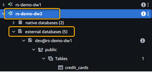
1. Connect to data warehouse 2 as a read-only user and expand the external databases. The following screenshot shows an example using Query Editor V2.
   
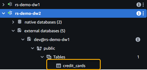
2. Notice the credit_cards table from data warehouse 1 when you expand the catalog.
   
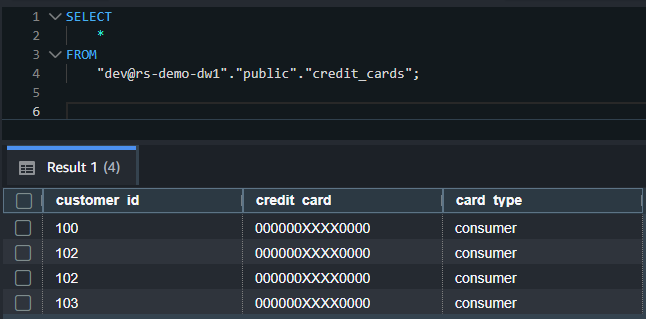
3. Run the following SQL to query the table. Replace rs-demo-dw1 in the following SQL with the catalog name you gave while registering data warehouse 1:

   -- SQL to query credit cards table in data warehouse1. 
   SELECT * FROM "dev@rs-demo-dw1"."public"."credit_cards";

4. You should see only consumer type credit cards with card details masked in the output. The RLS and DDM policies applied in data warehouse 1 on the IAMR:ReadOnly user are enforced even though you queried the table from a different data warehouse.
   The following screenshot shows an example output.
   
5. For auditing, you can run SHOW commands to view the policies applied on the tables for the roles:

   -- Show all RLS policies in the database.
   SHOW RLS POLICIES FROM DATABASE "dev@rs-demo-dw1";
   -- Show all masking policies in the database.
   SHOW MASKING POLICIES FROM DATABASE "dev@rs-demo-dw1";

This example demonstrates the power of federated permissions: security policies defined one time on a warehouse automatically enforce across your warehouses, maintaining compliance without duplicating policy definitions.

Considerations

Keep in mind the following when using federated permissions:

• Amazon Redshift federated permissions are applied for the data warehouses in the same account and Region.
• You can connect to the Redshift data warehouse using IAM users and roles or SSO credentials from your IdP integrated through IAM Identity Center.
• Local users can assume global identities to leverage the federated permissions.
• Amazon Redshift federated permissions are available at no additional cost in Regions where Amazon Redshift is available. You pay only for your existing Amazon Redshift compute and Data Catalog usage.
• Refer Considerations when using Amazon Redshift federated permissions for further details.

Clean up

To avoid incurring future charges, delete the resources you created, including the Redshift data warehouses and IAM roles.

Conclusion

Amazon Redshift federated permissions transform multi-warehouse data governance into a streamlined, automated process. For organizations operating multiple Redshift warehouses, federated permissions deliver immediate value by reducing administrative time and supporting consistent security enforcement. The familiar SQL interface and backward compatibility with existing Redshift permissions enable rapid adoption without requiring teams to learn new governance models.

The integration with IAM and IAM Identity Center provides enterprise-grade identity management with SSO capabilities, and the automatic mounting of registered catalogs simplifies data discovery and cross-warehouse analytics. If you are currently using Amazon Redshift local permissions, refer to the tool described in Modernize Amazon Redshift authentication by migrating user management to AWS IAM Identity Center.

To learn more and get started, see Amazon Redshift Federated Permissions documentation.

About the authors

Post Syndicated from Satesh Sonti original https://aws.amazon.com/blogs/big-data/simplify-online-analytical-processing-olap-queries-in-amazon-redshift-using-new-sql-constructs-such-as-rollup-cube-and-grouping-sets/

Amazon Redshift is a fully managed, petabyte-scale, massively parallel data warehouse that makes it fast, simple, and cost-effective to analyze all your data using standard SQL and your existing business intelligence (BI) tools.

We are continuously investing to make analytics easy with Redshift by simplifying SQL constructs and adding new operators. Now we are adding ROLLUP, CUBE, and GROUPING SETS SQL aggregation extensions to perform multiple aggregate operations in single statement and easily include subtotals, totals, and collections of subtotals in a query.

In this post, we discuss how to use these extensions to simplify your queries in Amazon Redshift.

Solution overview

Online Analytical Processing (OLAP) is an effective tool for today’s data and business analysts. It helps you see your mission-critical metrics at different aggregation levels in a single pane of glass. An analyst can use OLAP aggregations to analyze buying patterns by grouping customers by demographic, geographic, and psychographic data, and then summarizing the data to look for trends. This could include analyzing the frequency of purchases, the time frames between purchases, and the types of items being purchased. Such analysis can provide insight into customer preferences and behavior, which can be used to inform marketing strategies and product development. For example, a data analyst can query the data to display a spreadsheet showing a company’s certain type of products sold in the US in the month of July, compare revenue figures with those for the same products in September, and then see a comparison of other product sales in the US at the same time period.

Traditionally, business analysts and data analysts use a set of SQL UNION queries to achieve the desired level of detail and rollups. However, it can be very time consuming and cumbersome to write and maintain. Furthermore, the level of detail and rollups that can be achieved with this approach is limited, because it requires the user to write multiple queries for each different level of detail and rollup.

Many customers are considering migrating to Amazon Redshift from other data warehouse systems that support OLAP GROUP BY clauses. To make this migration process as seamless as possible, Amazon Redshift now offers support for ROLLUP, CUBE, and GROUPING SETS. This will allow for a smoother migration of OLAP workloads, with minimal rewrites. Ultimately, this will result in a faster and streamlined transition to Amazon Redshift. Business and data analysts can now write a single SQL to do the job of multiple UNION queries.

In the next sections, we use sample supplier balances data from TPC-H dataset as a running example to demonstrate the use of ROLLUP, CUBE, and GROUPING SETS extensions. This dataset consists of supplier account balances across different regions and countries. We demonstrate how to find account balance subtotals and grand totals at each nation level, region level, and a combination of both. All these analytical questions can be answered by a business user by running simple single-line SQL statements. Along with aggregations, this post also demonstrates how the results can be traced back to attributes participated in generating subtotals.

Data preparation

To set up the use case, complete the following steps:

1. On the Amazon Redshift console, in the navigation pane, choose Editor¸ then Query editor v2.

The query editor v2 opens in a new browser tab.

2. Create a supplier sample table and insert sample data:

create table supp_sample (supp_id integer, region_nm char(25), nation_nm char(25), acct_balance numeric(12,2));

INSERT INTO public.supp_sample (supp_id,region_nm,nation_nm,acct_balance)
VALUES
(90470,'AFRICA                   ','KENYA                    ',1745.57),
(99910,'AFRICA                   ','ALGERIA                  ',3659.98),
(26398,'AMERICA                  ','UNITED STATES            ',2575.77),
(43908,'AMERICA                  ','CANADA                   ',1428.27),
(3882,'AMERICA                  ','UNITED STATES            ',7932.67),
(42168,'ASIA                     ','JAPAN                    ',343.34),
(68461,'ASIA                     ','CHINA                    ',2216.11),
(89676,'ASIA                     ','INDIA                    ',4160.75),
(52670,'EUROPE                   ','RUSSIA                   ',2469.40),
(32190,'EUROPE                   ','RUSSIA                   ',1119.55),
(19587,'EUROPE                   ','GERMANY                  ',9904.98),
(1134,'MIDDLE EAST              ','EGYPT                    ',7977.48),
(35213,'MIDDLE EAST              ','EGYPT                    ',737.28),
(36132,'MIDDLE EAST              ','JORDAN                   ',5052.87);

We took a sample from the result of the following query run on TPC-H dataset. You can use the following query and take sample records to try the SQL statement described in this post:

select s_suppkey supp_id, r.r_name region_nm,n.n_name nation_nm, s.s_acctbal acct_balance
from supplier s, nation n, region r
where
s.s_nationkey = n.n_nationkey
and n.n_regionkey = r.r_regionkey

Let’s review the sample data before running the SQLs using GROUPING SETS, ROLLUP, and CUBE extensions.

The supp_sample table consists of supplier account balances from various nations and regions across the world. The following are the attribute definitions:

• supp_id – The unique identifier for each supplier
• region_nm – The region in which the supplier operates
• nation_nm – The nation in which the supplier operates
• acct_balance – The supplier’s outstanding account balance

GROUPING SETS

GROUPING SETS is a SQL aggregation extension to group the query results by one or more columns in a single statement. You can use GROUPING SETS instead of performing multiple SELECT queries with different GROUP BY keys and merge (UNION) their results.

In this section, we show how to find the following:

• Account balances aggregated for each region
• Account balances aggregated for each nation
• Merged results of both aggregations

Run the following SQL statement using GROUPING SETS:

SELECT region_nm, nation_nm, sum(acct_balance) as total_balance
FROM supp_sample
GROUP BY GROUPING SETS (region_nm, nation_nm);

As shown in the following screenshot, the result set includes aggregated account balances by region_nm, followed by nation_nm, and then both results combined in a single output.

ROLLUP

The ROLLUP function generates aggregated results at multiple levels of grouping, starting from the most detailed level and then aggregating up to the next level. It groups data by particular columns and extra rows that represent the subtotals, and assumes a hierarchy among the GROUP BY columns.

In this section, we show how to find the following:

• Account balances for each combination of region_nm and nation_nm
• Rolled-up account balances for each region_nm
• Rolled-up account balances for all regions

Use the following SQL statement using ROLLUP:

SELECT region_nm, nation_nm, sum(acct_balance) as total_balance
FROM supp_sample
GROUP BY ROLLUP (region_nm, nation_nm)
ORDER BY region_nm,nation_nm;

The following result shows rolled-up values starting from each combination of region_nm and nation_nm and rolls up in the hierarchy from nation_nm to region_nm. The rows with a value for region_nm and NULL value for nation_nm represent the subtotals for the region (marked in green). The rows with NULL value for both region_nm and nation_nm has the grand total—the rolled-up account balances for all regions (marked in red).

ROLLUP is structurally equivalent to the following GROUPING SETS query:

SELECT region_nm, nation_nm, sum(acct_balance) as total_balance
FROM supp_sample
GROUP BY GROUPING SETS((region_nm, nation_nm), (region_nm), ())
ORDER BY region_nm,nation_nm;

You can rewrite the preceding ROLLUP query using GROUPING SETS. However, using ROLLUP is a much simpler and readable construct for this use case.

CUBE

CUBE groups data by the provided columns, returning extra subtotal rows representing the totals throughout all levels of grouping columns, in addition to the grouped rows. CUBE returns the same rows as ROLLUP, while adding additional subtotal rows for every combination of grouping column not covered by ROLLUP.

In this section, we show how to find the following:

• Account balance subtotals for each nation_nm
• Account balance subtotals for each region_nm
• Account balance subtotals for each group of region_nm and nation_nm combination
• Overall total account balance for all regions

Run the following SQL statement using CUBE:

SELECT region_nm, nation_nm, sum(acct_balance) as total_balance
FROM supp_sample
WHERE region_nm in ('AFRICA','AMERICA','ASIA') GROUP BY CUBE(region_nm, nation_nm)
ORDER BY region_nm, nation_nm;

In the preceding query, we added a filter to limit results for easy explanation. You can remove this filter in your test to view data for all regions.

In the following result sets, you can see the subtotals at region level (marked in green). These subtotal records are the same records generated by ROLLUP. Additionally, CUBE generated subtotals for each nation_nm (marked in yellow). Finally, you can also see the grand total for all three regions mentioned in the query (marked in red).

CUBE is structurally equivalent to the following GROUPING SETS query:

SELECT region_nm, nation_nm, sum(acct_balance) as total_balance
FROM supp_sample
WHERE region_nm in ('AFRICA','AMERICA','ASIA') -- added the filter to limit results.  You can remove this filter in your test to view data for all regions
GROUP BY GROUPING SETS((region_nm, nation_nm), (region_nm), (nation_nm), ())
ORDER BY region_nm;

You can rewrite the preceding CUBE query using GROUPING SETS. However, using CUBE is a much simpler and readable construct for this use.

NULL values

NULL is a valid value in a column that participates in GROUPING SETS, ROLLUP, and CUBE, and it’s not aggregated with the NULL values added explicitly to the result set to satisfy the schema of returning tuples.

Let’s create an example table orders containing details about items ordered, item descriptions, and quantity of the items:

-- Create example orders table and insert sample records
CREATE TABLE orders(item_no int,description varchar,quantity int);
INSERT INTO orders(item_no,description,quantity)
VALUES
(101,'apples',10),
(102,null,15),
(103,'banana',20);

--View the data
SELECT * FROM orders;

We use the following ROLLUP query to aggregate quantities by item_no and description:

SELECT item_no, description, sum(quantity)
FROM orders
GROUP BY ROLLUP(item_no, description)
ORDER BY 1,2;

In the following result, there are two output rows for item_no 102. The row marked in green is the actual data record in the input, and the row marked in red is the subtotal record added by the ROLLUP function.

This demonstrates that NULL values in input are separate from the NULL values added by SQL aggregate extensions.

Grouping and Grouping_ID functions

GROUPING indicates whether a column in the GROUP BY list is aggregated or not. GROUPING(expr) returns 0 if a tuple is grouped on expr; otherwise it returns 1. GROUPING_ID(expr1, expr2, …, exprN) returns an integer representation of the bitmap that consists of GROUPING(expr1), GROUPING(expr2), …, GROUPING(exprN).

This feature helps us clearly understand the aggregation grain, slice and dice data, and apply filters when business users are performing analysis. Also provides auditability for the generated aggregations.

For example, let’s use the preceding supp_sampe table. The following ROLLUP query utilizes GROUPING and GROUPING_ID functions:

SELECT region_nm,
nation_nm,
sum(acct_balance) as total_balance,
GROUPING(region_nm) as gr,
GROUPING(nation_nm) as gn,
GROUPING_ID(region_nm, nation_nm) as grn
FROM supp_sample
GROUP BY ROLLUP(region_nm, nation_nm)
ORDER BY region_nm;

In the following result set, the rows rolled up at nation_nm have 1 value for gn. This indicates that the total_balance is the aggregated value for all the nation_nm values in the region. The last row has gr value as 1. It indicates that total_balance is an aggregated value at region level including all the nations. The grn is an integer representation of bitmap (11 in binary translated to 3 in integer representation).

Performance assessment

Performance is often a key factor, and we wanted to make sure we’re offering most performant SQL features in Amazon Redshift. We performed benchmarking with the 3 TB TPC-H public dataset on an Amazon Redshift cluster with different sizes (5-node Ra3-4XL, 2-node Ra3-4XL, 2-node-Ra3-XLPLUS). Additionally, we disabled query caching so that query results aren’t cached. This allows us to measure the performance of the database as opposed to its ability to serve results from cache. The results were consistent across multiple runs.

We loaded the supplier, region, and nation files from the 3 TB public dataset and created a view on top of those three tables, as shown in the following code. This query joins the three tables to create a unified record. The joined dataset is used for performance assessment.

create view v_supplier_balances as
select r.r_name region_nm,n.n_name nation_nm, s.s_acctbal acct_balance
from supplier s, nation n, region r
where
s.s_nationkey = n.n_nationkey
and n.n_regionkey = r.r_regionkey;

We ran the following example SELECT queries using GROUPING SETS, CUBE, and ROLLUP, and captured performance metrics in the following tables.
ROLLUP:

SELECT region_nm, nation_nm, sum(acct_balance) as total_balance
FROM v_supplier_balances
GROUP BY ROLLUP (region_nm, nation_nm)
ORDER BY region_nm;

CUBE:

SELECT region_nm, nation_nm, sum(acct_balance) as total_balance
FROM v_supplier_balances
GROUP BY CUBE(region_nm, nation_nm)
ORDER BY region_nm;

GROUPING SETS:

SELECT region_nm, nation_nm, sum(acct_balance) as total_balance
FROM v_supplier_balances
GROUP BY GROUPING SETS(region_nm, nation_nm)
ORDER BY region_nm;

When we ran the same set of queries for ROLLUP and CUBE and ran with UNION ALL, we saw better performance with ROLLUP and CUBE functionality.

Clean up

To clean up your resources, drop the tables and views you created while following along with the example in this post.

Conclusion

In this post, we talked about the new aggregated extensions ROLLUP, CUBE, and GROUPING SETS added to Amazon Redshift. We also discussed general uses cases, implementation examples, and performance results. You can simplify your existing aggregation queries using these new SQL aggregation extensions and use them in future development for building more simplified, readable queries. If you have any feedback or questions, please leave them in the comments section.

About the Authors

Satesh Sonti is a Sr. Analytics Specialist Solutions Architect based out of Atlanta, specialized in building enterprise data platforms, data warehousing, and analytics solutions. He has over 16 years of experience in building data assets and leading complex data platform programs for banking and insurance clients across the globe.

Yanzhu Ji is a Product Manager on the Amazon Redshift team. She worked on the Amazon Redshift team as a Software Engineer before becoming a Product Manager. She has a rich experience of how the customer-facing Amazon Redshift features are built from planning to launching, and always treats customers’ requirements as first priority. In her personal life, Yanzhu likes painting, photography, and playing tennis.

Dinesh Kumar is a Database Engineer with more than a decade of experience working in the databases, data warehousing, and analytics space. Outside of work, he enjoys trying different cuisines and spending time with his family and friends.