Post Syndicated from Neeraj Kaushik original https://aws.amazon.com/blogs/architecture/modernization-of-real-time-payment-orchestration-on-aws/
The global real-time payments market is experiencing significant growth. According to Fortune Business Insights, the market was valued at USD 24.91 billion in 2024 and is projected to grow to USD 284.49 billion by 2032, with a CAGR of 35.4%. Similarly, Grand View Research reports that the global mobile payment market, valued at USD 88.50 billion in 2024, is expected to grow at a CAGR of 38.0% from 2025 to 2030. (Disclaimer: Third-party market research and statistics are provided for informational purposed only. AWS and IBM make no representations about the accuracy of this information.)
This rapid expansion underscores the urgency for financial institutions to modernize their payment processing infrastructure. Financial institutions often need to process high volume of transactions with near-zero latency to meet stringent service level agreements (SLAs) to support surging mobile payments volume.
However, traditional payment orchestration systems, often built on monolithic architectures, struggle to meet these demands due to latency, availability, and scalability challenges. Additionally, their reliance on on-premises infrastructure leads to higher costs and an impediment to innovation, reinforcing the need for modernization.
As sustainability becomes a priority, organizations are turning to cloud-based solutions to optimize infrastructure, reduce carbon footprints, and enhance energy efficiency. This shift provides scalability and performance, and aligns with global sustainability goals, securing the future of real-time payments.
In this post, we discuss the real-time payment orchestration framework. It uses an event-driven architecture and AWS serverless services to enhance the resiliency, efficiency, and scalability of real-time payments. By decomposing payment processing into distinct business capabilities, financial institutions can improve modularity and flexibility. Implementing tenant-based segregation helps with data isolation and security. Additionally, adopting asynchronous communication through Amazon Managed Streaming for Apache Kafka (Amazon MSK) enhances scalability and resilience.
Traditional real-time payment orchestration
Payment orchestration serves as a middleware solution, streamlining transaction processing across multiple payment methods, gateways, and financial institutions. It orchestrates key business functions such as payment authorization, payment processing, settlement and clearing, compliance and risk management, and account management for both inbound and outbound payment flows.
The following diagram depicts the high-level business capabilities supported by payment orchestrators across various payment flows, including real-time payments, digital disbursements, tax payments, wires, and more.
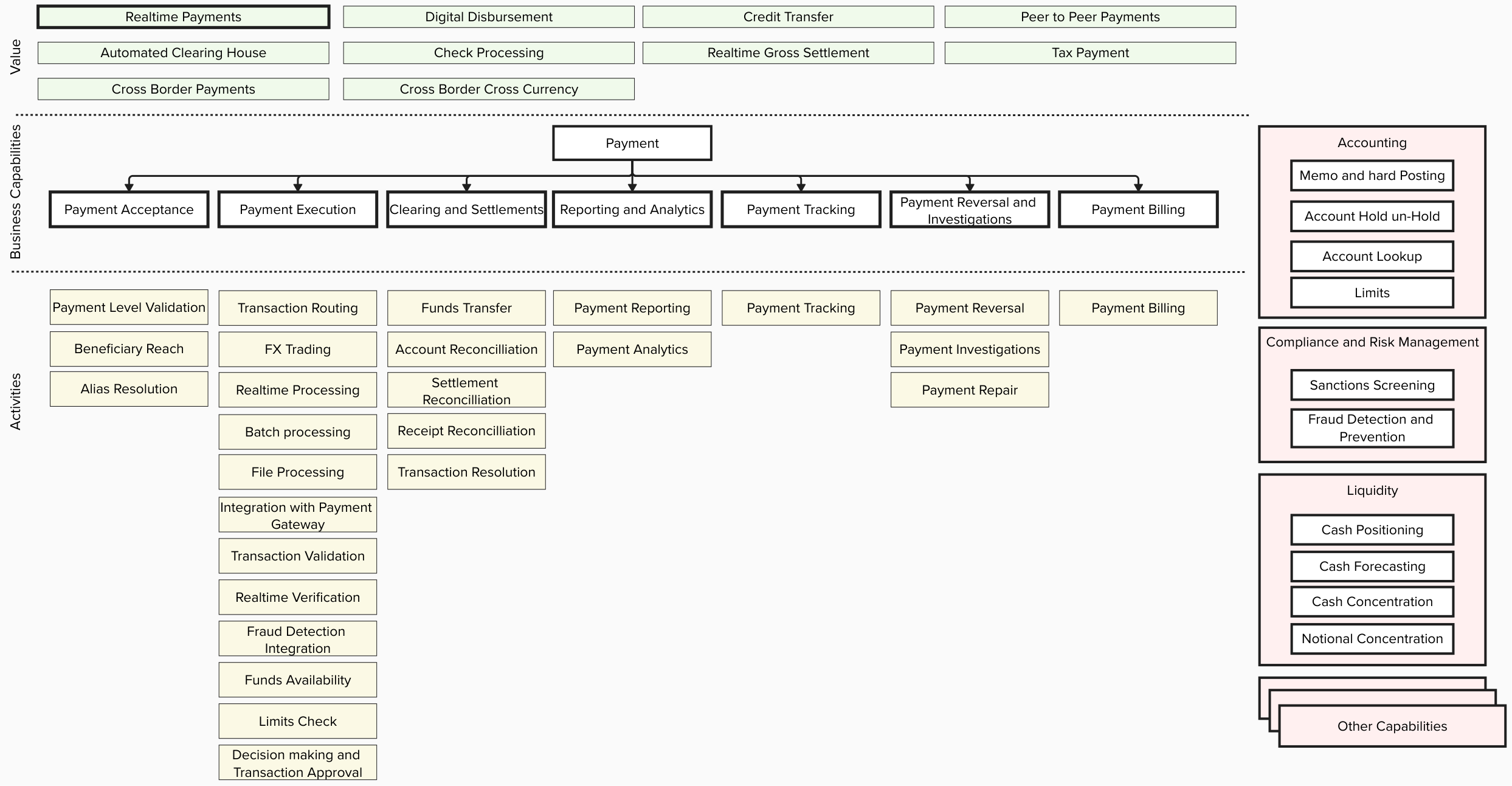
Detailed flowchart depicting a payment processing system with multiple components. The diagram shows primary payment types at the top (including Realtime Payments, Digital Disbursement, Credit Transfer, and Peer to Peer Payments) flowing down through core processing stages including Payment Acceptance, Execution, Clearing, Reporting, Tracking, Reversals, and Billing.
Many financial institutions adopt a tenant-based approach organized by geography due to varying clearing processes, localized regulations, and transaction requirements across AWS Regions. However, without proper separation of services, teams often continue to add region-specific logic to existing services, gradually increasing their monolithic complexity and using the same infrastructure for all payment flows.
Traditional payment systems process transactions linearly, with each step waiting for the previous one to complete. However, analysis of payment workflows reveals numerous opportunities for parallel execution:
- Sanctions screening and fraud detection – Compliance and fraud checks can run simultaneously with initial routing decisions, rather than sequentially blocking all subsequent processing
- Payment routing and authorization requests – When basic validations are complete, routing and authorization can proceed in parallel rather than one after another
- Payment execution and ledger updates – The actual payment execution doesn’t need to wait for ledger records to be updated—these can occur concurrently
- Settlement, reconciliation, and tracking – These post-transaction processes can be initiated independently as soon as the primary transaction is complete
This parallel approach can dramatically improve throughput and reduce latency compared to traditional queue-based systems where operations form a sequential chain that extends processing time and creates bottlenecks.
Most legacy payment orchestration systems rely heavily on on-premises virtual machines (VMs), leading to several challenges:
- Multi-Region support for disaster recovery and multi-tenancy resulting in significant capital expenditure and operational overhead
- High latency and SLA issues caused by sequential message processing and delays between globally separated data centers
- Limited reusability of payment flows as monolithic architectures require region-specific changes for local clearing mechanisms and regulations, increasing complexity and costs
- Scalability challenges and high memory consumption due to inefficient resource utilization and execution of irrelevant logic across regions
- Complex cross-border payment routing caused by variations in clearing rules, transaction limits, and local regulations, increasing latency and routing errors
- Integration challenges with diverse data formats because legacy systems rely on proprietary standards (for example, ISO 20022, SWIFT MT), complicating data conversion and compliance
- High deployment complexity for new payment flows due to monolithic architectures requiring extensive region-specific modifications, slowing time to market
- Environmental impact and high carbon footprint from on-premises infrastructure consuming excessive energy, whereas cloud-based approaches improve efficiency
Solution overview
To overcome these challenges, the proposed architecture embraces the following design principles to build a future-ready, real-time payment orchestration solution:
- Performance at scale – Handling over 1,000 transactions per second (TPS) with consistent low latency under varying load conditions.
- High availability – Achieving 99.999% uptime to meet the strict requirements of financial transactions.
- Geographic resilience – Supporting global operations with region-specific compliance while maintaining consistent performance.
- Cost optimization – Reducing total cost of ownership through efficient resource utilization and serverless technologies.
- Security and compliance – Supporting data protection and regulatory adherence across different jurisdictions.
- Operational simplicity – Streamlining deployment, monitoring, and maintenance across the payment ecosystem.
- Microservices – Decomposing payment processing into distinct business capabilities, so financial institutions can improve modularity and flexibility. This microservices-based approach allows for independent scaling and development of critical components.
The following diagram depicts the high-level solution architecture for real-time payments. The existing channels using synchronous or asynchronous APIs can be modified to use edge-optimized endpoints to reduce latency.
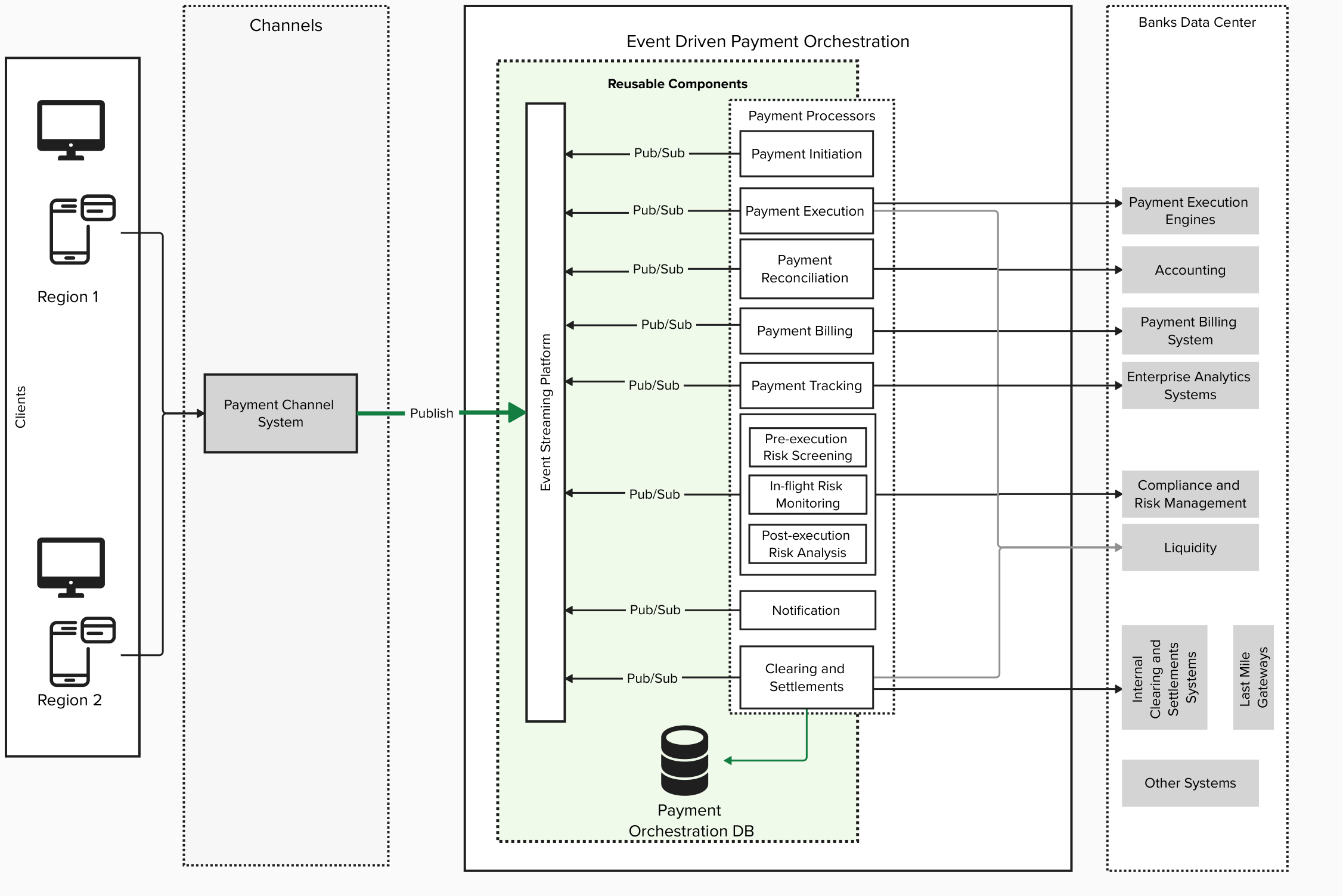
Architecture diagram detailing an AWS-based payment orchestration platform utilizing event-driven principles. Features reusable components across two regions, with dedicated modules for payment initiation, execution, reconciliation, billing, and risk management. Implements pub/sub messaging patterns for inter-component communication and connects to enterprise systems including accounting, compliance, and analytics.
An event-driven architecture is used for payment orchestration, which handles communication through a pub/sub pattern. This architecture maintains persistent connections, improving performance of the end-to-end real-time payment processing.
The event-driven architecture for real-time payment processing allows multiple payment operations to occur simultaneously using different adaptors, as opposed to the traditional systems where payment processes are sequential and flow through a single pipeline. Payment events are distributed to specialized payment processor microservices based on their function (initiation, execution, tracking, settlements), enabling each to process independently without waiting for others to complete.
Because we’re transitioning from sequential processing to distributed, maintaining transaction traceability is crucial. The payment tracking adapters shown in the preceding diagram connect to enterprise analytics systems, creating a specialized layer for monitoring transactions. The pub/sub model allows for attaching correlation IDs to events, enabling systems to track related events across different topics and processing stages.
A standardized event schema serves as the foundation for this architecture, providing consistency across regional deployments while allowing for customization at the adapter level. This schema defines uniform event structures containing tenant-specific metadata and supports versioning to accommodate evolving requirements. By isolating region-specific variations to the adapter layer, the solution maintains core functionality while interfacing with diverse enterprise systems through configuration-driven customization rather than code changes.
For most payment processes, especially those with independent processing steps that can run in parallel, this architecture delivers net performance gains despite the topic switching overhead, particularly for complex transactions where multiple independent validations or processing steps are required.
Deployment on the AWS Cloud
The solution uses edge-optimized Amazon API Gateway for channels. An edge-optimized API endpoint routes requests to the nearest Amazon CloudFront Point of Presence (POP), which can help in cases where your clients are geographically distributed to enable efficient routing within each geographical region, enhancing global responsiveness by minimizing network round trips and making sure requests take the shortest possible path before transitioning from the public internet to the client network.
The following diagram illustrates the high-level solution architecture for real-time payments.

Comprehensive AWS payment orchestration solution implementing modern cloud-native architecture principles. Core processing logic implemented as Lambda functions covering initiation, execution, reconciliation, billing, tracking, risk management, and settlement workflows. Leverages Amazon MSK for reliable event streaming between components, with dedicated Kafka topics for each processing stage. Data persistence handled by Amazon DynamoDB, supporting cross-region operations. Architecture demonstrates AWS best practices for financial services, including regional redundancy, serverless computing, managed services, and event-driven design patterns. System integrates with external banking infrastructure and enterprise systems while maintaining separation of concerns through microservices architecture. Features built-in support for compliance monitoring, risk management, and payment tracking through specialized Lambda functions.
The solution uses Amazon MSK to implement an event-driven architecture that efficiently handles both inbound and outbound channels traffic through API requests and asynchronous message-based events. Amazon MSK communicates using a high-performance binary protocol between producers, consumers, and brokers, providing low latency and high throughput. Real-time payments are logically partitioned across multiple tenants within geographical regions—North America, EMEA, LATAM, and Asia-Pacific.
Each real-time payment tenant follows an active/active disaster recovery strategy by deploying MSK clusters across multiple AWS Regions, designed to achieve high availability and resilience. Amazon MSK offer both serverless and provisioned cluster options. The team can decide to select one or the other depending on the non-functional requirements and team expertise. Amazon MSK automatically manages partition leadership with leaders in primary Regions and followers in secondary Regions. During failover, leaders are re-elected in healthy Regions, designed to help maintain processing capabilities during regional incidents. Sticky partitioning uses consistent hashing for deterministic routing, and cooperative rebalancing enables efficient failover. Multi-AZ deployment provides zone redundancy and isolated clusters per Region for data sovereignty compliance through programmatic AWS Identity and Access Management (IAM) and virtual private cloud (VPC) boundaries.
To support seamless cross-Region replication and maintain message continuity, Amazon MSK Replicator—a fully managed feature of Amazon MSK—is used to replicate topics and synchronize consumer group offsets across clusters. MSK Replicator simplifies the process of building multi-Region Kafka applications by not needing custom code, open-source tool configuration, or infrastructure management. It automatically provisions and scales the necessary resources, so teams can focus on business logic while only paying for the data being replicated. In the event of a regional outage or failover, traffic can be automatically redirected to a healthy Region without data loss or service disruption, providing near-zero Recovery Time Objectives (RTOs) and uninterrupted operations for downstream services such as payment processors and audit trail consumers.
In addition to regional redundancy, the architecture uses an event-driven architecture to enable parallel and decoupled processing of payment transactions. Events such as transaction initiation, validation, and settlement are emitted asynchronously and consumed by various microservices independently, which drastically reduces end-to-end latency.
To process these events at scale, the architecture can use AWS Lambda, Amazon Elastic Container Service (Amazon ECS), or Amazon Elastic Kubernetes Service (Amazon EKS) depending upon non-functional requirements. Automatic scaling responds to Amazon CloudWatch metrics, and exponential backoff retry logic with dead-letter queues (DLQs) handles throttling scenarios. Circuit breakers prevent cascade failures during high error rates.
One of the key benefits of the solution is the reusability of payment flows across different regions. Although each region has its own unique compliance requirements and settlement rules, the core functionalities of real-time payments (payment authorization, payment processing, settlement and clearing) are largely similar. This reusability enables rapid deployment of payment solutions across new regions without rearchitecting the entire system. For example, the real-time payment system in the US and UK might share similar business logic for real-time gross settlement but differ in the clearing and compliance requirements. The solution treats these as bounded contexts within the microservices architecture, providing flexibility while making sure each region can handle its own specific rules and regulations.
Sustainability
AWS relentlessly innovates its infrastructure design, build, and operations to make progress towards net-zero carbon by 2040 and being water positive by 2030. Amazon MSK with AWS Graviton based instances use up to 60% less energy than comparable M5 instances, helping you achieve your sustainability goals. Lambda is inherently sustainable by design. Its serverless model makes sure compute resources are only used when needed, drastically reducing idle infrastructure and wasted energy. Instead of keeping always-on servers for infrequent tasks, Lambda provisions compute power just-in-time, achieving near-zero idle capacity.
Security and compliance in financial services
Given the sensitive nature of payment transactions and financial data, you should apply the security controls required to meet financial regulations such as AWS PCI DSS and AWS Federal Information Processing Standard (FIPS) 140-3 according to your organization’s needs.
The solution should incorporate multi-layered security controls, continuous monitoring, and automated compliance auditing to meet the rigorous expectations of banking regulators and internal risk teams. For more information, refer to Security Guidance.
Conclusion
The modernization of payment orchestration systems using an event-driven architecture and AWS serverless technologies marks a significant advancement in meeting the demands of today’s rapidly evolving financial services landscape. This solution addresses the key challenges faced by traditional payment systems while delivering substantial benefits in performance, scalability, cost optimization, global resilience, sustainability, and compliance. By using cutting-edge cloud technologies and robust security controls, financial institutions can now build a future-ready foundation that adapts to evolving business needs while maintaining the highest standards of performance, security, and reliability. As the real-time payments market continues its explosive growth, this modern architecture provides a solution that meets today’s demands and is also well-positioned to support tomorrow’s payment innovations. Organizations looking to modernize their payment infrastructure can use this blueprint to accelerate their digital transformation journey, supporting sustainable, secure, and efficient payment processing at scale in an increasingly competitive global marketplace.
The architecture presented here is for reference purposes only. IBM will work closely with you to deploy the solution in accordance with industry standards and compliance requirements.For additional resources, refer to:
- IBM Consulting on AWS
- AWS for Financial Services
- Transforming transactions: Streamlining PCI compliance using AWS serverless architecture
- Best practices for right-sizing your Apache Kafka clusters to optimize performance and cost
- How to choose the right Amazon MSK cluster type for you
- AWS Shared Responsibility Model
- AWS Federal Information Processing Standard (FIPS) 140-3
- Sustainability with AWS Graviton
- AWS PCI DSS
IBM Consulting is an AWS Premier Tier Services Partner that helps customers who use AWS to harness the power of innovation and drive their business transformation. They are recognized as a Global Systems Integrator (GSI) for over 22 competencies, including Financial Services Consulting. For additional information, please contact an IBM Representative.


 Amit Maindola is a Senior Data Architect focused on data engineering, analytics, and AI/ML at Amazon Web Services. He helps customers in their digital transformation journey and enables them to build highly scalable, robust, and secure cloud-based analytical solutions on AWS to gain timely insights and make critical business decisions.
 Arghya Banerjee is a Sr. Solutions Architect at AWS in the San Francisco Bay Area, focused on helping customers adopt and use the AWS Cloud. He is focused on big data, data lakes, streaming and batch analytics services, and generative AI technologies.
 Melody Yang is a Principal Analytics Architect for Amazon EMR at AWS. She is an experienced analytics leader working with AWS customers to provide best practice guidance and technical advice in order to assist their success in data transformation. Her areas of interests are open-source frameworks and automation, data engineering and DataOps.
 Gaurav Parekh is a Solutions Architect at AWS, specializing in generative AI and data analytics, with extensive experience building production AI systems on AWS.


 Guy Bachar is a Senior Solutions Architect at AWS based in New York. He specializes in assisting capital markets customers with their cloud transformation journeys. His expertise encompasses identity management, security, and unified communication.
 Sercan Karaoglu is Senior Solutions Architect, specialized in capital markets. He is a former data engineer and passionate about quantitative investment research.
 Boris Litvin is a Principal Solutions Architect at AWS. His job is in financial services industry innovation. Boris joined AWS from the industry, most recently Goldman Sachs, where he held a variety of quantitative roles across equity, FX, and interest rates, and was CEO and Founder of a quantitative trading FinTech startup.
 Salim Tutuncu is a Senior Partner Solutions Architect Specialist on Data & AI, based in Dubai with a focus on the EMEA. With a background in the technology sector that spans roles as a data engineer, data scientist, and machine learning engineer, Salim has built a formidable expertise in navigating the complex landscape of data and artificial intelligence. His current role involves working closely with partners to develop long-term, profitable businesses using the AWS platform, particularly in data and AI use cases.
 Alex Tarasov is a Senior Solutions Architect working with Fintech startup customers, helping them to design and run their data workloads on AWS. He is a former data engineer and is passionate about all things data and machine learning.
 Jiwan Panjiker is a Solutions Architect at Amazon Web Services, based in the Greater New York City area. He works with AWS enterprise customers, helping them in their cloud journey to solve complex business problems by making effective use of AWS services. Outside of work, he likes spending time with his friends and family, going for long drives, and exploring local cuisine.


 Julien Lafaye is a director at Capital Fund Management (CFM) where he is leading the implementation of a data platform on AWS. He is also heading a team of data scientists and software engineers in charge of delivering intraday features to feed CFM trading strategies. Before that, he was developing low latency solutions for transforming & disseminating financial market data. He holds a Phd in computer science and graduated from Ecole Polytechnique Paris. During his spare time, he enjoys cycling, running and tinkering with electronic gadgets and computers.
 Matthieu Bonville is a Solutions Architect in AWS France working with Financial Services Industry (FSI) customers. He leverages his technical expertise and knowledge of the FSI domain to help customer architect effective technology solutions that address their business challenges.
 Joel Farvault is Principal Specialist SA Analytics for AWS with 25 years’ experience working on enterprise architecture, data governance and analytics, mainly in the financial services industry. Joel has led data transformation projects on fraud analytics, claims automation, and Master Data Management. He leverages his experience to advise customers on their data strategy and technology foundations.


 apc-crr
 Deployment time: 307.88s
Stack ARN:
arn:aws:cloudformation:<aws_region>:<aws_account>:stack/apc-crr/<stack_id>
Deployment time: 307.88s
Stack ARN:
arn:aws:cloudformation:<aws_region>:<aws_account>:stack/apc-crr/<stack_id>


 Clarisa Tavolieri is a Software Engineering graduate with qualifications in Business, Audit, and Strategy Consulting. With an extensive career in the financial and tech industries, she specializes in data management and has been involved in initiatives ranging from reporting to data architecture. She currently serves as the Global Head of Cyber Data Management at Zurich Group. In her role, she leads the data strategy to support the protection of company assets and implements advanced analytics to enhance and monitor cybersecurity tools.
 Austin Rappeport is a Computer Engineer who graduated from the University of Illinois Urbana/Champaign in 2011 with a focus in Computer Security. After graduation, he worked for the Federal Energy Regulatory Commission in the Office of Electric Reliability, working with the North American Electric Reliability Corporation’s Critical Infrastructure Protection Standards on both the audit and enforcement side, as well as standards development. Austin currently works for Zurich Insurance as the Global Head of Detection Engineering and Automation, where he leads the team responsible for using Zurich’s security tools to detect suspicious and malicious activity and improve internal processes through automation.
 Samantha Gignac is a Global Security Architect at Zurich Insurance. She graduated from Ferris State University in 2014 with a Bachelor’s degree in Computer Systems & Network Engineering. With experience in the insurance, healthcare, and supply chain industries, she has held roles such as Storage Engineer, Risk Management Engineer, Vulnerability Management Engineer, and SOC Engineer. As a Cybersecurity Architect, she designs and implements secure network systems to protect organizational data and infrastructure from cyber threats.
 Claire Sheridan is a Principal Solutions Architect with Amazon Web Services working with global financial services customers. She holds a PhD in Informatics and has more than 15 years of industry experience in tech. She loves traveling and visiting art galleries.
 Jake Obi is a Principal Security Consultant with Amazon Web Services based in South Carolina, US, with over 20 years’ experience in information technology. He helps financial services customers improve their security posture in the cloud. Prior to joining Amazon, Jake was an Information Assurance Manager for the US Navy, where he worked on a large satellite communications program as well as hosting government websites using the public cloud.
 Srikanth Daggumalli is an Analytics Specialist Solutions Architect in AWS. Out of 18 years of experience, he has over a decade of experience in architecting cost-effective, performant, and secure enterprise applications that improve customer reachability and experience, using big data, AI/ML, cloud, and security technologies. He has built high-performing data platforms for major financial institutions, enabling improved customer reach and exceptional experiences. He is specialized in services like cross-border transactions and architecting robust analytics platforms.
 Freddy Kasprzykowski is a Senior Security Consultant with Amazon Web Services based in Florida, US, with over 20 years’ experience in information technology. He helps customers adopt AWS services securely according to industry best practices, standards, and compliance regulations. He is a member of the Customer Incident Response Team (CIRT), helping customers during security events, a seasoned speaker at AWS re:Invent and AWS re:Inforce conferences, and a contributor to open source projects related to AWS security.


 Toney Thomas is a Data Architect and Data Engineering Lead at Bluestone, renowned for his role in envisioning and coining the company’s pioneering data strategy. With a strategic focus on harnessing the power of advanced technology to tackle intricate business challenges, Toney leads a dynamic team of Data Engineers, Reporting Engineers, Quality Assurance specialists, and Business Analysts at Bluestone. His leadership extends to driving the implementation of robust data governance frameworks across diverse organizational units. Under his guidance, Bluestone has achieved remarkable success, including the deployment of innovative platforms such as a fully governed data mesh business data system with embedded data quality mechanisms, aligning seamlessly with the organization’s commitment to data democratization and excellence.
 Ben Vengerovsky is a Data Platform Product Manager at Bluestone. He is passionate about using cloud technology to revolutionize the company’s data infrastructure. With a background in mortgage lending and a deep understanding of AWS services, Ben specializes in designing scalable and efficient data solutions that drive business growth and enhance customer experiences. He thrives on collaborating with cross-functional teams to translate business requirements into innovative technical solutions that empower data-driven decision-making.
 Rada Stanic is a Chief Technologist at Amazon Web Services, where she helps ANZ customers across different segments solve their business problems using AWS Cloud technologies. Her special areas of interest are data analytics, machine learning/AI, and application modernization.