All posts by Shailaja Suresh

Field Notes: Building an Industrial Data Platform to Gather Insights from Operational Data

Post Syndicated from Shailaja Suresh original https://aws.amazon.com/blogs/architecture/field-notes-building-an-industrial-data-platform-to-gather-insights-from-operational-data/

Co-authored with Russell de Pina, former Sr. Partner Solutions Architect at AWS

Manufacturers looking to achieve greater operational efficiency need actionable insights from their operational data. Traditionally, operational technology (OT) and enterprise information technology (IT) existed in silos with various manual processes to clean and process data. Leveraging insights at a process level requires converging data across silos and abstracting the right data for the right use case in a scalable fashion.

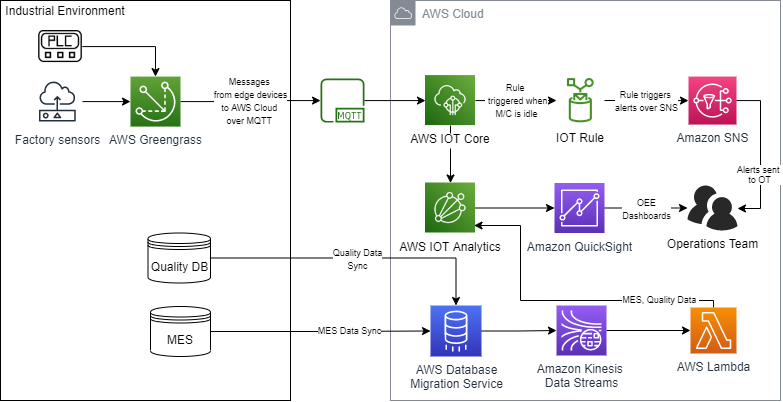
The AWS Industrial Data Platform (IDP) facilitates the convergence of enterprise and operational data for gathering insights that lead to overall operational efficiency of the plant. In this blog, we demonstrate a sample AWS IDP architecture along with the steps to gather data across multiple data sources on the shop floor.

Overview of solution

With the IDP Reference Architecture as the backdrop, let us walk through the steps to implement this solution. Let us say we have gas compressors being used in our factory. The Operations Team has identified an anomaly in the wear of the bearings used in some of these compressors. Currently the bearings are supplied by two manufacturers, ABC and XYZ.

The graphs in Figures 1 and 2 show the expected and actual performance data of the bearings with respect to the vibration (actual and expected) against time. The points represent a cluster of plots which are represented as single dots here. The Mean Time Between Maintenance (MTBM) per the manufacturer for these bearings is five years. The factory has detected that for ABC bearings, the actual vibrations detected during its half-life is much more than the normal (expected) as shown. This clearly requires further analysis to identify the root cause for this discrepancy to prevent compressor breakdowns, unplanned downtime and cost.

ABC Bearings Anomoly

Figure 1 – ABC Bearings Anomaly

XYZ Bearings Vibration

Figure 2 – XYZ Bearings Vibration

Although the deviation observed from expected is much less in XYZ bearings, there is still a deviation which needs to be understood. This blog provides an overview of how the various AWS services of the IDP architecture help with this analysis. Figure 3, shows the AWS architecture used for this specific use case.

IDP AWS Architecture to solve for the Bearings Anomaly 

Figure 3 – IDP AWS Architecture to solve for the Bearings Anomaly

Tracking Anomaly Data

The sensors on the compressor bearings send the vibration/chatter data to AWS through AWS IoT core. Amazon Lookout for Equipment is configured as detailed out in the user guide with the necessary data formatting guidelines.

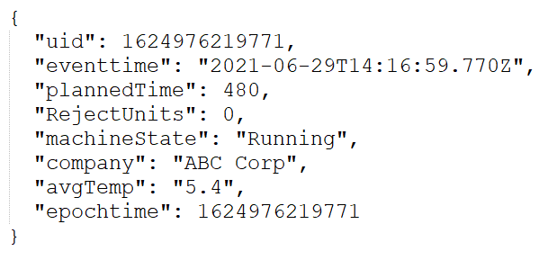
The raw sensor data from IoT Core which is in a JSON format is converted into a CSV format with the necessary headers to match the schema (one schema for each sensor) in Figure 7 using AWS Lambda. This CSV conversion is needed for the data to be processed by Amazon Lookout for Equipment. A sample sensor data from the ABC sensor, the AWS Lambda code snippet to convert this JSON to CSV and the output CSV which is to be ingested into Lookout for Equipment are shown in Figure 4,5 and 6 respectively. For detailed steps on how a dataset is created to be ingested into Lookout For Equipment, please refer the user guide.

Figure 4: Sample Sensor Data from ABC Bearings’ Sensor

Figure 4: Sample Sensor Data from ABC Bearings’ Sensor

import boto3
import botocore
import csv
import json

def lambda_handler(event, context):
    BUCKET_NAME = 'L4EData' 
    OUTPUT_KEY = 'csv/ABCSensor.csv' # OUTPUT FILE 
    INPUT_KEY = 'ABCSensor.json'# INPUT FILE 
    s3client = boto3.client('s3')
    s3 = boto3.resource('s3') 
    
    obj = s3.Object(BUCKET_NAME, INPUT_KEY)
    data = obj.get()['Body'].read().decode('utf-8')
    json_data = json.loads(data)
    print(json_data)

    
    output_file_path = "/tmp/data.csv"
    
    with open(output_file_path, "w") as file:
        csv_file = csv.writer(file)
        csv_file.writerow(['TIMESTAMP', 'Sensor'])
        for item in json_data:
            csv_file.writerow([item.get('TIMESTAMP'),item.get('Sensor')])
    
    csv_binary = open(output_file_path, 'rb').read()
    
    
    try:
        obj = s3.Object(BUCKET_NAME, OUTPUT_KEY)
        obj.put(Body=csv_binary)
    except botocore.exceptions.ClientError as e:
        if e.response['Error']['Code'] == "404":
            print("The object does not exist.")
        else:
            raise
    
    try:
        download_url = s3client.generate_presigned_url(
                         'get_object',
                          Params={
                              'Bucket': BUCKET_NAME,
                              'Key': OUTPUT_KEY
                              },
                          ExpiresIn=3600
        )
        return json.dumps(download_url)
    except Exception as e:
        raise utils_exception.ErrorResponse(400, e, Log)

Figure 5 –  AWS Lambda Python Code snippet to Convert CSV to JSON

Figure 6: Output CSV from AWS Lambda with Timestamp and Vibration values from Sensor

Figure 6 – Output CSV from AWS Lambda with Timestamp and Vibration values from Sensor

Figure 7: Data Schema used for Dataset Ingestion in Amazon Lookout for Equipment for ABC Vibration Sensor

Figure 7 – Data Schema used for Dataset Ingestion in Amazon Lookout for Equipment for ABC Vibration Sensor

Once the model is trained the anomaly is detected on bearing ABC as already stated.

Analyze Factory Environment Data

For our analysis, it is important to factor in the factory environment conditions. There are variables like factory humidity, machine temperature, bearing lubrication levels that could attribute to increased vibration. We have all the environment data gathered from factory sensors made available through AWS IoT Core as shown in Figure 3. Since the number of parameters measured through the factory sensors can change over time, the architecture uses a no-SQL database, Amazon DynamoDB, to persist this data for downstream analysis.

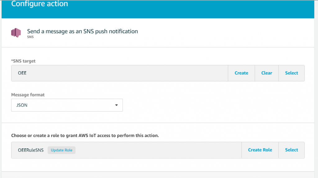
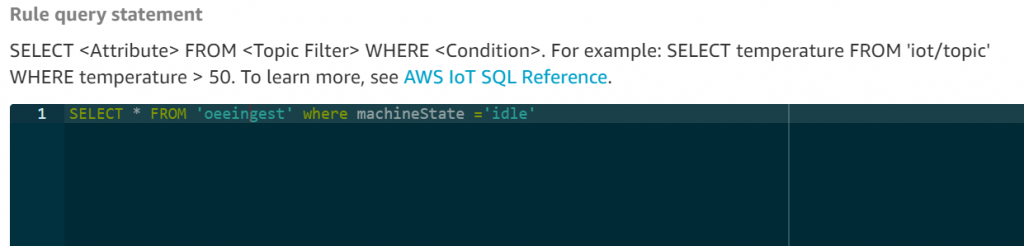
Since we only need sensor events that exceed a particular threshold, we set rules under AWS IoT Core to capture those events that could potentially cause increased vibration on the bearings. For example, we just want only those events that exceed a temperature threshold, say anything above 75-degree Fahrenheit along with the timestamp in Amazon DynamoDB. This is beyond the normal operating temperature for the bearings and certainly demands our interest.

So, we set a rule trigger as shown in Figure 8 in the Rule query statement while defining an action under IoT Core. The flow of events from an IoT sensor to Amazon DynamoDB is illustrated in Figure 9.

Figure 8 - Define a Rule in IoT Core

Figure 8 – Define a Rule in IoT Core

The events are received on a minute basis. So, if there are 3 records inserted in Amazon DynamoDB on a day, it means that there has been a temperature threshold breach for a maximum of 3 minutes.

We set up similar rules and actions to DynamoDB for humidity and compressor lubrication levels.

Figure 9: Event from IoT factory sensor to Amazon DynamoDB

Figure 9: Event from IoT factory sensor to Amazon DynamoDB

1)      Factory Data Storage

It is required to factor in both the factory data like machine id, shift number, shop floor and the operator data like the operator name, machine-operator relationships, operator’s shift, etc., for this analysis since we are drilling down to the granular details of which operators where working on the machines which have ABC bearings. Since this data is relational, it is stored in Amazon Aurora. We opt for the serverless option of the Aurora database since the operations team requires a database that is fully managed.

The  data of the vendors who supply ABC and XYZ bearings and their contracts  are stored in Amazon S3. We also have the operators’ performance scores pre-calculated and stored in Amazon S3.

2)      Querying the Data Lake

Now that we have data ingested and stored in various channels – Amazon S3, AWS IoT Core, Amazon DynamoDB and Amazon Aurora, it is required that we collate this data for further analysis and querying. We use Athena Federated Query  under Amazon Athena for querying across these multiple data sources and store the results in Amazon S3 as shown in Figure 10. It is required that we create a workgroup and configure connectors to set up Amazon S3, Amazon DynamoDB and Amazon Aurora as the data sources under Amazon Athena. The detailed steps to create and connect the data sources are provided in the user guide.

Figure 10: Athena Federated Query across Data Sources

Figure 10: Athena Federated Query across Data Sources

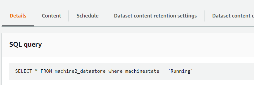
We are now interested to gather some insights across the three different data sources. Let us find all those machines and their corresponding operators with performance scores in factory shop floor 1 which have the lubrication levels as demonstrated in Figure 11.

Figure 11: Query to Determine Operators and their Performance

Figure 11: Query to Determine Operators and their Performance

From the output in Table 1, we see that operators on these machines which have the machine temperature levels of above the threshold to be having good scores (above 5, which is the average) based on past performance. Hence, we could conclude for now that they have been operating these machines under the normal expected conditions with the right controls and settings.

Table 1: Operators and their Scores

Table 1: Operators and their Scores

We would then want to find all those machines which have ABC Bearings and the vendors who supplied them as demonstrated in Figure 12.

Figure 12: Vendors Supplying ABC Bearings

Figure 12: Vendors Supplying ABC Bearings

Table 2: Names of Vendors Who Supply ABC Bearings

Table 2: Names of Vendors Who Supply ABC Bearings

As a next step, we would want to reach out to the vendors, Jane Doe Enterprises and Scott Inc.(see Table 2) to report the issue with ABC Bearings. The next step is to potentially modify the supply contracts and purchase only from XYZ manufacturer and/or to look for other bearing manufacturers in the vendor supply chain.

Conclusion

In this blog, we covered a sample use case to demonstrate how the AWS Industrial Data Platform can help gather actionable insights from factory floor data to gain operation efficiencies. We also did a walkthrough of a sample use case to demonstrate how the various AWS services can be used to build a scalable data platform for seamless querying and processing of data coming in with various formats.

Field Notes: Tracking Overall Equipment Effectiveness with AWS IoT Analytics and Amazon QuickSight

Post Syndicated from Shailaja Suresh original https://aws.amazon.com/blogs/architecture/field-notes-tracking-overall-equipment-effectiveness-with-aws-iot-analytics-and-amazon-quicksight/

This post was co-written with Michael Brown, Senior Solutions Architect, Manufacturing at AWS.

Overall equipment effectiveness (OEE) is a measure of how well a manufacturing operation is utilized (facilities, time and material) compared to its full potential, during the periods when it is scheduled to run. Measuring OEE provides a way to obtain actionable insights into manufacturing processes to increase the overall productivity along with reduction in waste.

In order to drive process efficiencies and optimize costs, manufacturing organizations need a scalable approach to accessing data across disparate silos across their organization. In this blog post, we will demonstrate how OEE can be calculated, monitored, and scaled out using two key services: AWS IoT Analytics and Amazon QuickSight.

Overview of solution

We will use the standard OEE formulas for this example:

Table 1. OEE Calculations
Availability = Actual Time / Planned Time (in minutes)
Performance = (Total Units/Actual Time) / Ideal Run Rate
Quality = Good Units Produced / Total Units Produced
OEE = Availability * Performance * Quality

To calculate OEE, identify the following data for the calculation and its source:

Table 2. Source of supporting data
Supporting Data Method of Ingest
Total Planned Scheduled Production Time Manufacturing Execution Systems (MES)
Ideal Production Rate of Machine in Units MES
Total Production for the Scheduled time Programmable Logic Controller (PLC), MES
Total Number of Off-Quality units produced PLC, Quality DB
Total Unplanned Downtime in minutes PLC

For the purpose of this exercise, we assume that the supporting data is ingested as an MQTT message.

As indicated in Figure 1, the data is ingested into AWS IoT Core and then sent to AWS IoT Analytics by an IoT rule to calculate the OEE metrics. These IoT data insights can then be viewed from a QuickSight dashboard. Specific machine states, like machine idling, could be notified to the technicians through email or SMS by Amazon Simple Notification Service (Amazon SNS). All OEE metrics can then be republished to AWS IoT Core so any other processes can consume them.

Figure 1. Tracking OEE using PLCs with AWS IoT Analytics and QuickSight

Walkthrough

The components of this solution are:

  • PLC – An industrial computer that has been ruggedized and adapted for the control of manufacturing processes, such as assembly lines, robotic devices, or any activity that requires high reliability, ease of programming, and process fault diagnosis.
  • AWS IoT Greengrass – Provides a secure way to seamlessly connect your edge devices to any AWS service and to third-party services.
  • AWS IoT Core – Subscribes to the IoT topics and ingests data into the AWS Cloud for analysis.
  • AWS IoT rule – Rules give your devices the ability to interact with AWS services. Rules are analyzed and actions are performed based on the MQTT topic stream.
  • Amazon SNS – Sends notifications to the operations team when the machine downtime is greater than the rule threshold.
  • AWS IoT Analytics – Filters, transforms, and enriches IoT data before storing it in a time-series data store for analysis. You can set up the service to collect only the data you need from your PLC and sensors and apply mathematical transforms to process the data.
  • QuickSight – Helps you to visualize the OEE data across multiple shifts from AWS IoT Analytics.
  • Amazon Kinesis Data Streams – Enables you to build custom applications that process and analyze streaming data for specialized needs.
  • AWS Lambda – Lets you run code without provisioning or managing servers. In this example, it gets the JSON data records from Kinesis Data Streams and passes it to AWS IOT Analytics.
  • AWS Database Migration Service (AWS DMS) – Helps migrate your databases to AWS with nearly no downtime. All data changes to the source database (MES, Quality Databases) that occur during the data sync are continuously replicated to the target, allowing the source database to be fully operational during the migration process.

Follow these steps to build an AWS infrastructure to track OEE:

  1. Collect data from the factory floor using PLCs and sensors.

Here is a sample of the JSON data which will be ingested into AWS IoT Core.

In AWS IoT Analytics, a data store needs to be created which is needed to query and gather insights for OEE calculation. Refer to Getting started with AWS IoT Analytics to create a channel, pipeline, and data store. Note that AWS IoT Analytics receives data from the factory sensors and PLCs, as well as through Kinesis Data Streams from AWS DMS. In this blog post, we focus on how the data from AWS IoT Analytics is integrated with QuickSight to calculate OEE.

  1. Create a dataset in AWS IoT Analytics.In this example, one of our targets is to determine the total number of good units produced per shift to calculate the OEE over a one-day time period across shifts. For this purpose, only the necessary data is stored in AWS IoT Analytics as datasets and partitioned for performant analysis. Because the ingested data includes data across all machine states, we want to selectively collect data only when the machine is in a running state. AWS IoT Analytics helps to gather this specific data through SQL queries as shown in Figure 2.

Figure 2. SQL query in IoT Analytics to create a dataset

Cron expressions are expressions that indicate a schedule such that the tasks can be run automatically based on a schedule and frequency. AWS IoT Analytics provides options to query for the datasets at a frequency based on cron expressions.

Because we want to produce daily reports in QuickSight, set the Cron expression as shown in Figure 3.

Figure 3. Cron expression to query data daily

  1. Create an Amazon QuickSight dashboard to analyze the AWS IOT Analytics data.

To connect the AWS IoT Analytics dataset in this example to QuickSight, follow the steps contained in Visualizing AWS IoT Analytics data. After you have created a dataset under QuickSight, you can add calculated fields (Figure 4) as needed. We are creating the following fields to enable the dashboard to show the sum of units produced across shifts.

Figure 4. Adding calculated fields in Amazon QuickSight

We first add a calculated field as DateFromEpoch to produce a date from the ‘epochtime’ key of the JSON as shown in Figure 5.

Figure 5. DateFromEpoch calculated field

Similarly, you can create the following fields using the built-in functions available in QuickSight dataset as shown in Figures 6, 7, and 8.

Figure 6. HourofDay calculated field

Figure 7. ShiftNumber calculated field

Figure 8. ShiftSegregator calculated field

To determine the total number of good units produced, use the formula shown in Figure 9.

Figure 9. Formula for total number of good units produced

After the fields are calculated, save the dataset and create a new analysis with this dataset. Choose the stacked bar combo chart and add the dimensions and measures from Figure 10 to produce the visualization. This analysis shows the sum of good units produced across shifts using the calculated field GoodUnits.

Figure 10. Good units across shifts on Amazon QuickSight dashboard

  1. Calculate OEE.To calculate OEE across shifts, we need to determine the values stated in Table 1. For the sake of simplicity, determine the OEE for Shift 1 and Shift 2 on 6/30.

Let us introduce the calculated field ShiftQuality as in Figure 11.

    1. Calculate Quality

Good Units Produced / Total Units Produced

Figure 11. Quality calculation

Add a filter to include only Shift 1 and 2 on 6/30. Change the Range value for the bar to be from .90 to .95 to see the differences in Quality across shifts as in Figure 12.

Figure 12. Quality differences across shifts

    1. Calculate Performance

(Total Units/Actual Time) / Ideal Run Rate

For this factory, we know the Ideal Production Rate is 203 units per minute per shift (100,000 units/480 minutes). We already know the actual run time for each shift by excluding the idle and stopped state times. We add a calculated field for ShiftPerformance using the previous formula. Change the range of the bar in the visual to be able to see the differences in performances across the shifts as in Figure 13.

Figure 13. Performance calculation

    1. Calculate Availability

Actual Time / Planned Time (in minutes)

The planned time for a shift is 480 minutes. Add a calculated field using the previous formula.

    1. Calculate OEE

OEE = Performance * Availability * Quality

Finally, add a calculated field for ShiftOEE as in Figure 14. Include this field as the Bar to be able to see the OEE differences across shifts as in Figure 15.

Figure 14. OEE calculation

Figure 15. OEE across shifts

Shift 3 on 6/28 has the higher of the two OEEs compared in this example.

Note that you can schedule a dataset refresh in QuickSight for everyday as shown in Figure 16. This way you get to see the dataset and the visuals with the most recent data.

Figure 16. Dataset refresh schedule

All the above is a one-time setup to calculate OEE.

  1. Enable an AWS IoT rule to invoke Amazon SNS notifications when a machine is idle beyond the threshold time using AWS IoT rule.

You can create rules to invoke alerts over an Amazon SNS topic by adding an action under AWS IoT core as shown in Figures 17 and 18. In our example, we can invoke alerts to the factory operations team whenever a machine is in idle state. Refer to AWS IoT SQL reference for more information on creating rules through AWS IoT Core rule query statement.

Figure 17. Send messages through SNS

Figure 18. Set up IoT rules

Conclusion

In this blog post, we showed you how to calculate the OEE on factory IoT data by using two AWS IoT services: AWS IoT Core and AWS IoT Analytics. We used the seamless integration of QuickSight with AWS IoT Analytics and also the calculated fields feature of QuickSight to run calculations on industry data with field level formulas.

Field Notes provides hands-on technical guidance from AWS Solutions Architects, consultants, and technical account managers, based on their experiences in the field solving real-world business problems for customers.