Post Syndicated from Bandana Das original https://aws.amazon.com/blogs/big-data/breaking-down-data-silos-volkswagens-approach-with-amazon-datazone/
Over the years, organizations have invested in building purpose-built cloud-based data warehouses that are siloed from one another. One of the major challenges these organizations encounter today is enabling cross-organization discovery and access to data across these siloed data warehouses built using different technology stacks. The data mesh pattern addresses these issues, founded in four principles: domain-oriented decentralized data ownership and architecture, treating data as a product, providing self-serve data infrastructure as a platform, and implementing federated governance. The data mesh pattern helps organizations mimic their organizational structure into data domains and makes it possible to share the data across the organization and beyond to improve their business models.
In 2019, Volkswagen AG and Amazon Web Services (AWS) started their collaboration to co-develop the Digital Production Platform (DPP), with the goal of enhancing production and logistics efficiency by 30% while reducing production costs by the same margin. The DPP was developed to streamline access to data from shop floor devices and manufacturing systems by handling integrations and providing a range of standardized interfaces. However, as applications and use cases evolved on the platform, a significant challenge emerged: the ability to share data across applications stored in isolated data warehouses (within Amazon Redshift in isolated AWS accounts designated for specific use cases), without the need to consolidate data into a central data warehouse. Another challenge was discovering all the available data stored across multiple data warehouses and facilitating a workflow to request access to data across business domains within each plant. The common method used was largely manual, relying on emails and general communication (through tickets and emails). The manual approach not only increased the overhead but also varied from one use case to another in terms of data governance.
In this post, we introduce Amazon DataZone and explore how Volkswagen used Amazon DataZone to build their data mesh, tackle the challenges encountered, and break the data silos. A key aspect of the solution was enabling data providers to automatically publish their data products to Amazon DataZone, serving as a central data mesh for enhanced data discoverability. Additionally, we provide code to guide you through the deployment and implementation process.
Introduction to Amazon DataZone
Amazon DataZone is a data management service that makes it faster and straightforward to catalog, discover, share, and govern data stored across AWS, on-premises, and third-party sources. Key features of Amazon DataZone include the business data catalog, with which users can search for published data, request access, and start working on data in days instead of weeks. In addition, the service facilitates collaboration across teams and helps them manage and monitor data assets across different organizational units. The service also includes the Amazon DataZone portal, which offers a personalized analytics experience for data assets through a web-based application or API. Lastly, Amazon DataZone offers governed data sharing, which makes sure the right data is accessed by the right user for the right purpose with a governed workflow.
Solution overview
The following architecture diagram represents a high-level design that is built on top of the data mesh pattern. It separates source systems, data domain producers (data publishers), data domain subscribers (data consumers), and central governance to highlight the key aspects. This data mesh architecture is specially tailored for cross-AWS account usage. The objective of this approach is to create a foundation for building data governance on a scale, supporting the objectives of data producers and consumers with strong and consistent governance.
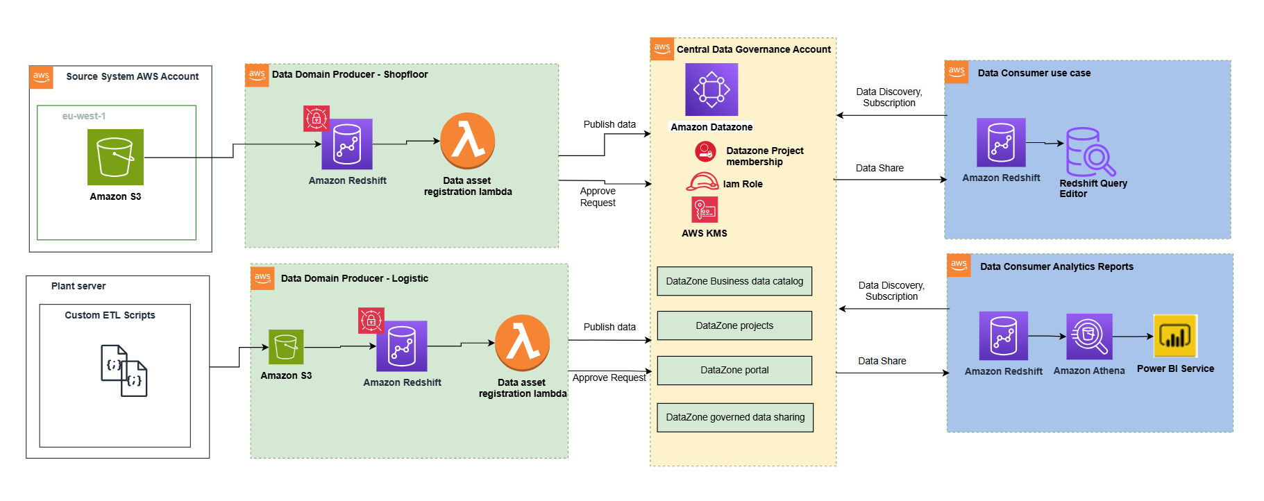
This architecture allows for the integration of multiple data warehouses into a centralized governance account that stores all the metadata from each environment.
A data domain producer uses Amazon Redshift as their analytical data warehouse to store, process, and manage structured and semi-structured data. The data domain producers load data into their respective Amazon Redshift clusters through extract, transform, and load (ETL) pipelines they manage, own, and operate. The producers maintain control over their data through Amazon Redshift security features, including column-level access controls and dynamic data masking, supporting data governance at the source. A data domain producer uses Amazon Redshift ETL and Amazon Redshift Spectrum to process and transform raw data into consumable data products. The data products could be Amazon Redshift tables, views, or materialized views.
Data domain producers expose datasets to the rest of the organization by registering them to Amazon DataZone service, which acts as a central data catalog. They can choose what data assets to share, for how long, and how consumers can interact with these. They’re also responsible for maintaining the data and making sure it’s accurate and current.
The data assets from the producers are then published using the data source run to Amazon DataZone in the central governance account. This process populates the technical metadata into the business data catalog for each data asset. The business metadata can be added by business users (data analysts) to provide business context, tags, and data classification for the datasets. This approach provides the required features to allow producers to create catalog entries with Amazon Redshift from all their data warehouses built in with Redshift clusters. In addition, the central data governance account is used to share datasets securely between producers and consumers. It’s important to note that sharing is done through metadata linking alone. No data (except logs) exists in the governance account. The data isn’t copied to the central account; just a reference to the data is used, so that the data ownership remains with the producer.
Amazon DataZone provides a streamlined way to search for data. The Amazon DataZone data portal provides a personalized view for users to discover and search data assets. An Amazon DataZone user (consumer) with permissions to access the data portal can search for assets and submit requests for subscription of data assets using a web-based application. An approver can then approve or reject the subscription request.
When a data domain consumer has access to an asset in the catalog, they can consume it (query and analyze) using the Amazon Redshift query editor. Each consumer runs their own workload based on their use case. In this way, the team can choose the tools for the job to perform analytics and machine learning activities in its AWS consumer environment.
Publishing and registering data assets to Amazon DataZone
To publish a data asset from the producer account, each asset must be registered in Amazon DataZone for consumer subscription. For more information, refer to Create and run an Amazon DataZone data source for Amazon Redshift. In the absence of an automated registration process, required tasks must be completed manually for each data asset.
Using the automated registration workflow, the manual steps can be automated for the Amazon Redshift data asset (Redshift table or view) that needs to be published in an Amazon DataZone domain or when there’s a schema change in an already published data asset.
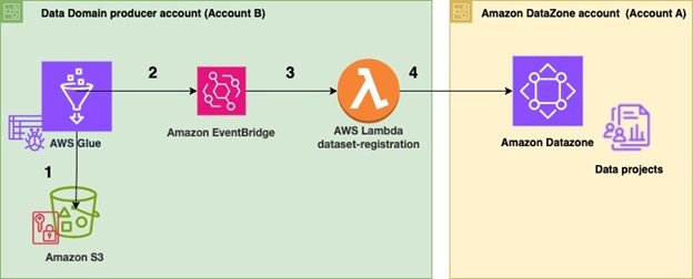
The following architecture diagram represents how data assets from Amazon Redshift data warehouses have been automatically published to the data mesh created with Amazon DataZone.
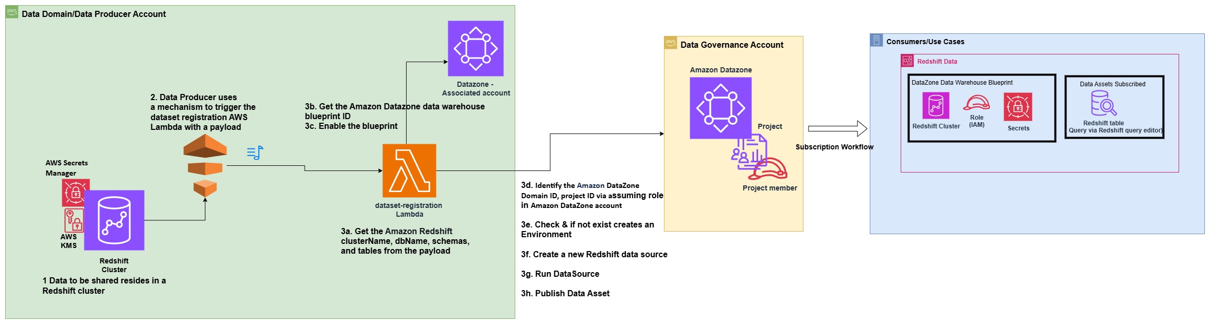
The process consists of the following steps:
- In the producer account (Account B), the data to be shared resides in a Redshift cluster.
- The producer account (Account B) uses a mechanism to trigger the dataset registration AWS Lambda function with a specific payload containing the information and name of the database, schema, table, or view that has a change in metadata.
- The Lambda function performs the steps to automatically register and publish the dataset in Amazon DataZone:
- Get the Amazon Redshift clusterName, dbName, schemas, and tables from the JSON payload, which is used as the event to trigger the Lambda function.
- Get the Amazon DataZone data warehouse blueprint ID.
- Enable the blueprint in the data producer account.
- Identify the Amazon DataZone Domain ID and project ID for the producer via assuming role in Amazon DataZone account (Account A).
- Check if an environment already exists in the project. If not, create an environment.
- Create a new Redshift data source by providing the correct Redshift database information in the newly created environment.
- Initiate a data source run request in the data source to make the Redshift tables or views available in Amazon DataZone.
- Publish the tables or views in the Amazon DataZone catalog.
Prerequisites
The following prerequisites are required before starting:
- Two AWS accounts to implement the solution have been described in this post. However, you can also use Amazon DataZone to publish data within a single account or across multiple accounts.
- Amazon DataZone account (Account A) – This is the central data governance account, which will have the Amazon DataZone domain and project.
- Data domain producer account (Account B) – This account acts as the data domain producer. It has been added as an associated account to Account A.
Prerequisites in data domain producer account (Account B)
As part of this post, we want to publish assets and subscribe to assets from a Redshift cluster that already exists. Complete the following prerequisite steps to set up Account B:
- Set up the Redshift cluster, including database, schema, tables, and views (optional). The node type must be from the RA3 family. For more information, see Amazon Redshift provisioned clusters.
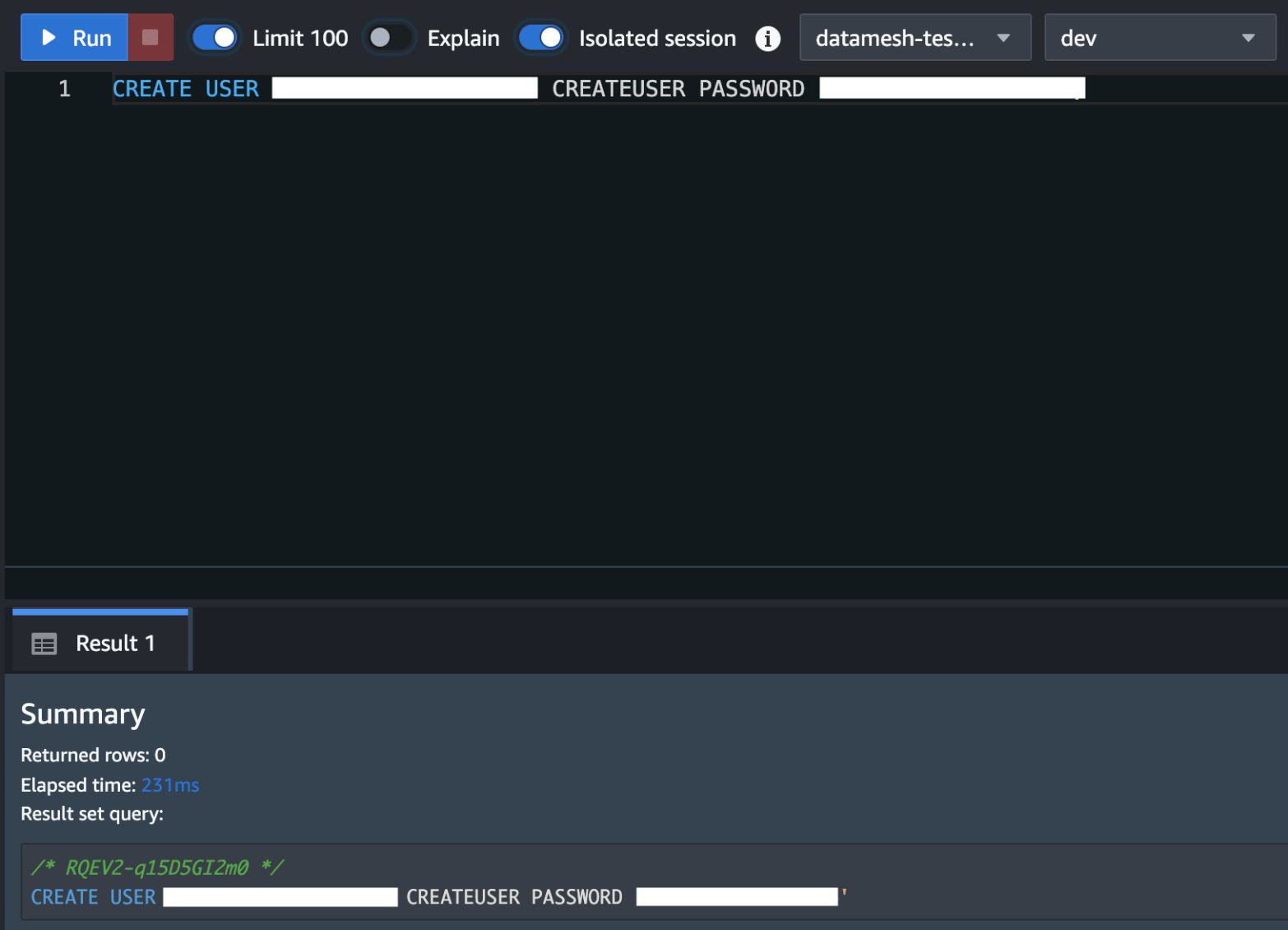
Create a superuser in Amazon Redshift for Amazon DataZone. For the Redshift cluster, the database user you provide in AWS Secrets Manager must have superuser permissions. For reference please see the note section in this QuickStart guide with sample Amazon Redshift data

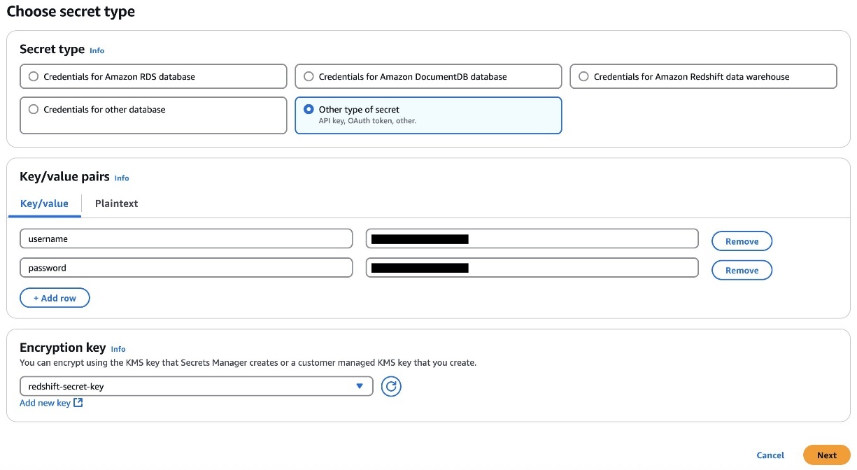
- Store the user’s credentials in Secrets Manager. Select the credential type, enter the credential values, and choose the AWS Key Management Service (AWS KMS) key with which to encrypt the secret.
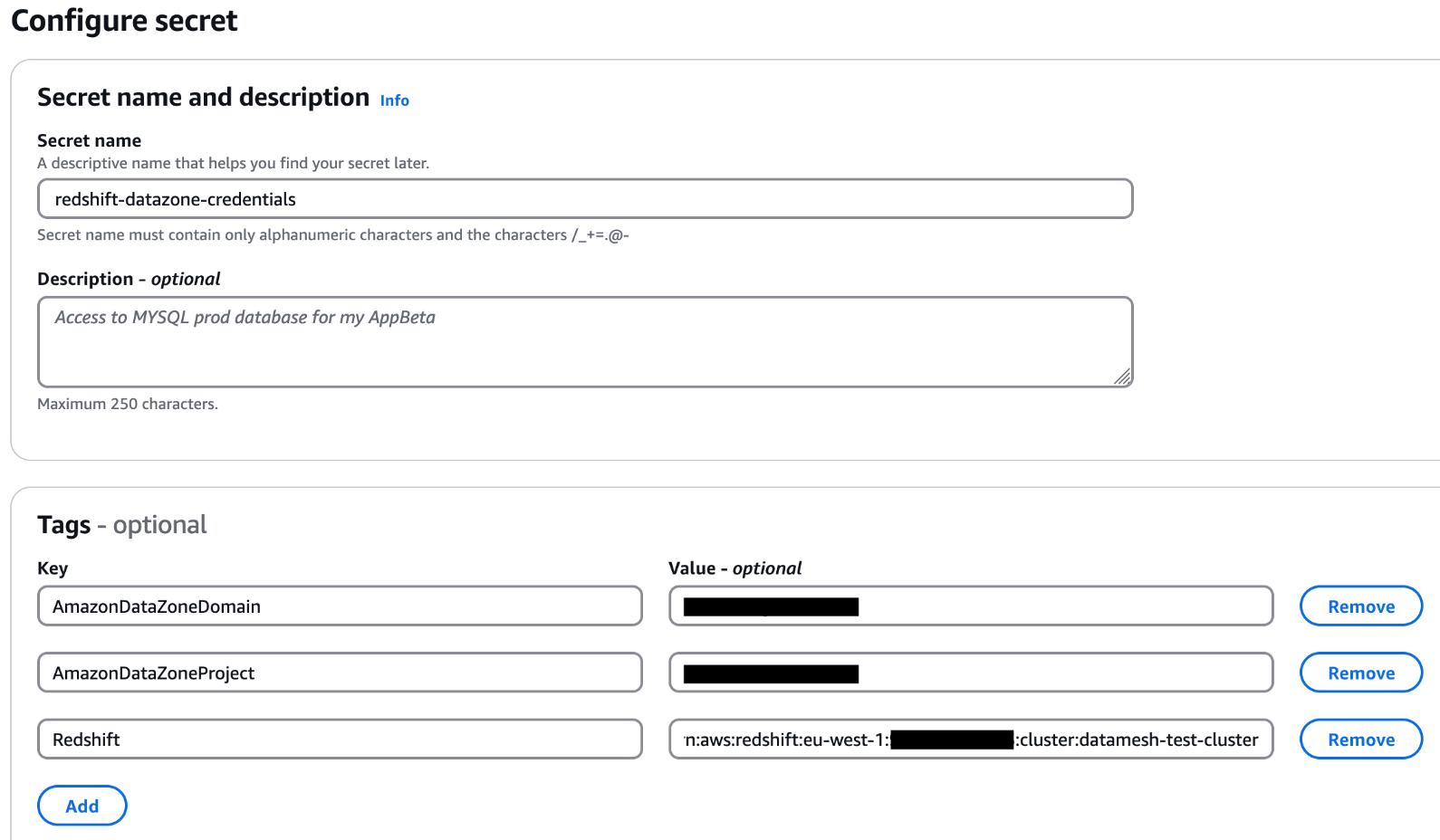
- Add the tags to the Secret Manager secret to allow Amazon DataZone to find this secret and limit the access to a particular Amazon DataZone domain and Amazon DataZone project. The Redshift cluster Amazon Resource Name (ARN) must be added as a tag so it can be used by Amazon Redshift as a valid credential. For reference please see the note section in this QuickStart guide with sample Amazon Redshift data
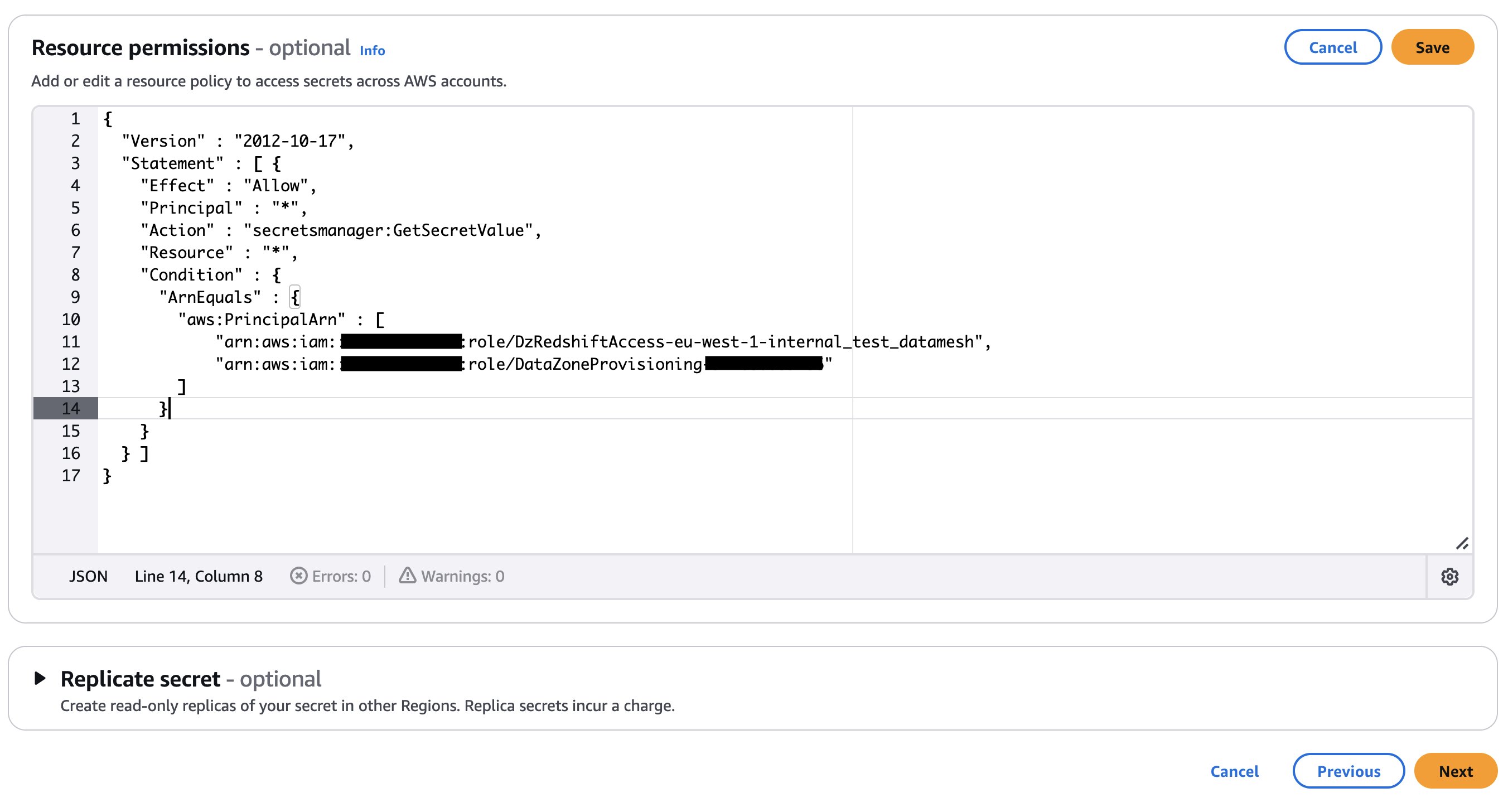
- Add an Amazon DataZone provisioning IAM role and Amazon Redshift manage access IAM role in the secret’s resource policy. The AWS Identity and Access Management (IAM) roles are created as part of the AWS Cloud Development Kit (AWS CDK) deployment (discussed later in this post). The following code shows an example of the Secrets Manager secret’s resource policy. Store the secret ARN in an AWS Systems Manager parameter.
If your secret is encrypted with a custom KMS key, append the key policy with the following statement and add a tag to the key:
AmazonDatazoneEnvironment = All. You can skip this step if you’re using an AWS managed KMS key. - Place a mechanism to generate the following payload to trigger the dataset registration Lambda function. The payload must contain the relevant Redshift database, schema, and table or view that you want to publish in the Amazon DataZone domain. The following example code assumes you have three databases in your Redshift cluster and within those databases you have different schemas, tables, and views. You should adjust the payload based on your use case.
 If your secret is encrypted with a custom KMS key, append the key policy with the following statement and add a tag to the key:
 Prerequisites in Amazon DataZone account (Account A)
Complete the following steps to set up your Amazon DataZone account (Account A):
- Sign in to Account A and make sure you have already deployed an Amazon DataZone domain and a project within that domain. Refer to Create Amazon DataZone domains for instructions to create a domain.
- If your Amazon DataZone domain is encrypted with a KMS key, add the data domain account (Account B) to the KMS key policy with the following actions:
- Create an IAM role that is assumable by Account B and make sure the role has a following policy attached and is a member (as contributor) of your Amazon DataZone project. For this post, we call the role
dz-assumable-env-dataset-registration-role. By adding this role, you can successfully run the registration Lambda function.- In the following policy, provide the AWS Region and account ID corresponding to where your Amazon DataZone domain is created, and the KMS key ARN used to encrypt the domain:
- Add Account B in the trust relationship of this role with the following trust relationship:
- Add the role as a member of the Amazon DataZone project in which you want to register your data sources. For more information, see Add members to a project.
Additional tools
The following tools are needed to deploy the solution using the AWS CDK:
- Either Bash/ or ZSH terminal
- Node and NPM using Node Version Manager:
- Install Node Version Manager (NVM)
- Install Node version 18.12.0 using the following command (node and npm binaries should now be available):
- Python
- AWS Command Line Interface (AWS CLI); see Installing or updating to the latest version of the AWS CLI
- AWS CDK for Python (Boto3); see Installation
- AWS CDK
Deploy the solution
After you complete the prerequisites, use the AWS CDK stack provided on the GitHub repo to deploy the solution for automatic registration of data assets into the Amazon DataZone domain. Complete the following steps:
- Clone the repository from GitHub to your preferred integrated development environment (IDE) using the following commands:
- At the base of the repository folder, run the following commands to build and deploy resources to AWS:
- Sign in to Account B (the data domain producer account) using the AWS CLI with your profile name.
- Make sure you have configured the Region in your credential’s configuration file.
- Bootstrap the AWS CDK environment with the following commands at the base of the repository folder. Provide the profile name of your deployment account (Account B). Bootstrapping is a one-time activity and is not needed if your AWS account is already bootstrapped.
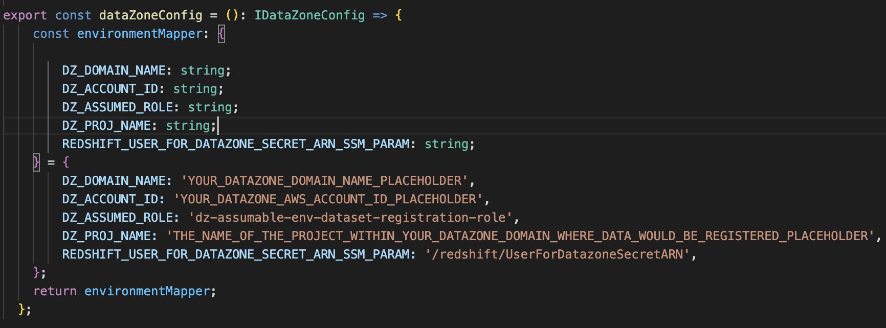
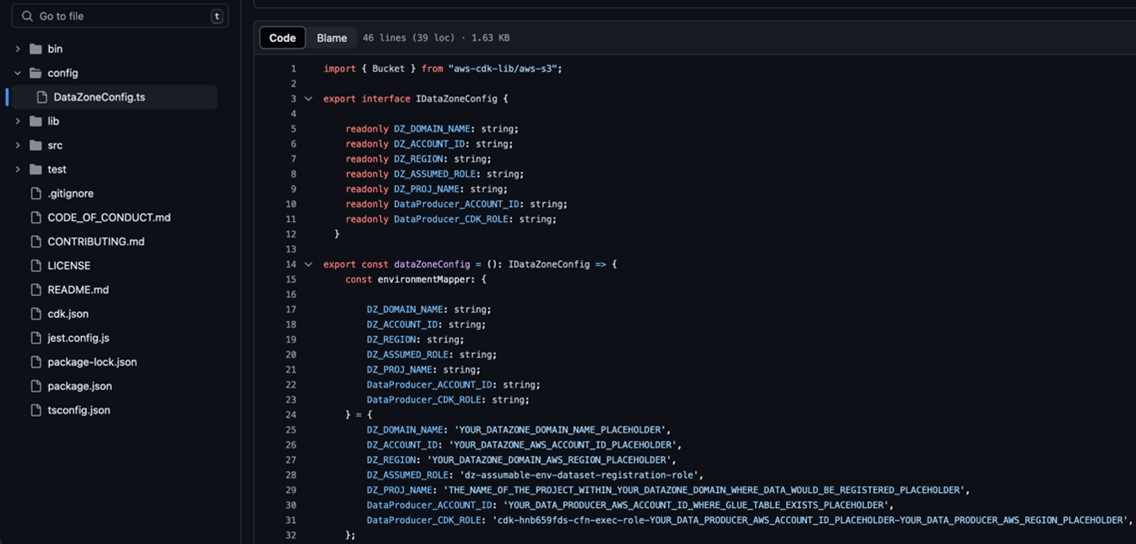
- Replace the placeholder parameters (marked with the suffix
_PLACEHOLDER) in the fileconfig/DataZoneConfig.ts:- Amazon DataZone domain and project name of your Amazon DataZone instance. Make sure all names are in lowercase.
- The AWS account ID of the Amazon DataZone account (Account A).
- The assumable IAM role from the prerequisites.
- The AWS Systems Manager parameter name containing the Secrets Manager secret ARN of the Amazon Redshift credentials.
- Use the following command in the base folder to deploy the AWS CDK solution. During deployment, enter
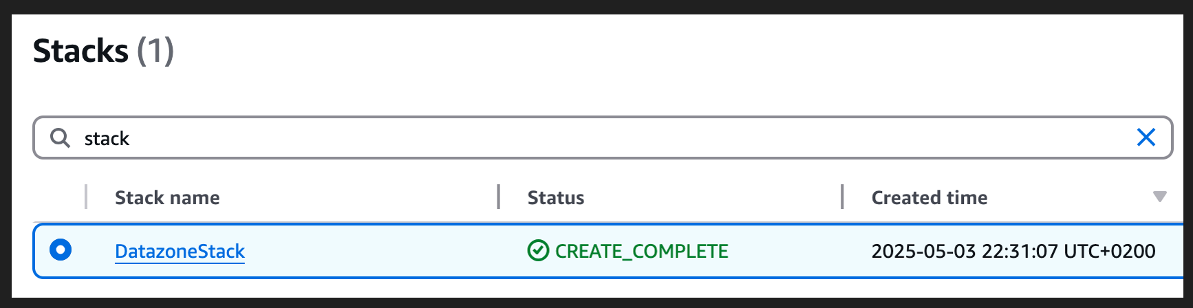
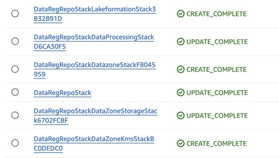
yif you want to deploy the changes for some stacks when you see the promptDo you wish to deploy these changes (y/n)? - After the deployment is complete, sign in to Account B and open the AWS CloudFormation console to verify that the infrastructure was deployed.
Test automatic data registration to Amazon DataZone
Complete the following steps to test the solution:
- Sign in to Account B (producer account).
- On the Lambda console, open the
datazone-redshift-dataset-registrationfunction. - Under TEST EVENTS, choose Create new test event.
- For Event name, enter
Redshift, and for Event JSON, enter the following JSON structure (change the cluster, schema, database, and table names according to your environment): - Choose Save.
- Choose Invoke.
- Open the Amazon DataZone console in Account A where you deployed the resources.
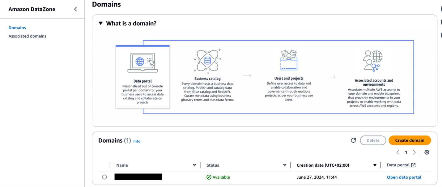
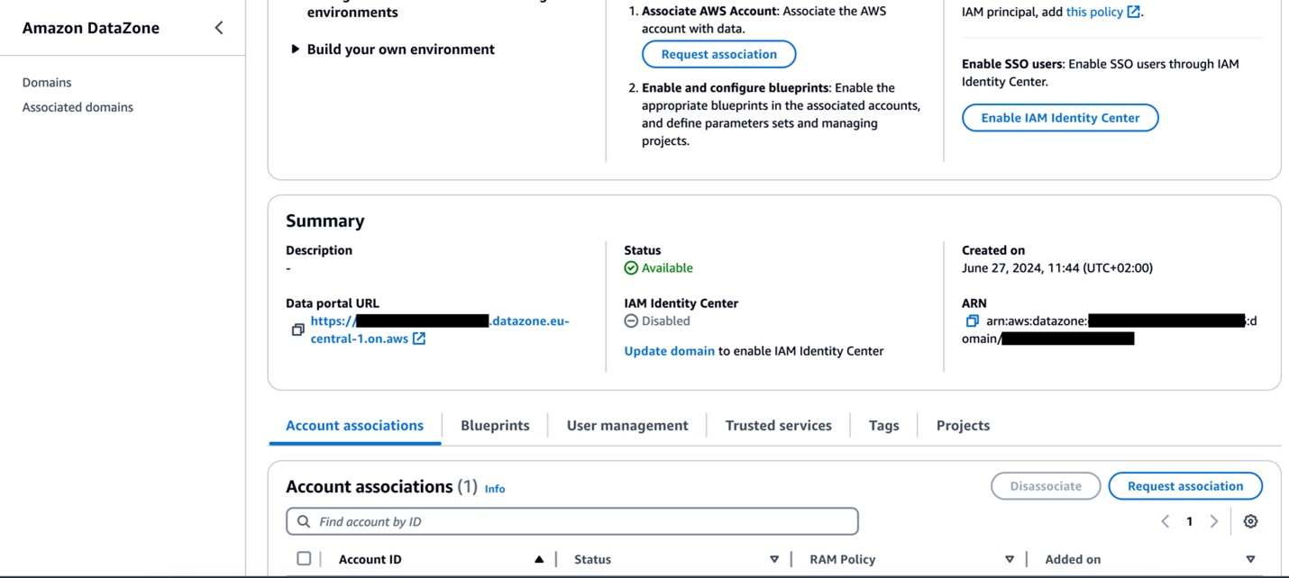
- Choose Domains in the navigation pane, then open your domain.
- On the domain details page, locate the Amazon DataZone data portal URL in the Summary section. Choose the link to the data portal.
For more details about accessing Amazon DataZone, refer to How can I access Amazon DataZone?
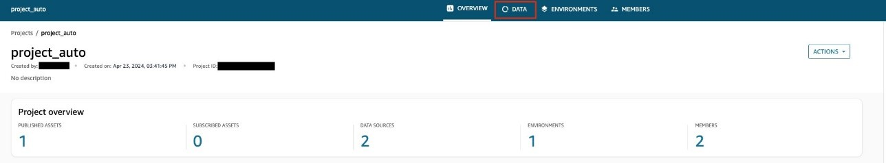
- In the data portal, open your project and choose the Data tab.
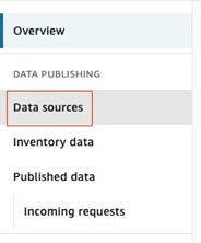
- In the navigation pane, choose Data sources and find the newly created data source for Amazon Redshift.
- Verify that the data source has been successfully published.

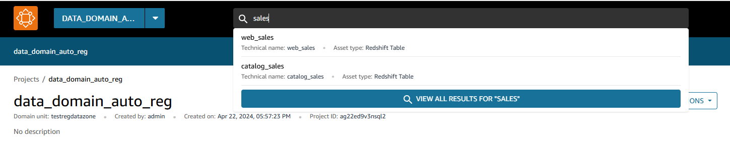
After the data sources are published, users can discover the published data and submit a subscription request. The data producer can approve or reject requests. Upon approval, users can consume the data by querying the data in the Amazon Redshift query editor. The following screenshot illustrates data discovery in the Amazon DataZone data portal.
Clean up
Complete the following steps to clean up the resources deployed through the AWS CDK:
- Sign in to Account B, go to the Amazon DataZone domain portal, and check there is no subscription for your published data asset. If there is a subscription, either ask the subscriber to unsubscribe or revoke the subscription request.
- Delete the published data assets that were created in the Amazon DataZone project by the dataset registration Lambda function.
- Delete the remaining resources created using the following command in the base folder:
Conclusion
Amazon DataZone offers a seamless integration with AWS services, providing a powerful solution for organizations like Volkswagen to break down their data silos and implement effective data mesh architectures through a straightforward implementation highlighted in this post. By using Amazon DataZone, Volkswagen addressed its immediate data sharing hurdles and laid the groundwork for a more agile, data-driven future in automotive manufacturing. The automated data publishing from various warehouses, coupled with standardized governance workflows, has significantly reduced the manual overhead that once slowed down Volkswagen’s data engineering teams. Now, instead of navigating a labyrinth of emails, tickets, and communication, Volkswagen’s data engineers and data scientists can quickly discover and access the data they need, all while maintaining their security and compliance standards.
By using Amazon DataZone, organizations can bring their isolated data together in ways that make it simpler for teams to collaborate while maintaining security and compliance at scale. This approach not only addresses current data governance challenges but also creates a highly scalable foundation for future data-driven innovations. For guidance on establishing your organization’s data mesh with Amazon DataZone, contact your AWS team today.


 Dhrubajyoti Mukherjee is a Cloud Infrastructure Architect with a strong focus on data strategy, data analytics, and data governance at Amazon Web Services (AWS). He uses his deep expertise to provide guidance to global enterprise customers across industries, helping them build scalable and secure AWS solutions that drive meaningful business outcomes. Dhrubajyoti is passionate about creating innovative, customer-centric solutions that enable digital transformation, business agility, and performance improvement. An active contributor to the AWS community, Dhrubajyoti authors AWS Prescriptive Guidance publications, blog posts, and open-source artifacts, sharing his insights and best practices with the broader community. Outside of work, Dhrubajyoti enjoys spending quality time with his family and exploring nature through his love of hiking mountains.
 Ravi Kumar is a Data Architect and Analytics expert at Amazon Web Services; he finds immense fulfillment in working with data. His days are dedicated to designing and analyzing complex data systems, uncovering valuable insights that drive business decisions. Outside of work, he unwinds by listening to music and watching movies, activities that allow him to recharge after a long day of data wrangling.
 Martin Mikoleizig studied mechanical engineering and production technology at the RWTH Aachen University before starting to work in Dr. h.c. Ing. F. Porsche AG 2015 as a production planner for the engine assembly. In several years as a Project Manager on Testing Technology for new engine models he also introduced several innovations like human-machine-collaborations and intelligent assistance systems. From 2017, he was responsible for the Shopfloor IT team of the module lines in Zuffenhausen before he became responsible for the Planning of the E-Drive assembly at Porsche. Beside this he was responsible for the Digitalisation Strategy of the Production Ressort at Porsche. Since October 2022, he has been assigned to Volkswagen Autoeuropa in Portugal in the role of a Digital Transformation Manager for the plant driving the Digital Transformation towards a Data Driven Factory.
 Weizhou Sun is a Lead Architect at Amazon Web Services, specializing in digital manufacturing solutions and IoT. With extensive experience in Europe, she has enhanced operational efficiencies, reducing latency and increasing throughput. Weizhou’s expertise includes Industrial Computer Vision, predictive maintenance, and predictive quality, consistently delivering top performance and client satisfaction. A recognized thought leader in IoT and remote driving, she has contributed to business growth through innovations and open-source work. Committed to knowledge sharing, Weizhou mentors colleagues and contributes to practice development. Known for her problem-solving skills and customer focus, she delivers solutions that exceed expectations. In her free time, Weizhou explores new technologies and fosters a collaborative culture.
 Shameka Almond is an Advisory Consultant at Amazon Web Services. She works closely with enterprise customers to help them better understand the business impact and value of implementing data solutions, including data governance best practices. Shameka has over a decade of wide-ranging IT experience in the manufacturing and aerospace industries, and the nonprofit sector. She has supported several data governance initiatives, helping both public and private organizations identify opportunities for improvement and increased efficiency. Outside of the office she enjoys hosting large family gatherings, and supporting community outreach events dedicated to introducing students in K-12 to STEM.
 Adjoa Taylor has over 20 years of experience in industrial manufacturing, providing industry and technology consulting services, digital transformation, and solution delivery. Currently Adjoa leads Product Centric Digital Transformation, enabling customers to solve complex manufacturing problems by leveraging Smart Factory and Industry leading transformation mechanisms. Most recently driving value with AI/ML and generative AI use-cases for the plant floor. Adjoa is an experienced leader spending over 20 years of her career delivering projects in countries throughout North America, Latin America, Europe, and Asia. Through prior roles, Adjoa brings deep experience across multiple business segments with a focus on business outcome driven solutions. Adjoa is passionate about helping customers solve problems while realizing the art of the possible via the right impacting value-based solution.
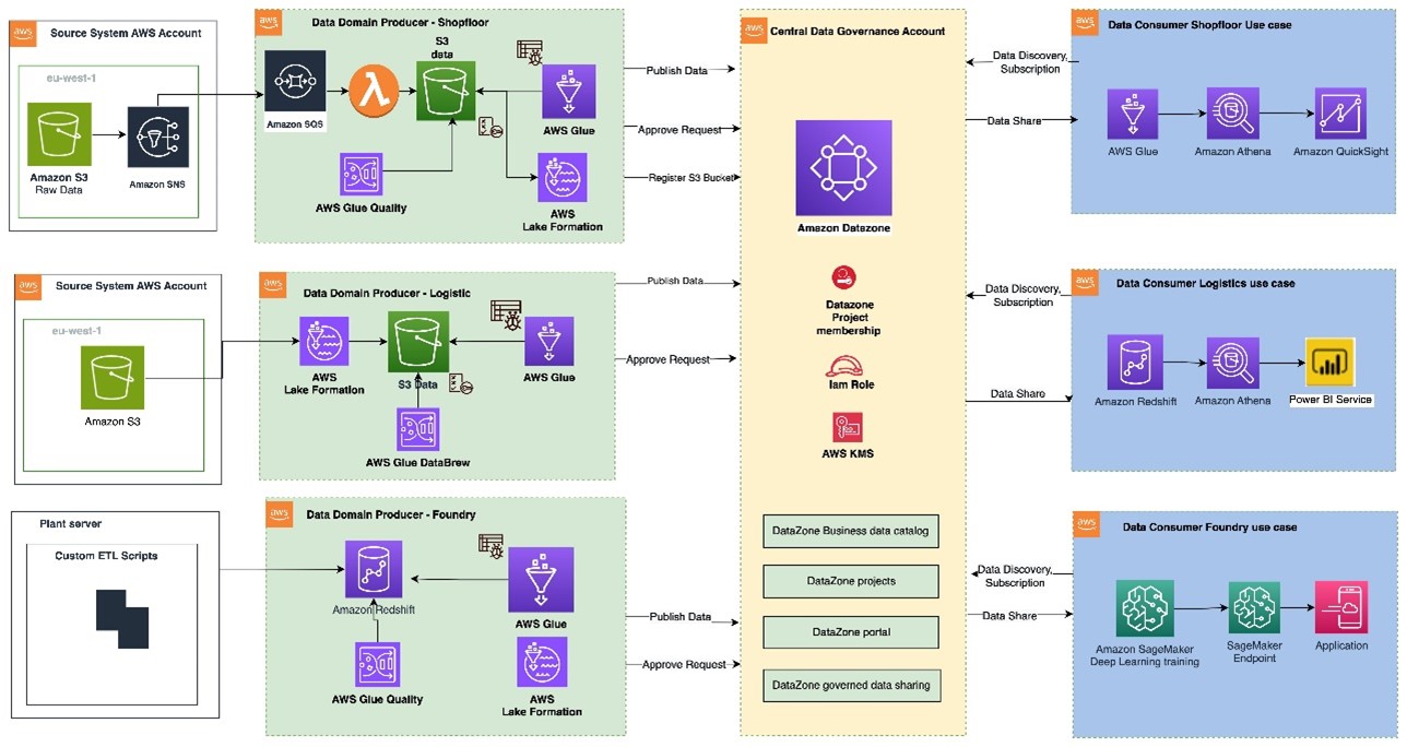


 Bandana Das is a Senior Data Architect at Amazon Web Services and specializes in data and analytics. She builds event-driven data architectures to support customers in data management and data-driven decision-making. She is also passionate about enabling customers on their data management journey to the cloud.
 Anirban Saha is a DevOps Architect at AWS, specializing in architecting and implementation of solutions for customer challenges in the automotive domain. He is passionate about well-architected infrastructures, automation, data-driven solutions and helping make the customer’s cloud journey as seamless as possible. Personally, he likes to keep himself engaged with reading, painting, language learning and traveling.
 Chandana Keswarkar is a Senior Solutions Architect at AWS, who specializes in guiding automotive customers through their digital transformation journeys by using cloud technology. She helps organizations develop and refine their platform and product architectures and make well-informed design decisions. In her free time, she enjoys traveling, reading, and practicing yoga.
 Sindi Cali is a ProServe Associate Consultant with AWS Professional Services. She supports customers in building data driven applications in AWS.


 Figure 1. AVA displays anomalies raised from L4E. A prediction score of > 0 indicates that an anomaly has been detected, and AVA will raise an issue with the underlying sensor details.