All posts by Steve Phillips

AI-powered performance recommendations for Amazon Redshift

Post Syndicated from Steve Phillips original https://aws.amazon.com/blogs/big-data/ai-powered-performance-recommendations-for-amazon-redshift/

Data platform teams running Amazon Redshift collect performance telemetry across system views like SYS_QUERY_HISTORY, SVV_TABLE_INFO, and SVV_ALTER_TABLE_RECOMMENDATIONS, plus Amazon CloudWatch metrics for capacity, query execution, and storage. The challenge is interpretation. Correlating a spike in QueryRuntimeBreakdown commit time with hundreds of small INSERT statements, or connecting high disk spill with undersized compute, takes deep expertise and hours of manual analysis.

In this post, you learn how to build an AI-powered solution that collects the telemetry, pre-computes performance signals, correlates them with CloudWatch, and uses Amazon Bedrock to generate prioritized recommendations. The source code is in the accompanying GitHub repository: sample-ai-performance-advisor-for-amazon-redshift.

The signal-based design is what makes this solution produce precise recommendations rather than generic advice. Instead of dumping raw system view output into the large language model (LLM) prompt, the collector pre-computes boolean and threshold-based findings, pairs them with CloudWatch correlations, and hands the model a structured context. The model then cross-references specific query IDs, table names, and metric values in its output.

Solution overview

Two AWS Lambda functions run on a 24-hour Amazon EventBridge schedule:

  • The collector Lambda runs 13 diagnostic SQL queries against Amazon Redshift Serverless and reads the workgroup’s Workload Management (WLM) configuration. It also collects CloudWatch metrics across capacity, query execution, WLM, connections, and storage. From these inputs, it computes the performance signals. Finally, it writes a telemetry JSON file to Amazon Simple Storage Service (Amazon S3).
  • The analyzer Lambda reads the telemetry from Amazon S3, builds a structured prompt with inline CloudWatch-to-signal correlations. Using the correlations, the analyzer calls Amazon Bedrock (Anthropic Claude Sonnet 4.6), and writes the resulting recommendations JSON back to Amazon S3.
  • An Amazon Simple Notification Service (Amazon SNS) topic sends an email summary of the top recommendations to subscribers.
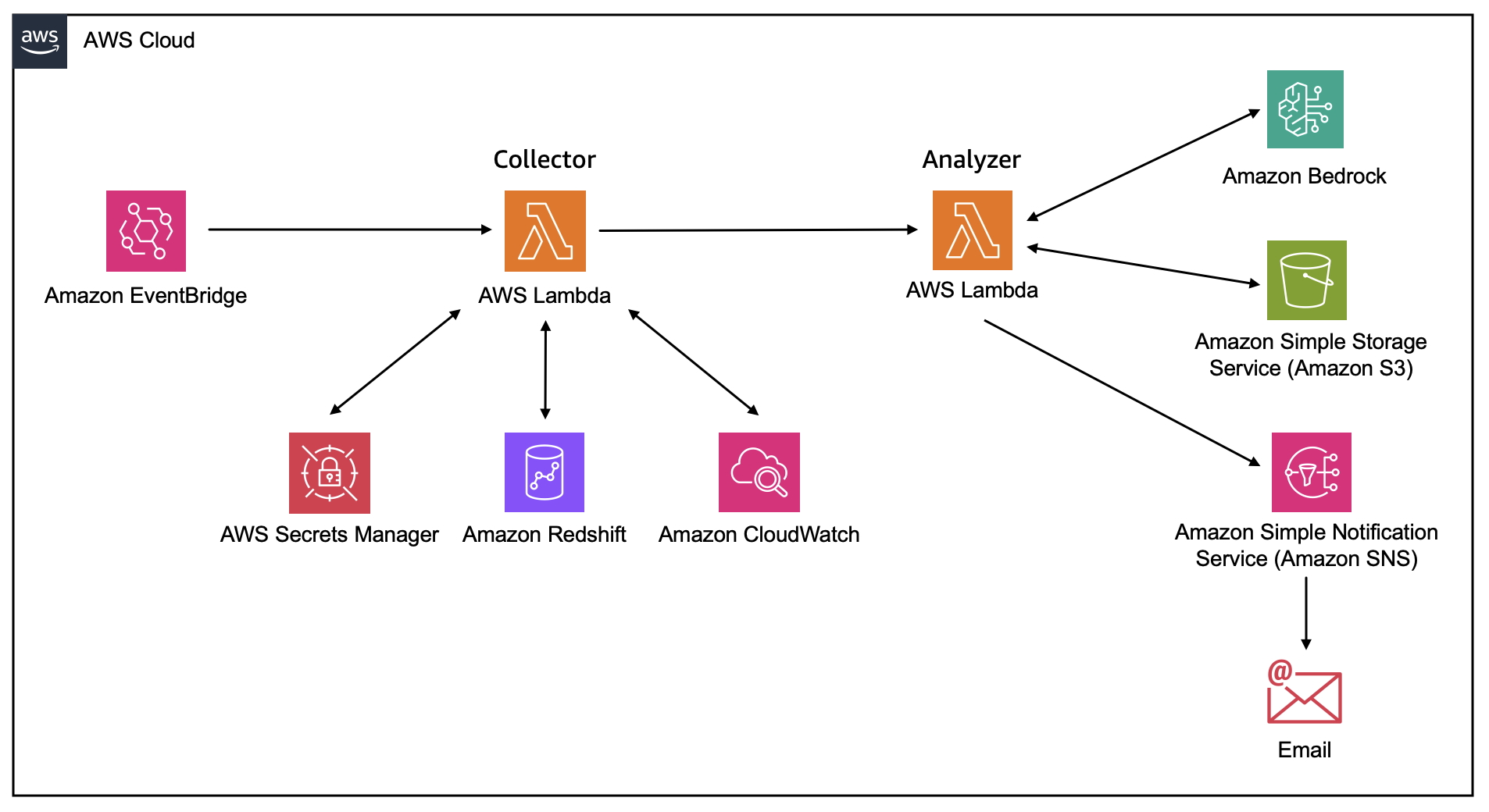
AWS architecture diagram showing an automated Redshift analysis pipeline within the AWS Cloud. Amazon EventBridge triggers a “Collector” AWS Lambda function, which interacts bidirectionally with AWS Secrets Manager, Amazon Redshift, and Amazon CloudWatch to gather data. The Collector passes results to an “Analyzer” AWS Lambda function, which exchanges data with Amazon Bedrock and reads/writes to Amazon S3. The Analyzer then publishes to Amazon Simple Notification Service (SNS), which delivers an email notification.

Figure 1 – Architecture diagram

Prerequisites

Before deploying the solution, make sure the following are in place.

  • An Amazon Redshift Serverless workgroup with a database and query history.
  • An Amazon Redshift database administrator user (superuser). The collector reads views that only a superuser can query (SVV_TABLE_INFO, SVV_ALTER_TABLE_RECOMMENDATIONS, SVV_MV_INFO, SYS_SERVERLESS_USAGE, SYS_AUTO_TABLE_OPTIMIZATION).
    Store the admin credentials in AWS Secrets Manager and pass the secret ARN to the collector.
    Alternatively, have an existing superuser run ALTER USER "IAMR:redshift-performance-recommendations-role" CREATEUSER;
    once to grant the Lambda role superuser privileges.
  • Amazon Bedrock model access for the model of choice. For this solution, a us.anthropic.claude-* model is recommended for multi-region inference. The solution doesn’t depend on a single model.
  • The AWS Command Line Interface (AWS CLI) installed and configured, and a clone of the GitHub repository.

Create the supporting resources

You need an Amazon S3 bucket, an Amazon SNS topic, an AWS Secrets Manager secret, and an AWS Identity and Access Management (IAM) role before the Lambda functions can run.

Create the Amazon S3 bucket

The Amazon S3 bucket will host the output report.

  • Open the Amazon S3 console and choose Create bucket.
  • Enter a globally unique name (for example, amzn-s3-demo-bucket), keep the default settings, and choose Create bucket.

The collector writes telemetry JSON under the telemetry/ prefix and the analyzer writes recommendations under the recommendations/ prefix.

Create the Amazon SNS topic and subscription

Use Amazon SNS to generate notifications once reports are created.

  • Open the Amazon SNS console and choose Topics, Create topic.
  • Select Standard, and enter the name redshift-performance-recommendations.
  • Choose Create topic.
  • On the topic detail page, choose Create subscription.
  • Select Email as the protocol, enter your email address, and choose Create subscription.
  • Open the confirmation email from AWS Notifications and choose Confirm subscription.
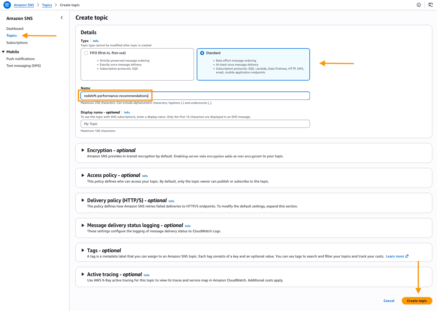
Amazon SNS “Create topic” console page. The Type is set to Standard (selected over FIFO), and the Name field contains “redshift-performance-recommendations.” Annotation arrows highlight the Topics nav item, the Standard topic type, the entered name, and the “Create topic” button in the lower right. Optional sections for Encryption, Access policy, Delivery policy, Message delivery status logging, Tags, and Active tracing are collapsed below.

Figure 2 – Create SNS Topic

Store the admin credentials in AWS Secrets Manager

To avoid using hard-coded credentials, create an AWS Secrets Manager secret to connect to Amazon Redshift.

  • Open the AWS Secrets Manager console and choose Store a new secret.
  • Select Other type of secret, choose the Plaintext tab, and paste the following, replacing <ADMIN_PASSWORD> with the workgroup’s admin password:
    {"username":"admin","password":"<ADMIN_PASSWORD>"}

  • Choose Next, enter redshift-performance-admin as the secret name, then choose Next, Next, and Store.
  • Copy the secret Amazon Resource Name (ARN) from the secret detail page. You pass it to the collector in a later step.
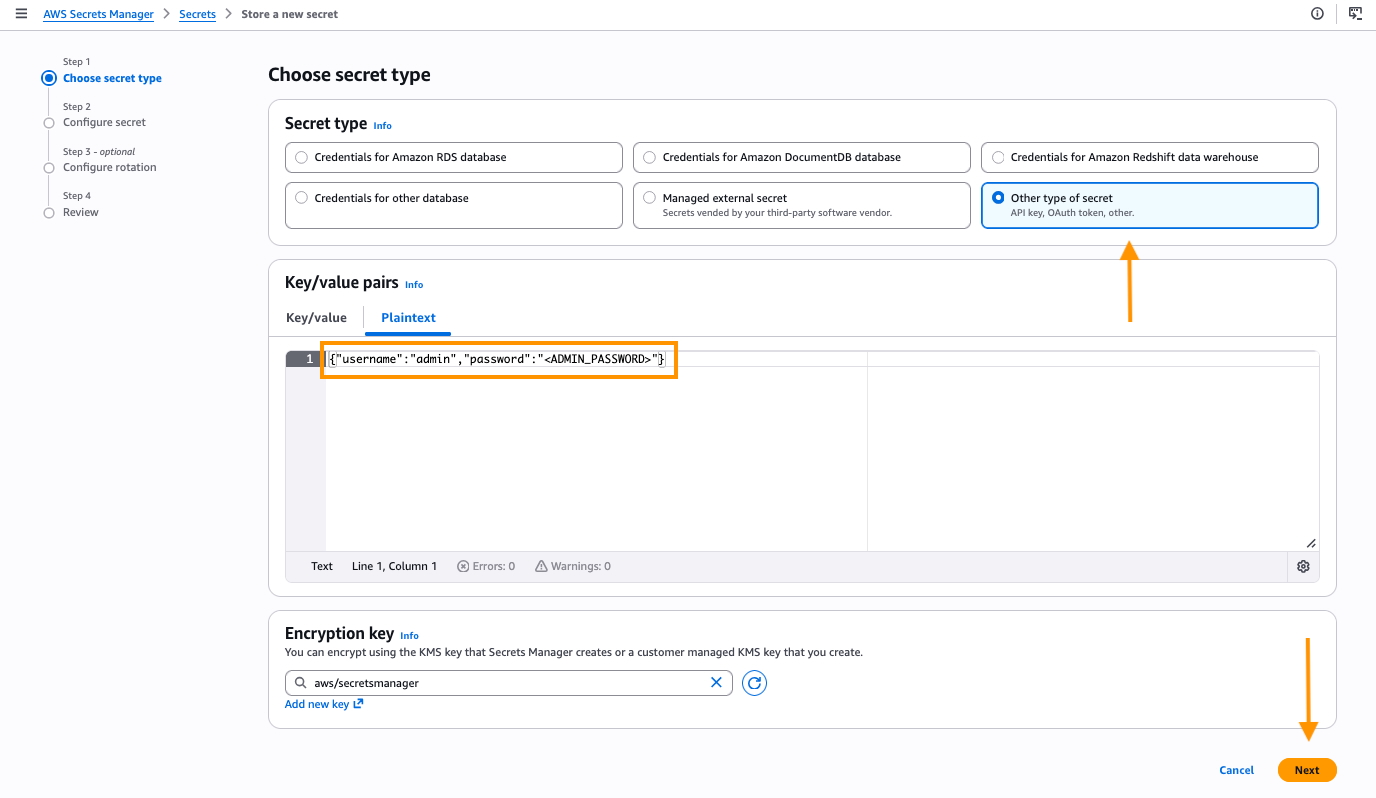
AWS Secrets Manager “Store a new secret” page, Step 1: Choose secret type. “Other type of secret” is selected, and the Plaintext tab shows the key-value pair {“username”:“admin”,“password”:“”}. The encryption key is set to aws/secretsmanager. Annotation arrows highlight the secret type selection, the plaintext credentials, and the “Next” button in the lower right.

Figure 3 – Create secret

Create the IAM role and attach the policy

The repository includes a trust policy in iam/trust-policy.json (allowing lambda.amazonaws.com to assume the role) and the least-privilege permission policy in iam/lambda-role-policy.json. Replace the <ACCOUNT_ID>, <REGION>, <YOUR_BUCKET>, and SNS topic ARN placeholders in the permission policy with your values, then create the role in the AWS Management Console or with this AWS CLI command:

aws iam create-role --role-name redshift-performance-recommendations-role \
    --assume-role-policy-document file://iam/trust-policy.json

aws iam put-role-policy --role-name redshift-performance-recommendations-role \
    --policy-name redshift-performance-policy \
    --policy-document file://iam/lambda-role-policy.json

The permission policy grants the Amazon Redshift Data API, Amazon S3, Amazon SNS, Amazon Bedrock, AWS Lambda invoke, AWS Secrets Manager, and Amazon CloudWatch Logs permissions that both Lambda functions require.

Deploy the Lambda functions

The collector source is in lambda/collector.py and it loads the SQL files in sql/ at runtime. The deployment package must contain both.

Package the collector

Open a terminal or shell window and execute a command to copy the collector code, supporting SQL into a folder and archive.

mkdir -p build/collector/sql
cp lambda/collector.py build/collector/
cp sql/*.sql build/collector/sql/
(cd build/collector && zip -qr ../collector.zip .)

Create the collector function

Using the AWS Management Console, navigate to AWS Lambda.

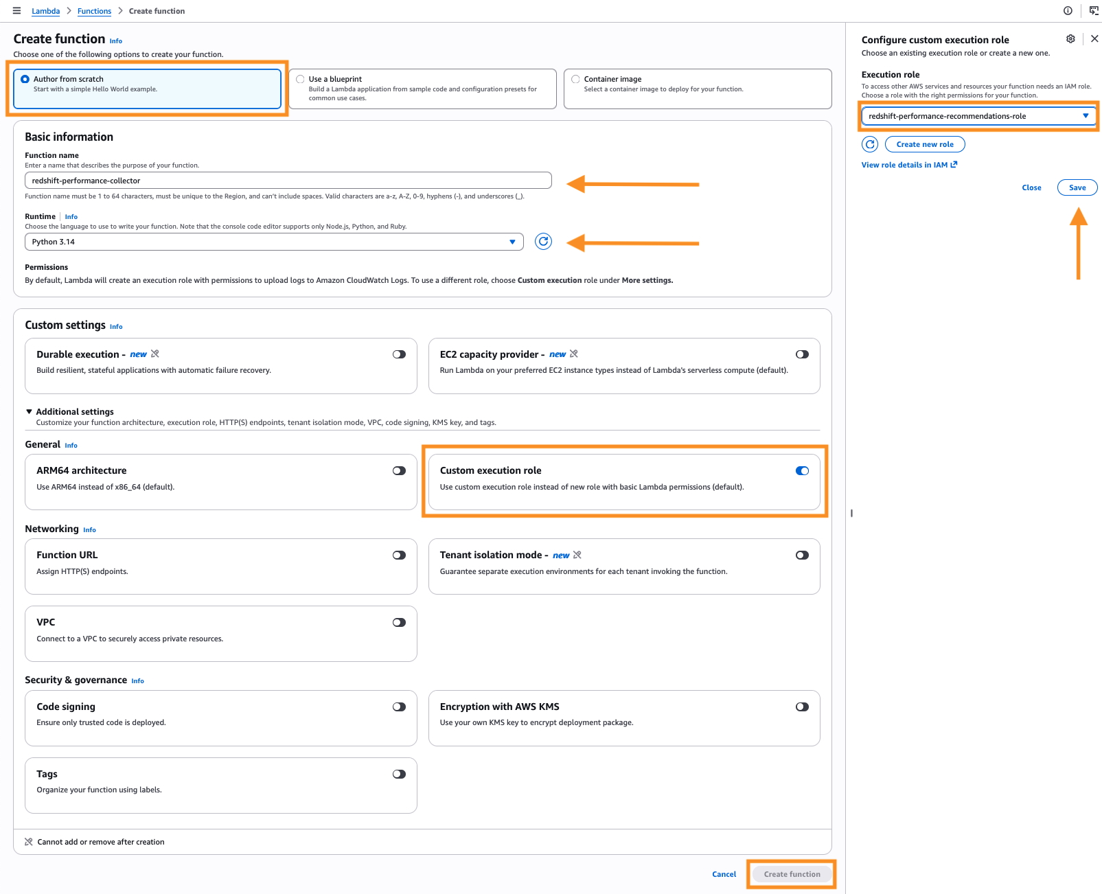
  • Choose Create function.

    AWS Lambda “Create function” console page with the “Configure custom execution role” panel open on the right. “Author from scratch” is selected, the function name is “redshift-performance-collector,” and the runtime is Python 3.14. Under Additional settings, the “Custom execution role” toggle is enabled, and the execution role list is set to “redshift-performance-recommendations-role.” Annotation highlights mark the Author from scratch option, function name, runtime, custom execution role toggle, the selected role, the Save button, and the “Create function” button.

    Figure 4 – Create AWS Lambda function

  • Select Author from scratch, enter redshift-performance-collector as the name, and select Python 3.14.
  • Expand Custom settings, toggle Custom execution role, choose an existing role, select redshift-performance-recommendations-role, and choose Save.
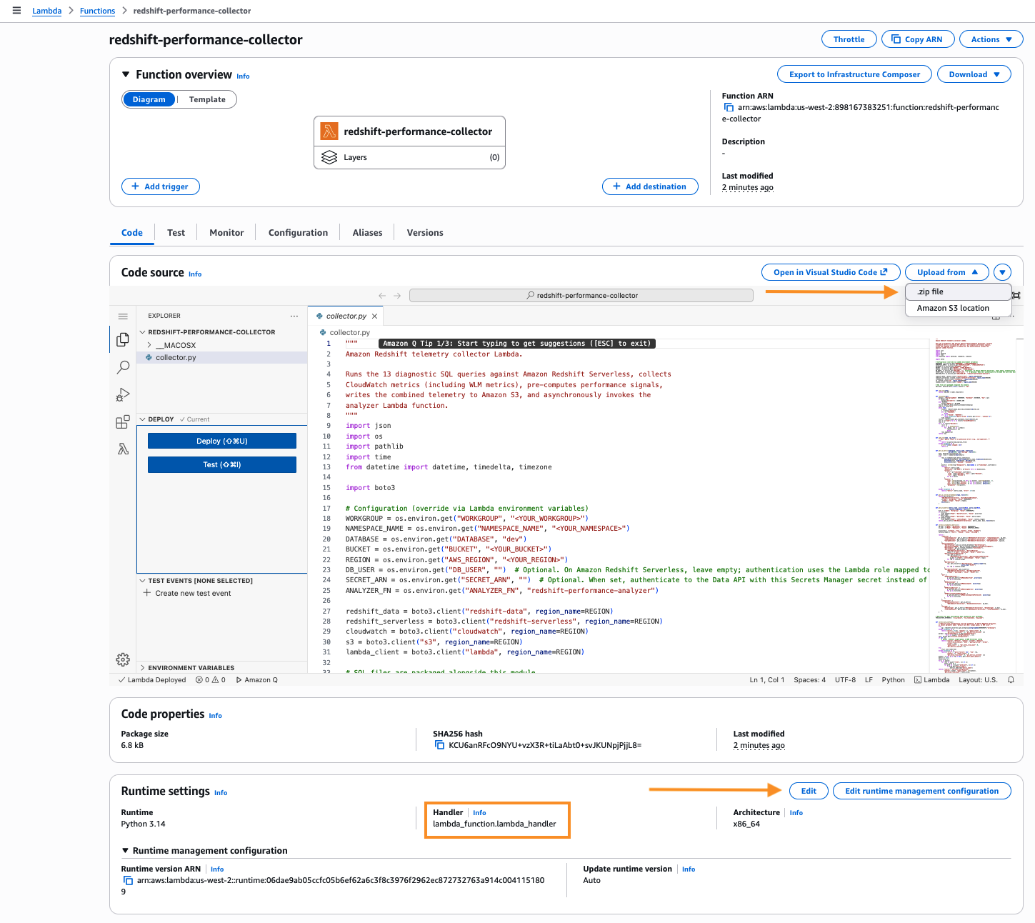
  • On the function page, choose Upload from, .zip file, and upload build/collector.zip.
  • In Runtime settings, select Edit, and set the Handler to collector.lambda_handler.

    Lambda console for the “redshift-performance-collector” function, Code tab. The code editor shows collector.py — a Python file that runs diagnostic SQL queries against Amazon Redshift Serverless, collects CloudWatch metrics, writes telemetry to Amazon S3, and invokes the analyzer Lambda. The Runtime settings section below shows the Handler highlighted as “lambda_function.lambda_handler,” with an arrow pointing to the Edit button and the “Upload from .zip file” option highlighted.

    Figure 5 – Set AWS Lambda handler

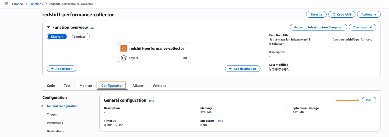
  • Choose Configuration, Edit, set timeout to 5 minutes, and memory to 256 MB.

    Lambda console for “redshift-performance-collector,” Configuration tab with “General configuration” selected. The panel shows Memory 128 MB, Ephemeral storage 512 MB, and Timeout 0 min 3 sec, with SnapStart set to None. Annotation arrows point to the General configuration menu item and the Edit button.

    Figure 6 – Set AWS Lambda timeout and memory

  • Under Configuration, select Environment variables, and add the following keys:
    • WORKGROUP: your Amazon Redshift Serverless workgroup name.
    • NAMESPACE_NAME: the namespace the workgroup belongs to.
    • DATABASE: dev (or your target database).
    • BUCKET: the Amazon S3 bucket name you created earlier.
    • SECRET_ARN: the AWS Secrets Manager secret ARN you copied earlier.
    • ANALYZER_FN: redshift-performance-analyzer.

Package and create the analyzer

Repeat the same steps for the analyzer, using lambda/analyzer.py with a 15-minute timeout:

(cd lambda && zip -q ../build/analyzer.zip analyzer.py)

Use the Lambda console to create redshift-performance-analyzer with handler analyzer.lambda_handler, timeout 15 minutes, memory 256 MB, the same execution role, and these environment variables:

  • BUCKET: the same Amazon S3 bucket.
  • SNS_TOPIC: the SNS topic ARN.
  • MODEL_ID: us.anthropic.claude-sonnet-4-6.

The analyzer creates the Amazon Bedrock client with read_timeout=600 and max_tokens=16384 to handle large prompts and long responses. Anthropic Claude inference on a full telemetry payload typically takes 2–4 minutes.

How the signals and the prompt work

You don’t write any custom code for signal computation or prompt construction. Both computation and construction live in the repository.

The compute_signals() function in lambda/collector.py scans the telemetry for Boolean and threshold-based anti-patterns. At the table level, it looks for row skew, ghost rows, stale statistics, unsorted data, sub-optimal sort or distribution keys, and oversized VARCHAR columns. It also flags runtime and workload issues such as disk spill, small-insert bursts, high Data Definition Language (DDL) executions, and unoptimized COPY file size. Beyond that, it catches Amazon Redshift Spectrum queries that fail to prune partitions and data sharing materialized views doing full refresh. It also flags WLM configurations that lack Query Monitoring Rules (QMR), such as limits on blocks spilled to disk and query execution time. The full set of signals and thresholds is defined inline in the function. To tune a threshold or add a custom signal, edit this function and redeploy.

The build_prompt() function in lambda/analyzer.py constructs the Amazon Bedrock prompt in four sections. The first section lists the triggered signals. The second adds CloudWatch metrics, annotated with >> CORRELATION lines that pair each signal with its supporting metric. The third includes the filtered supporting data, limited to the table and query rows that triggered a signal. The fourth gives explicit instructions to return a pipe delimited text where every recommendation references specific table names, query IDs, and metric values. This structure is why the model produces targeted output rather than generic best-practice advice.

Schedule daily runs

Use the Amazon EventBridge console to trigger the collector every 24 hours.

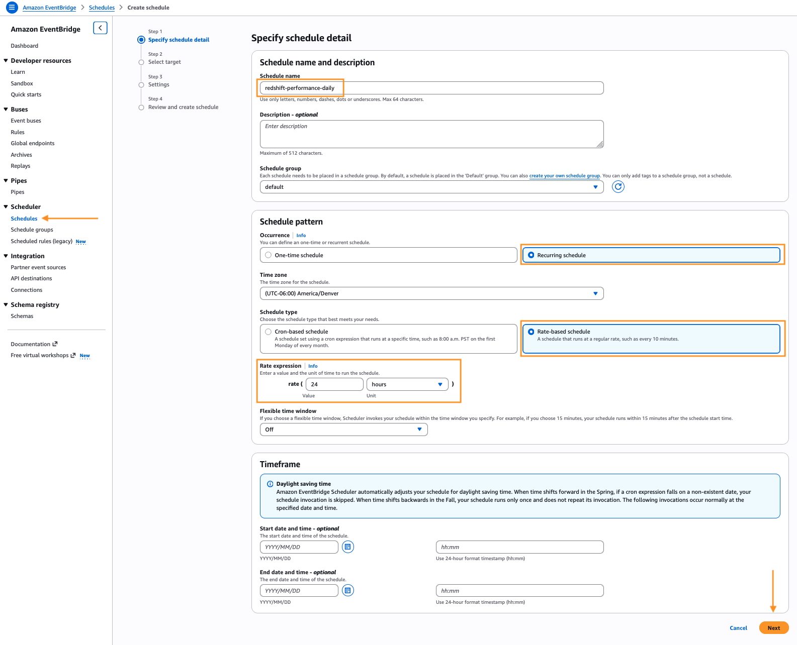
  • Open the EventBridge console and choose Schedules under Scheduler, Create schedule.
  • Enter the name redshift-performance-daily for Schedule name, toggle Recurring schedule and Rate-based schedule.
  • Under Rate expression, enter 24 and select hours.
  • For Flexible time window, choose Off, and select Next.
    Amazon EventBridge Scheduler “Create schedule” page, Step 1: Specify schedule detail. The schedule name is “redshift-performance-daily.” Under Schedule pattern, “Recurring schedule” and “Rate-based schedule” are selected, with a rate expression of 24 hours, and the time zone set to (UTC-06:00) America/Denver. Annotation highlights mark the Schedules nav item, the recurring/rate-based selections, the rate expression, and the Next button.

    Figure 7 – Create Amazon EventBridge schedule


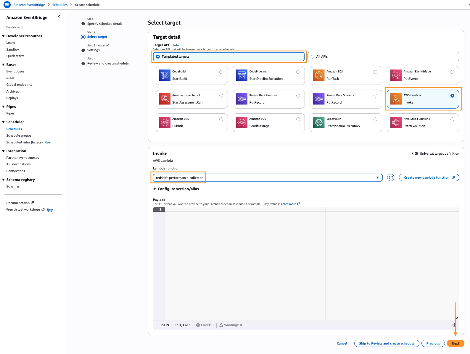
  • On the Select target page, choose AWS Lambda, select the redshift-performance-collector function, and choose Next.

    EventBridge Scheduler “Create schedule” page, Step 2: Select target. “Templated targets” is selected and the AWS Lambda “Invoke” target is chosen from the grid of target options. In the Invoke section, the Lambda function list is set to “redshift-performance-collector” with an empty JSON payload. Annotation highlights mark the Templated targets toggle, the AWS Lambda Invoke target, the selected function, and the Next button.

    Figure 8 – Select Amazon EventBridge schedule target

  • Accept the defaults for Settings and select Next. EventBridge automatically adds a resource-based permission on the Lambda function so the rule can invoke it.
  • Choose Create schedule.

Run it once and review the output

Invoke the collector manually to confirm the pipeline works end-to-end.

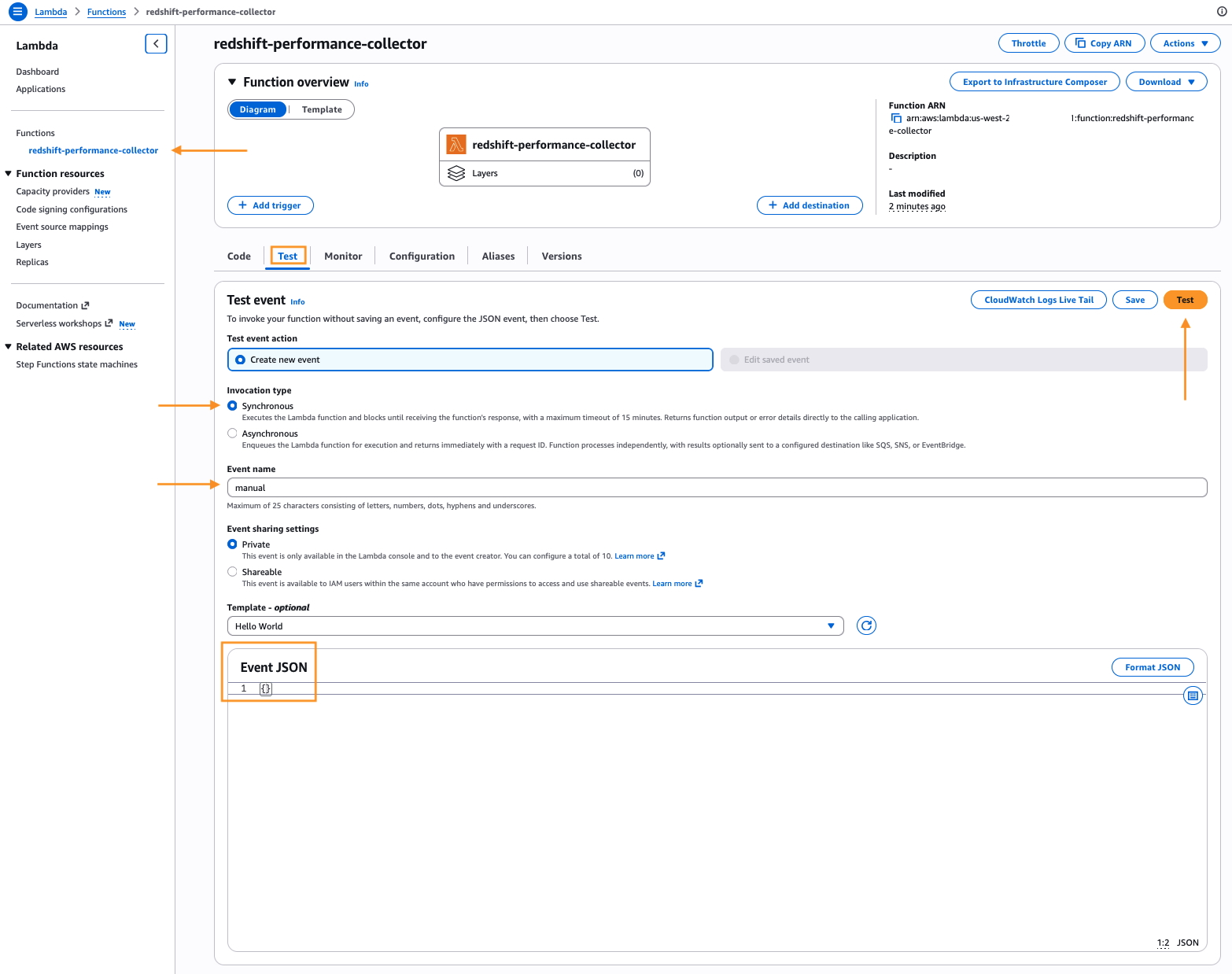
  • In the Lambda console, open the redshift-performance-collector function and choose Test. Create a test event named manual with the body {} and choose Test.

    Lambda console for “redshift-performance-collector,” Test tab. A new test event named “manual” is being configured with Invocation type set to Synchronous, event sharing set to Private, the “Hello World” template selected, and an empty {} Event JSON body. Annotation arrows point to the function in the left nav, the Synchronous option, the event name, the Event JSON field, and the Test button.

    Figure 9 – Test end-to-end workflow

  • The function completes in under a minute. Check the Monitor tab for the invocation log via the CloudWatch live logs link.
  • In the Amazon S3 console, open your bucket. Confirm that the telemetry/ prefix contains a JSON file with the current timestamp.
  • Within 2–4 minutes, the analyzer publishes a message to the SNS topic. Check the email address you subscribed for the summary with the top 10 recommendations. Confirm that the recommendations/ prefix in Amazon S3 contains the full JSON.
Each recommendation has a priority (critical, high, medium, low) and a category (query_optimization, table_design, capacity, wlm, maintenance, or ingestion). It also includes a signal_source that names the signals and CloudWatch metrics that triggered it, a plain-language explanation, a specific SQL or configuration action, and an expected impact estimate.
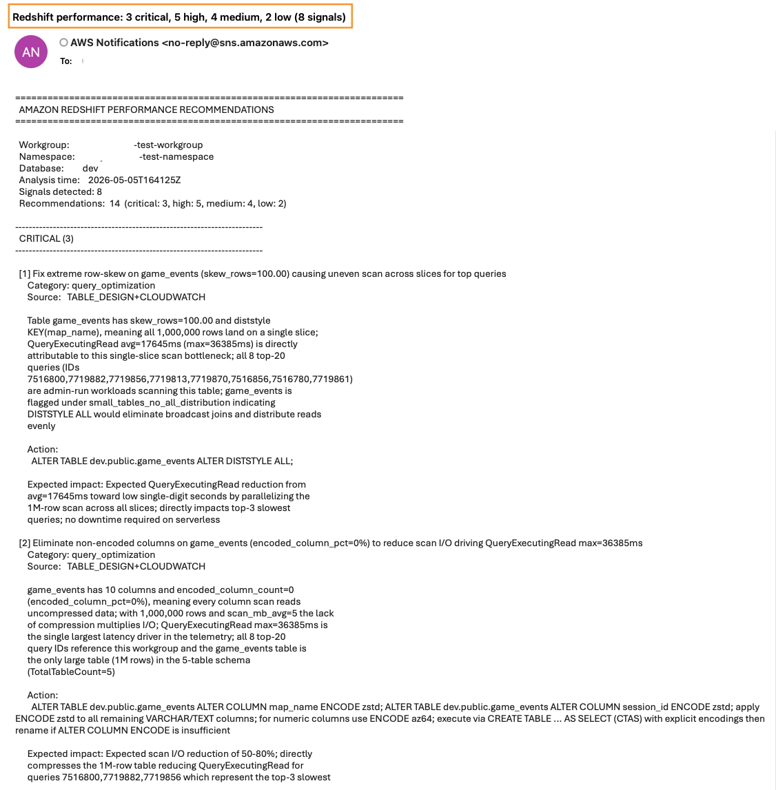
Email notification from AWS Notifications with the subject “Redshift performance: 3 critical, 5 high, 4 medium, 2 low (8 signals)” highlighted. The body is a plain-text “Amazon Redshift Performance Recommendations” report listing workgroup, namespace, database, analysis time, and 14 recommendations. Two critical items are shown for the game_events table: fixing extreme row-skew via DISTSTYLE ALL, and eliminating non-encoded columns with column compression, each with a category, source, explanation, SQL action, and expected impact.

Figure 10 – Sample analyzer emailed output

Best practices

  • Tune thresholds to your workload. The default thresholds in compute_signals() come from the Amazon Redshift operational review playbook. For high-velocity ingestion or small-cluster environments, consider lowering the small-insert threshold, widening the stale-statistics window, or adding custom signals for your own tables.
  • Keep the signal-to-metric correlations current. When you add a signal, also add a matching correlation in build_correlations(). The inline >> CORRELATION lines are what make the model connect an infrastructure metric to an application-level symptom.
  • Review recommendations before you act. The analyzer produces prioritized suggestions, but VACUUM, ANALYZE, and ALTER TABLE actions change table state. Read the explanation and action on each recommendation, validate the SQL against your schema, and run it during a maintenance window.

Cleaning up

To avoid ongoing charges, delete the resources you created for this solution:

  • The two AWS Lambda functions: redshift-performance-collector and redshift-performance-analyzer.
  • The Amazon EventBridge rule: redshift-performance-daily.
  • The Amazon SNS topic and its email subscription: redshift-performance-recommendations.
  • The Amazon S3 bucket, including the telemetry/ and recommendations/ objects.
  • The AWS Secrets Manager secret: redshift-performance-admin.
  • The IAM role and its inline policy: redshift-performance-recommendations-role.

Conclusion

You now have a daily performance review for Amazon Redshift Serverless that runs entirely on AWS Lambda, stores every run in Amazon S3, and delivers prioritized recommendations by email. The signal-based prompt pattern keeps the Amazon Bedrock cost low and the recommendations specific to your workload.

To learn more, see the following resources:


About the authors

Steve Phillips

Steve Phillips

Steve is a Principal Technical Account Manager and Analytics specialist at AWS in the North America region. Steve currently focuses on data warehouse architectural design, AI/ML data foundations, data lakes, data ingestion pipelines, and cloud distributed architectures.

Richard Raseley

Richard Raseley

Richard is a Senior Technical Account Manager in North America who works with Games customers. He is passionate about applying his background in automation, cloud computing, networking, and storage to help customers build AI solutions.

Build governance dashboards for Amazon SageMaker Catalog with Amazon Quick

Post Syndicated from Steve Phillips original https://aws.amazon.com/blogs/big-data/build-governance-dashboards-for-amazon-sagemaker-catalog-with-amazon-quick/

Maintaining visibility into your data catalog’s health requires more than ad-hoc queries. Data stewards and compliance teams need automated dashboards that surface governance metrics and alert them when issues arise. These issues include undocumented assets, missing ownership, and stale metadata.

In a previous post, we showed you how to query Amazon SageMaker Catalog metadata using SQL by using the metadata export feature. This post builds on that foundation by demonstrating how to create governance dashboards with Amazon Quick.

Amazon Quick is an agentic AI-powered digital workspace that provides integrated analytics, automation, and research capabilities. With Amazon Quick Sight, a component of Amazon Quick, you can create interactive dashboards and visualizations with automatic chart suggestions and machine learning (ML) insights.

We walk through how to connect Amazon Quick Sight to your Amazon SageMaker Catalog metadata and build governance dashboards using natural language prompts.

Solution overview

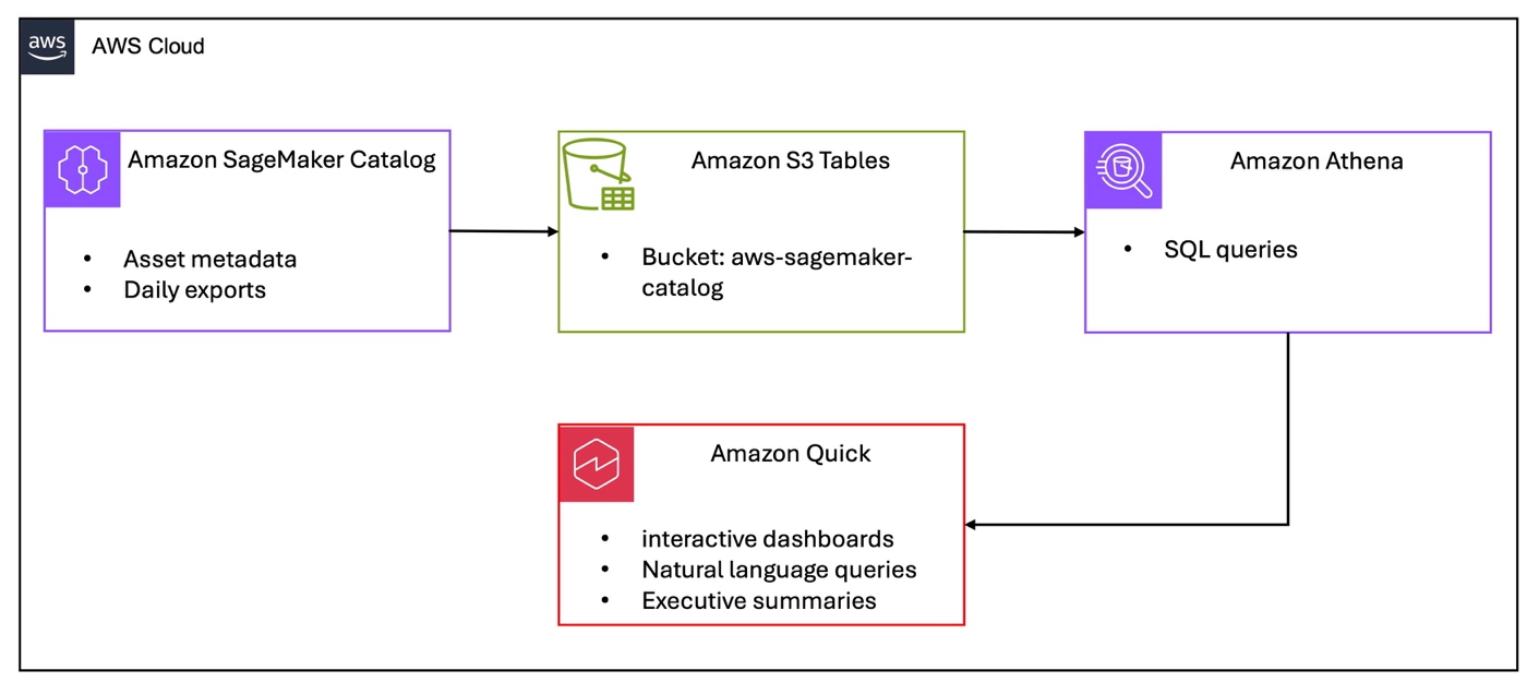
This solution extends the metadata export architecture by adding a visualization layer:

  1. Amazon SageMaker Catalog exports asset metadata daily to Amazon Simple Storage Service (Amazon S3) Tables
  2. Amazon Athena queries the metadata using standard SQL
  3. Amazon Quick Sight connects to Athena for interactive dashboards
  4. Amazon Quick uses natural language to build visualizations

AWS Cloud architecture diagram showing the data flow for SageMaker Catalog metadata visualization. Amazon SageMaker Catalog exports asset metadata and daily exports to Amazon S3 Tables in a bucket named aws-sagemaker-catalog. Amazon Athena queries the S3 Tables data using SQL queries. Amazon Quick connects to Athena to provide interactive dashboards, natural language queries, and executive summaries. Arrows indicate the left-to-right data flow from SageMaker Catalog to S3 Tables to Athena, with Athena connecting down to Amazon Quick.

Figure 1 – Amazon SageMaker Catalog governance dashboard architecture

Prerequisites

Before you begin, complete the following steps from Analyzing your data catalog: Query SageMaker Catalog metadata with SQL. You must also have the following:

  • Amazon SageMaker Catalog metadata export enabled
  • Amazon Athena configured with query results S3 bucket
  • AWS Lake Formation permissions configured for AWS Identity and Access Management (IAM)-based access
  • Verified that the asset_metadata.asset table contains data

Additionally, you need:

Building a governance dashboard with Amazon Quick Sight

To visualize catalog health metrics, connect Amazon Quick Sight to your Athena metadata tables.

Configure Amazon Quick Sight permissions

  1. Grant permissions to the Amazon Quick Sight service role.

The Amazon Quick Sight service role (default name: aws-quicksight-service-role-v0) needs permissions to access Amazon S3 Tables and AWS Glue catalog:

{
  "Version": "2012-10-17",
  "Statement": [
    {
      "Effect": "Allow",
      "Action": [
        "s3tables:GetTableBucket",
        "s3tables:GetTable",
        "s3tables:GetTableMetadataLocation"
      ],
      "Resource": "arn:aws:s3tables:REGION:ACCOUNT_ID:bucket/aws-sagemaker-catalog/*"
    },
    {
      "Effect": "Allow",
      "Action": "glue:GetCatalog",
      "Resource": "arn:aws:glue:REGION:ACCOUNT_ID:catalog"
    }
  ]
}

Add this as an inline policy to the Amazon Quick Sight service role in the IAM console.

  1. Grant AWS Lake Formation permissions:

Both the Amazon Quick Sight service role and your Amazon Quick Sight admin user need AWS Lake Formation permissions on the S3 Tables catalog. First, find your Amazon Quick Sight admin user ARN by running this AWS Command Line Interface (AWS CLI) command:

aws quicksight list-users \
  --aws-account-id ACCOUNT_ID \
  --namespace default \
  --region us-east-1

Amazon Quick Sight users are managed in the Amazon Quick Sight home AWS Region (us-east-1).To grant permissions, use the Lake Formation console.

  1. Navigate to AWS Lake Formation in the AWS Management Console.
  2. Select Data permissions and Grant.
  3. For Principals, choose SAML users and groups.
  4. Enter your Amazon Quick Sight admin user ARN (from the preceding command).
  5. Under LF-Tags or catalog resources, choose Named Data Catalog resources.
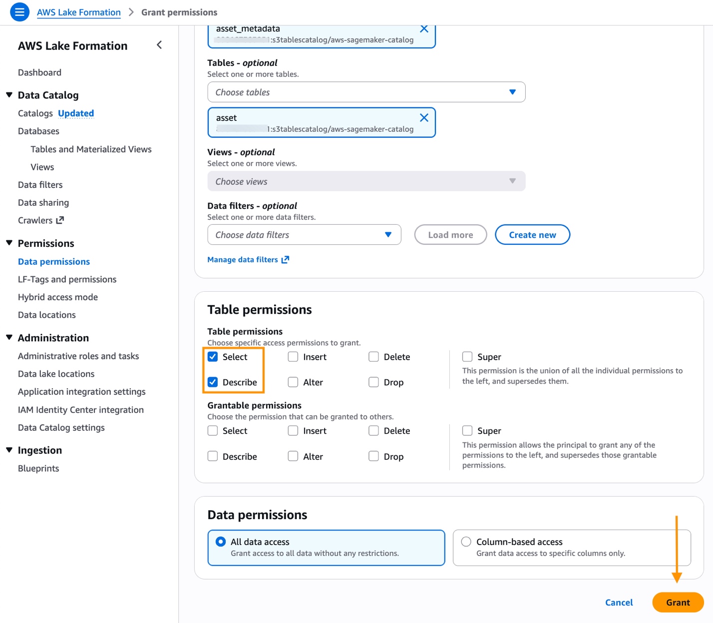
  6. For Catalogs, choose the S3 Tables catalog: ACCOUNT_ID:s3tablescatalog/aws-sagemaker-catalog.
  7. For Databases, choose asset_metadata.
  8. Under Tables, choose asset.
  9. For Table permissions, choose Select and Describe.
  10. Select Grant.

Screenshot of AWS Lake Formation Grant permissions page showing the complete permission configuration workflow. At the top, the resource selection shows the 'asset_metadata' database and 'asset' table from the s3tablescatalog/aws-sagemaker-catalog catalog. Below that are optional sections for Views and Data filters, both unselected. The main content area displays three permission configuration sections. First, the 'Table permissions' section shows two subsections: 'Table permissions' with checkboxes for Select (checked, highlighted with orange box), Describe (checked, highlighted with orange box), Insert, Alter, Delete, Drop, and Super; and 'Grantable permissions' with the same permission options all unchecked. The Super permission includes explanatory text stating it is the union of all individual permissions and supersedes them. The Grantable permissions section explains that this allows the principal to grant any of the permissions to others and supersedes grantable permissions. At the bottom, the 'Data permissions' section displays two radio button options: 'All data access' (selected) which grants access to all data without restrictions, and 'Column-based access' which grants data access to specific columns only. An orange arrow points from the right side down to the bottom right corner where 'Cancel' and 'Grant' buttons are located, with the Grant button highlighted in orange.

Figure 2 – Grant access to Amazon SageMaker Catalog resources

  1. Repeat steps 1–9 for the Amazon Quick Sight service role, but in step 2 choose IAM users and roles instead.

When choosing the catalog in the Lake Formation console, you must choose the full S3 Tables catalog identifier (ACCOUNT_ID:s3tablescatalog/aws-sagemaker-catalog) to see the asset_metadata database.

Create an Amazon Quick Sight dataset.

Access S3 Tables data by creating a Quick Sight dataset using an Amazon Athena data source and the custom SQL option. An S3 Tables data source is also available but requires additional permissions. See Introducing new data source with S3 Tables in Amazon Quick for using S3 Tables as an Amazon Quick data source.

  1. Open Amazon Quick Sight in the AWS Management Console.
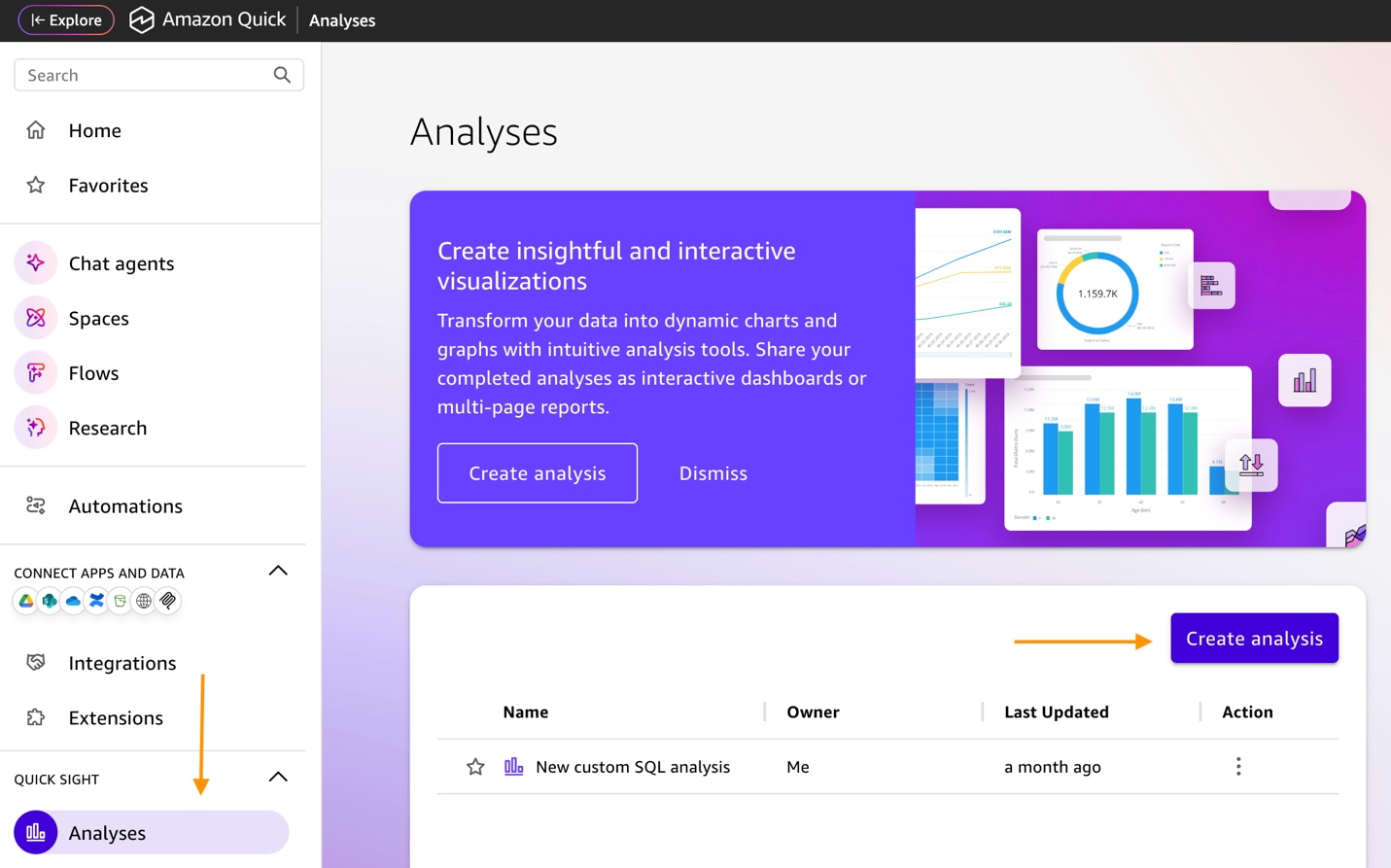
  2. Select Analyses and Create analysis.

Amazon QuickSight Analyses page showing the left navigation menu with Analyses selected under the Quick Sight section. The main content area displays a promotional banner for creating insightful and interactive visualizations with sample chart previews. Below the banner, an orange arrow points to the Create analysis button in the upper right. A table lists an existing analysis named New custom SQL analysis owned by Me and last updated a month ago.

Figure 3 – Create Amazon Quick Sight analysis

  1. Choose Create dataset and Create data source.

Amazon QuickSight Create Analysis dialog prompting the user to choose a dataset. A search field for datasets is shown at the top left. An orange arrow points to the Create dataset button in the upper right. A table below lists one available dataset named New custom SQL with a data source of New custom SQL, owned by Me, and last modified on March 5, 2026.

Figure 4 – Create dataset

  1. Select Amazon Athena as the data source and select Next.
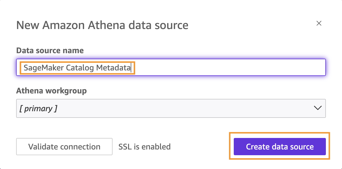
  2. Enter a Data source name (for example, “SageMaker Catalog Metadata”) and choose Create data source.

Amazon QuickSight New Amazon Athena data source configuration dialog. The Data source name field is highlighted with an orange box and contains the value SageMaker Catalog Metadata. The Athena workgroup dropdown is set to primary. A Validate connection button and SSL is enabled label appear at the bottom left. An orange box highlights the Create data source button at the bottom right.

Figure 5 – Create data source

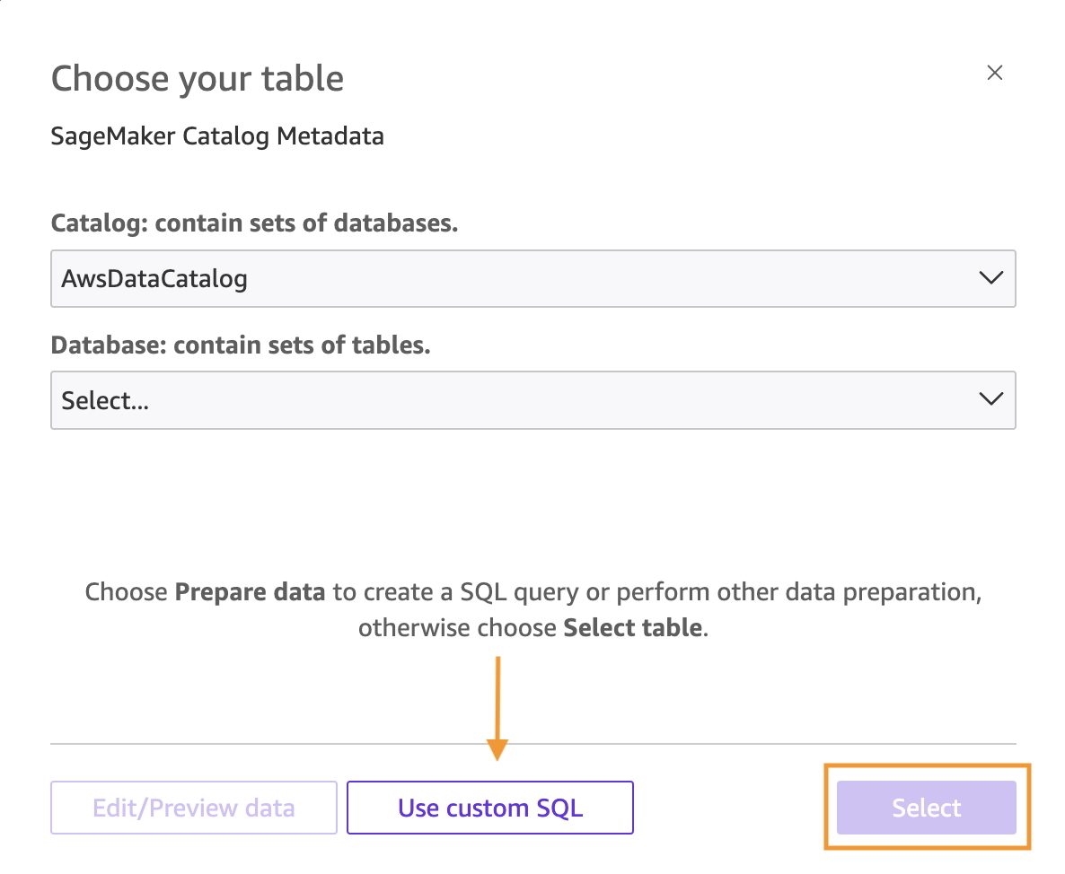
  1. Select Use custom SQL and enter a custom SQL query that references the S3 Tables catalog using the full three-part name.

Amazon QuickSight Choose your table dialog for the SageMaker Catalog Metadata data source. The Catalog dropdown is set to AwsDataCatalog and the Database dropdown shows a Select prompt. An instructional message explains to choose Prepare data to create a SQL query or choose Select table. An orange arrow points down to the Use custom SQL button highlighted with a blue box at the bottom center. The Select button is highlighted with an orange box at the bottom right.

Figure 6 – Use custom SQL

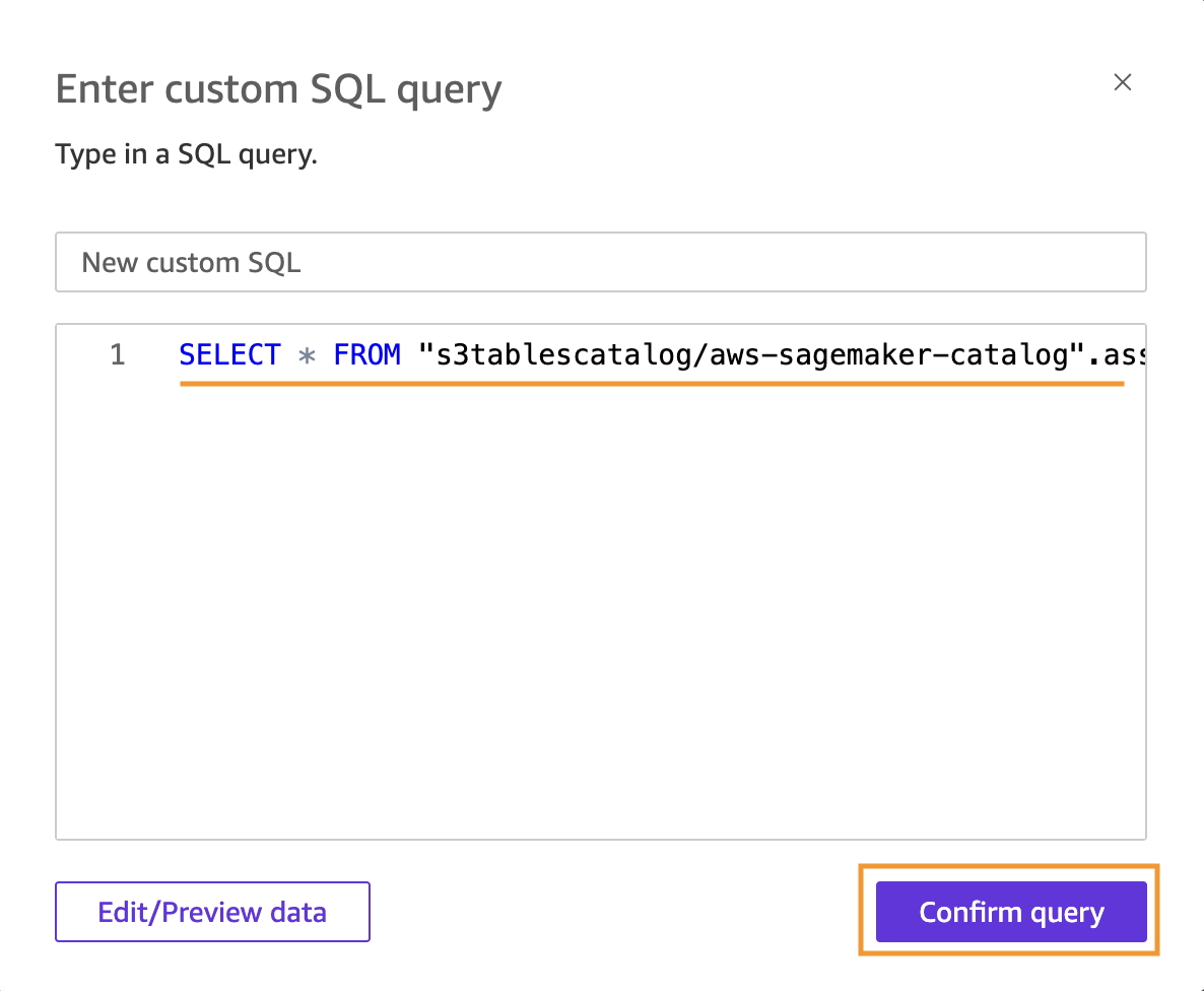
Amazon QuickSight Enter custom SQL query dialog. The query name field shows New custom SQL. The SQL editor contains a query reading SELECT FROM s3tablescatalog/aws-sagemaker-catalog with the query text underlined in orange. An orange box highlights the Confirm query button at the bottom right. An Edit/Preview data button appears at the bottom left.

Figure 7 – Enter custom SQL

SELECT * FROM "s3tablescatalog/aws-sagemaker-catalog".asset_metadata.asset

  1. Select Confirm query.
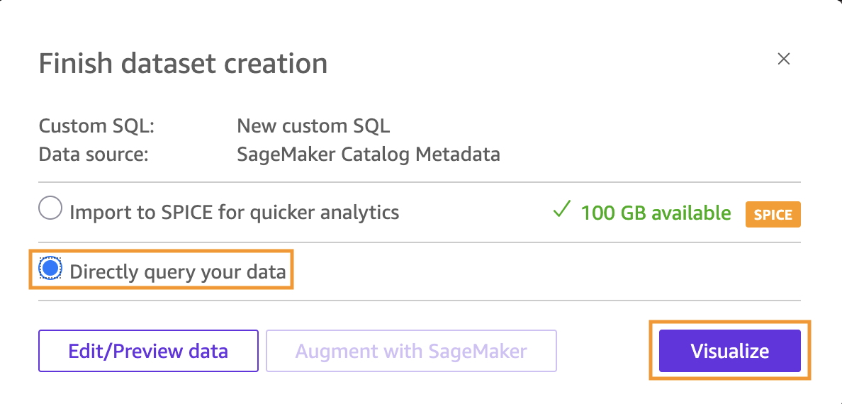
  2. Choose Directly query your data (SPICE import may fail with S3 Tables catalogs)
    Amazon QuickSight Finish dataset creation dialog showing the custom SQL dataset named New custom SQL with the SageMaker Catalog Metadata data source. Two radio button options are displayed: Import to SPICE for quicker analytics with 100 GB available shown in green, and Directly query your data which is selected and highlighted with an orange box. An orange box highlights the Visualize button at the bottom right. Edit/Preview data and Augment with SageMaker buttons appear at the bottom left and center.

Figure 8 – Directly query your data

  1. Choose Visualize and Create to start building your dashboard.

Create visualizations with Amazon Quick.

With Amazon Quick, you can build governance dashboards using natural language prompts. This removes the need for manual field configuration. This approach is faster and more intuitive than traditional dashboard building.The Amazon Quick Sight user must have AdminPro or AuthorPro subscription (the Build feature isn’t available for Reader users).Start building your dashboard with the following steps:

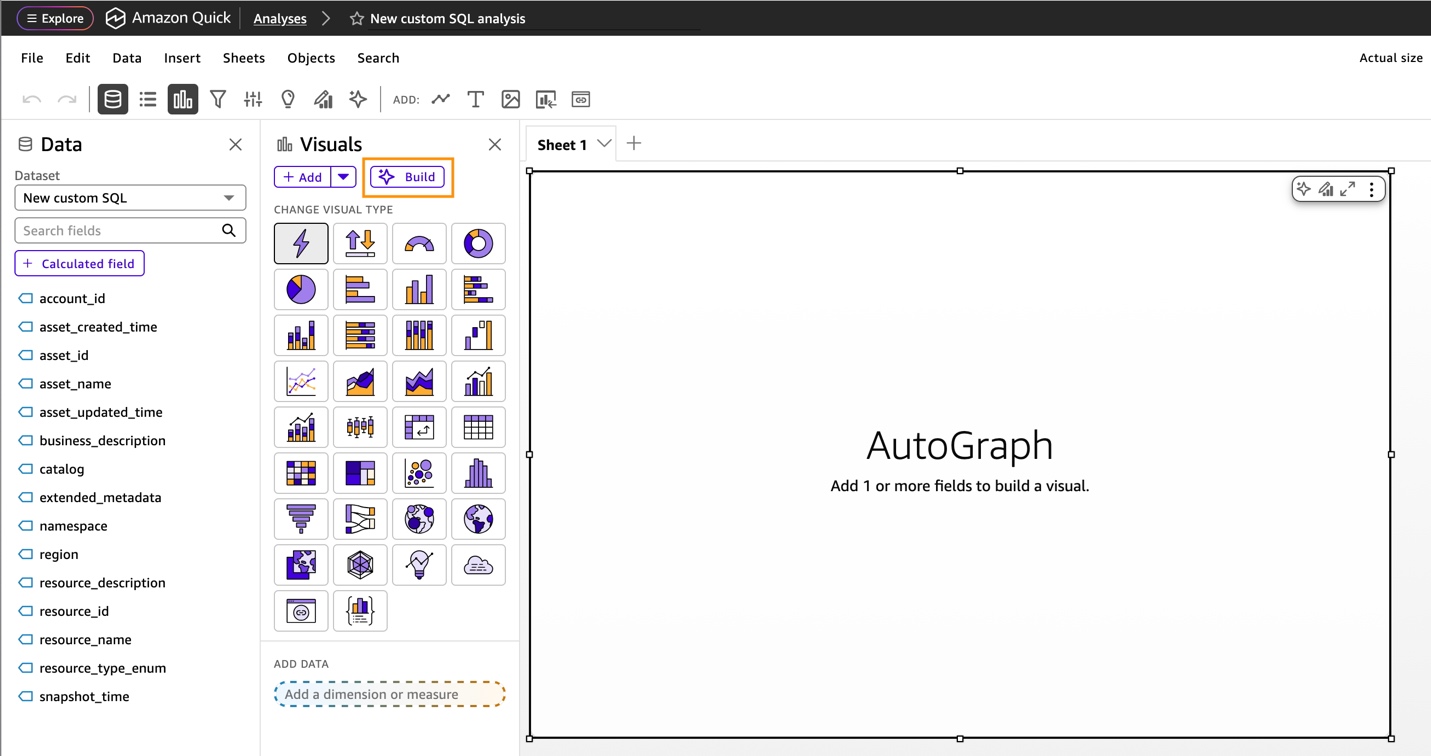
  1. Select Build in the top toolbar to open the natural language builder.

Amazon QuickSight analysis editor for New custom SQL analysis. The left Data panel shows the dataset fields including accountid, asset_created_time, asset_id, asset_name, asset_updated_time, business_description, catalog, extended_metadata, namespace, region, resource_description, resource_id, resource_name, resource_type_enum, and snapshot_time. The center Visuals panel shows the Build button highlighted with an orange box and a grid of available chart types. The right canvas area displays an empty AutoGraph placeholder with the message Add 1 or more fields to build a visual. An Add Data section with a dashed border prompts to add a dimension or measure.

Figure 9 – Amazon Quick build dashboard

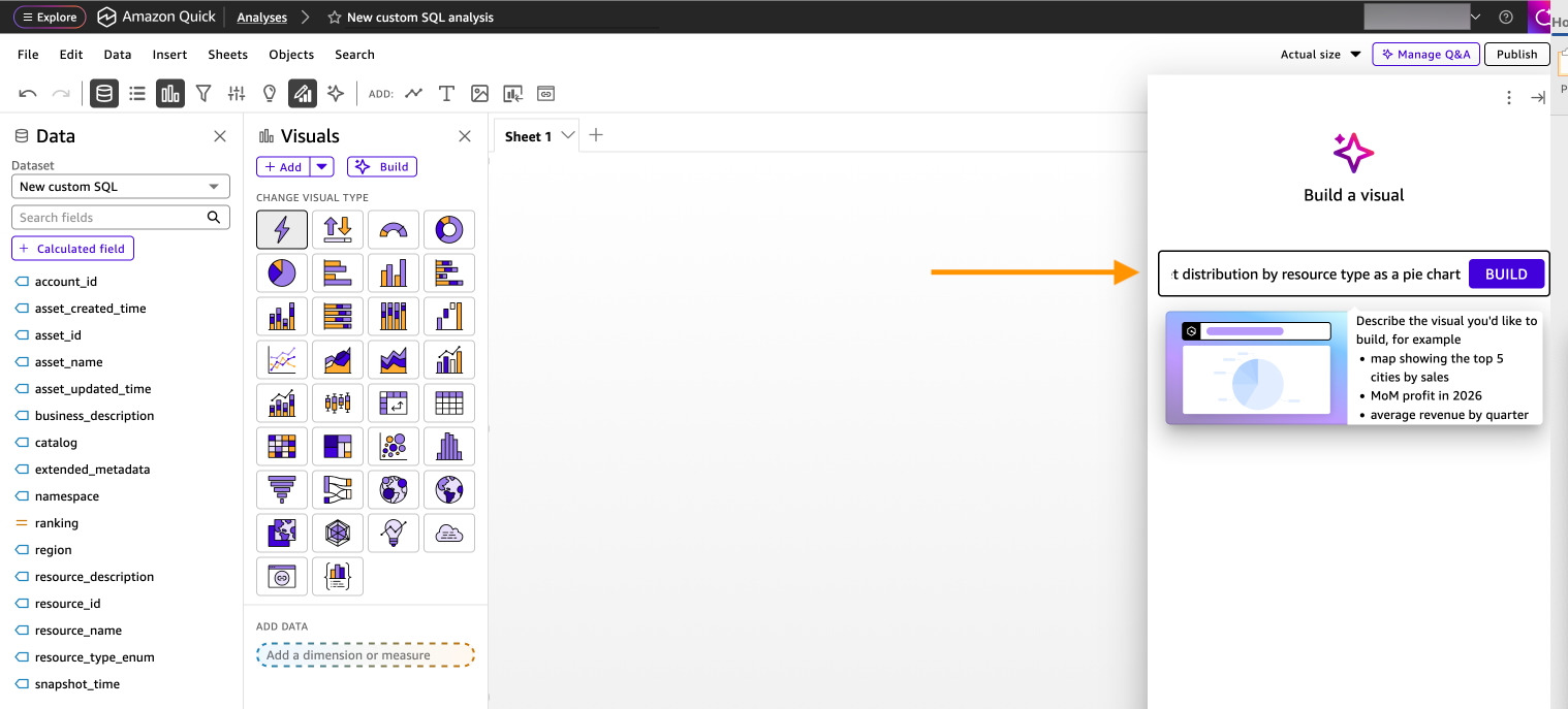
  1. You will see a text box where you can describe the visualization that you want to create.

Amazon QuickSight analysis editor with the Build a visual panel open on the right side. An orange arrow points to the natural language input field where the user has typed a prompt requesting asset distribution by resource type as a pie chart, with a Build button next to it. Below the input field, a tooltip explains to describe the visual you would like to build with examples including map showing the top 5 cities by sales, MoM profit in 2026, and average revenue by quarter. The left Data panel shows dataset fields and the center Visuals panel displays available chart types.

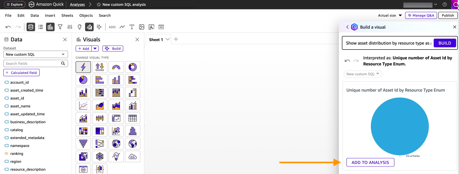
Create each visualization using natural language. For each of the six recommended visualizations, enter the corresponding natural language prompt, select Build, then choose ADD TO ANALYSIS.

Amazon QuickSight analysis editor with the Build a visual panel open on the right side. The natural language prompt reads Show asset distribution by resource type as a pie chart with a Build button. Below, the system shows the interpretation as Unique number of Asset Id by Resource Type Enum using the New custom SQL dataset. A pie chart preview is displayed showing the distribution with a large segment labeled GlueTable. An orange arrow points to the Add to Analysis button at the bottom of the panel.

Figure 11 – Add to analysis

Visualization 1: Asset inventory by type

Show count of asset_id by resource_type_enum as a pie chart

After the pie chart is created, choose ADD TO ANALYSIS.

Visualization 2: Documentation completeness

Show count of asset_id where business_description is not null asa KPI

After the KPI is created, choose ADD TO ANALYSIS.

Visualization 3: Monthly registration trends

Show count of asset_id by asset_created_time month as a line chart

After the line chart is created, choose ADD TO ANALYSIS.

Visualization 4: Asset count by account

Show count of asset_id by account_id as a bar chart

After the bar chart is created, choose ADD TO ANALYSIS.

Visualization 5: Namespace distribution

Show count of asset_id by namespace as a treemap

After the treemap is created, choose ADD TO ANALYSIS.

Visualization 6: Resource type by namespace

Show count of asset_id by resource_type_enum and namespace as a heat map

Choose ADD TO ANALYSIS

  1. Arrange and publish your governance dashboard with the following steps:
  2. Delete any empty or unwanted visualizations by choosing the three dots menu and choosing Delete.
  3. Arrange visualizations by dragging them into your preferred layout.
  4. Resize visualizations to emphasize key metrics.
  5. Add titles to each visualization for clarity.
  6. Choose PUBLISH in the top right corner.
  7. Enter a dashboard name: “SageMaker Catalog Governance Dashboard”.
  8. Verify these options are selected:
    1. Allow executive summary.
    2. Allow sharing stories.
    3. Allow sharing scenarios.
  9. Choose Publish dashboard.

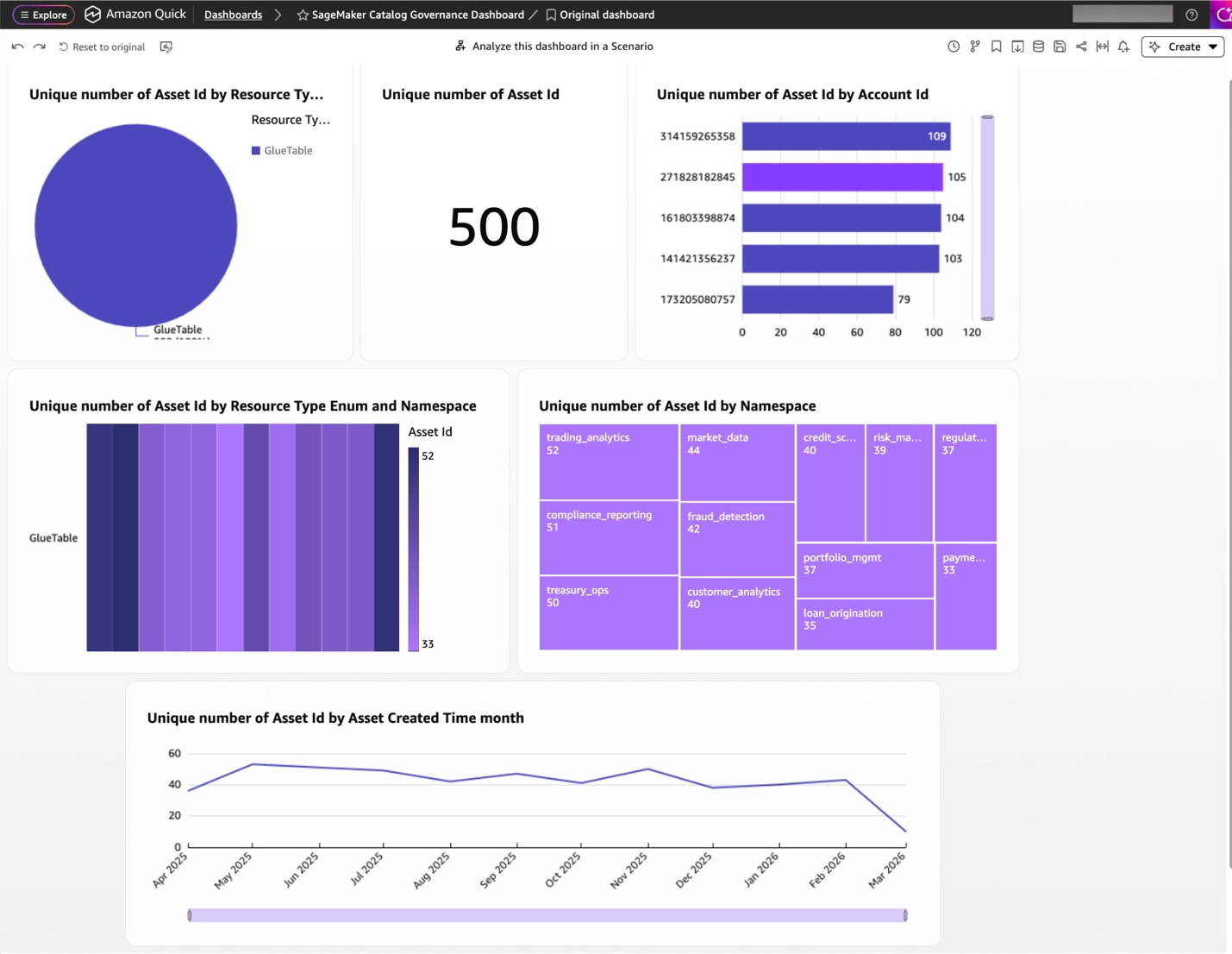
Amazon QuickSight SageMaker Catalog Governance Dashboard showing five visualizations. Top left is a pie chart titled Unique number of Asset Id by Resource Type showing all assets as GlueTable type. Top center is a key performance indicator displaying a total of 500 unique assets. Top right is a horizontal bar chart titled Unique number of Asset Id by Account Id showing five AWS account IDs with values of 109, 105, 104, 103, and 79 assets respectively. Middle left is a stacked bar chart titled Unique number of Asset Id by Resource Type Enum and Namespace showing GlueTable assets distributed across namespaces with values ranging from 33 to 52. Middle right is a treemap titled Unique number of Asset Id by Namespace with trading_analytics at 52, compliance_reporting at 51, treasury_ops at 50, market_data at 44, fraud_detection at 42, customer_analytics at 40, credit_scoring at 40, risk_management at 39, portfolio_mgmt at 37, regulatory at 37, loan_origination at 35, and payments at 33. Bottom is a line chart titled Unique number of Asset Id by Asset Created Time month showing asset creation trends from April 2025 through March 2026 with values fluctuating between approximately 30 and 50 assets per month.

Figure 12 – Amazon SageMaker Catalog governance dashboard

    1. Analyze your dashboard with natural language.

After you publish, you can ask questions about your governance data:

    1. On the dashboard, choose Analyze this dashboard in a Scenario in the top center.
    2. In the Data to Insights panel, enter natural language questions such as:
      1. “Which resource types have the lowest documentation rates?”
      2. “How many assets were registered last month compared to this month?”
      3. “What percentage of assets lack ownership information?”
    3. Choose Submit to generate AI-powered insights.

Amazon Quick analyzes your data and provides insights with supporting visualizations.

    1. Generate executive summaries

Create automated governance reports for data stewards and compliance teams:

    1. Choose the Amazon Quick logo in the top left to return to the home page
    2. Select Dashboards from the left panel
    3. Choose your “SageMaker Catalog Governance Dashboard”
    4. Choose the Create dropdown menu in the top right
    5. Select Executive Summary

Amazon Quick will automatically generate a summary with key governance insights, including Total asset counts and growth trends, Documentation completeness metrics, Ownership coverage statistics, and Classification distribution analysis.

    1. Create governance stories.

Build governance reports that combine multiple dashboards:

    1. From the Create dropdown, select Story.
    2. Enter a prompt: “Write a summary of catalog governance metrics and data quality trends”.
    3. Choose Add to select dashboards to include in the report.
    4. Choose Build (this might take a few minutes to complete).

Amazon Quick will generate a narrative report combining your visualizations with AI-generated insights. Share the reports with leadership or compliance teams.

Governance dashboards contain metadata such as ownership and classification details. Restrict access to users who need it. In the Amazon Quick Sight console, open the dashboard, choose Share, and grant access to named users or a dedicated Quick Sight group (for example, data-stewards) instead of selecting Everyone in this account. Review the dashboard’s permissions periodically and remove entries that are no longer needed.

Cleaning up

To avoid ongoing charges, clean up the resources created in this walkthrough. Delete Amazon Quick Sight resources including the dashboard, analyses, and dataset.

Conclusion

In this post, you connected Amazon Quick Sight to your Amazon SageMaker Catalog metadata export, built governance dashboards using the Amazon Quick natural language prompts. This approach gives data stewards and compliance teams visibility into catalog health through six key visualizations covering asset inventory, documentation completeness, registration trends, account distribution, classification coverage, and stale asset detection.

Together with the metadata export and SQL query capabilities covered in the Analyzing your data catalog: Query SageMaker Catalog metadata with SQL post, this solution provides a complete, low-overhead governance monitoring pipeline from raw catalog metadata to executive-ready.

To learn more about Amazon SageMaker Catalogs, see Amazon SageMaker Catalog documentation. To expand the work done with Amazon Quick, review Amazon Quick Sight documentation.


About the authors

Steve Phillips

Steve is a Principal Technical Account Manager and Analytics specialist at AWS in the North America region. Steve currently focuses on data warehouse architectural design, data lakes, data ingestion pipelines, and cloud distributed architectures.

Ramesh Singh

Ramesh is a Senior Product Manager Technical (External Services) at AWS in Seattle, Washington, currently with the Amazon SageMaker team. He is passionate about building high-performance ML/AI and analytics products that help enterprise customers achieve their critical goals using cutting-edge technology.

Pradeep Misra

Pradeep is a Principal Analytics and Applied AI Solutions Architect at AWS. He is passionate about solving customer challenges using data, analytics, and Applied AI. Outside of work, he likes exploring new places and playing badminton with his family. He also likes doing science experiments, building LEGOs, and watching anime with his daughters.

Rohith Kayathi

Rohith is a Senior Software Engineer at Amazon Web Services (AWS) working with Amazon SageMaker team. He leads business data catalog, generative AI–powered metadata curation, and lineage solutions. He is passionate about building large-scale distributed systems, solving complex problems, and setting the bar for engineering excellence for his team.

Amazon Redshift data ingestion options

Post Syndicated from Steve Phillips original https://aws.amazon.com/blogs/big-data/amazon-redshift-data-ingestion-options/

Amazon Redshift, a warehousing service, offers a variety of options for ingesting data from diverse sources into its high-performance, scalable environment. Whether your data resides in operational databases, data lakes, on-premises systems, Amazon Elastic Compute Cloud (Amazon EC2), or other AWS services, Amazon Redshift provides multiple ingestion methods to meet your specific needs. The currently available choices include:

This post explores each option (as illustrated in the following figure), determines which are suitable for different use cases, and discusses how and why to select a specific Amazon Redshift tool or feature for data ingestion.

A box indicating Amazon Redshift in the center of the image with boxes from right to left for Amazon RDS MySQL and PostgreSQL, Amazon Aurora MySQL and PostreSQL, Amazon EMR, Amazon Glue, Amazon S3 bucket, Amazon Managed Streaming for Apache Kafka and Amazon Kinesis. Each box has an arrow pointing to Amazon Redshift. Each arrow has the following labels: Amazon RDS & Amazon Aurora: zero-ETL and federated queries; AWS Glue and Amazon EMR: spark connector; Amazon S3 bucket: COPY command; Amazon Managed Streaming for Apache Kafka and Amazon Kinesis: redshift streaming. Amazon Data Firehose has an arrow pointing to Amazon S3 bucket indicating the data flow direction.

Amazon Redshift COPY command

The Redshift COPY command, a simple low-code data ingestion tool, loads data into Amazon Redshift from Amazon S3, DynamoDB, Amazon EMR, and remote hosts over SSH. It’s a fast and efficient way to load large datasets into Amazon Redshift. It uses massively parallel processing (MPP) architecture in Amazon Redshift to read and load large amounts of data in parallel from files or data from supported data sources. This allows you to utilize parallel processing by splitting data into multiple files, especially when the files are compressed.

Recommended use cases for the COPY command include loading large datasets and data from supported data sources. COPY automatically splits large uncompressed delimited text files into smaller scan ranges to utilize the parallelism of Amazon Redshift provisioned clusters and serverless workgroups. With auto-copy, automation enhances the COPY command by adding jobs for automatic ingestion of data.

COPY command advantages:

  • Performance – Efficiently loads large datasets from Amazon S3 or other sources in parallel with optimized throughput
  • Simplicity – Straightforward and user-friendly, requiring minimal setup
  • Cost-optimized – Uses Amazon Redshift MPP at a lower cost by reducing data transfer time
  • Flexibility – Supports file formats such as CSV, JSON, Parquet, ORC, and AVRO

Amazon Redshift federated queries

Amazon Redshift federated queries allow you to incorporate live data from Amazon RDS or Aurora operational databases as part of business intelligence (BI) and reporting applications.

Federated queries are useful for use cases where organizations want to combine data from their operational systems with data stored in Amazon Redshift. Federated queries allow querying data across Amazon RDS for MySQL and PostgreSQL data sources without the need for extract, transform, and load (ETL) pipelines. If storing operational data in a data warehouse is a requirement, synchronization of tables between operational data stores and Amazon Redshift tables is supported. In scenarios where data transformation is required, you can use Redshift stored procedures to modify data in Redshift tables.

Federated queries key features:

  • Real-time access – Enables querying of live data across discrete sources, such as Amazon RDS and Aurora, without the need to move the data
  • Unified data view – Provides a single view of data across multiple databases, simplifying data analysis and reporting
  • Cost savings – Eliminates the need for ETL processes to move data into Amazon Redshift, saving on storage and compute costs
  • Flexibility – Supports Amazon RDS and Aurora data sources, offering flexibility in accessing and analyzing distributed data

Amazon Redshift Zero-ETL integration

Aurora zero-ETL integration with Amazon Redshift allows access to operational data from Amazon Aurora MySQL-Compatible (and Amazon Aurora PostgreSQL-Compatible Edition, Amazon RDS for MySQL in preview), and DynamoDB from Amazon Redshift without the need for ETL in near real time. You can use zero-ETL to simplify ingestion pipelines for performing change data capture (CDC) from an Aurora database to Amazon Redshift. Built on the integration of Amazon Redshift and Aurora storage layers, zero-ETL boasts simple setup, data filtering, automated observability, auto-recovery, and integration with either Amazon Redshift provisioned clusters or Amazon Redshift Serverless workgroups.

Zero-ETL integration benefits:

  • Seamless integration – Automatically integrates and synchronizes data between operational databases and Amazon Redshift without the need for custom ETL processes
  • Near real-time insights – Provides near real-time data updates, so the most current data is available for analysis
  • Ease of use – Simplifies data architecture by eliminating the need for separate ETL tools and processes
  • Efficiency – Minimizes data latency and provides data consistency across systems, enhancing overall data accuracy and reliability

Amazon Redshift integration for Apache Spark

The Amazon Redshift integration for Apache Spark, automatically included through Amazon EMR or AWS Glue, provides performance and security optimizations when compared to the community-provided connector. The integration enhances and simplifies security with AWS Identity and Access Management (IAM) authentication support. AWS Glue 4.0 provides a visual ETL tool for authoring jobs to read from and write to Amazon Redshift, using the Redshift Spark connector for connectivity. This simplifies the process of building ETL pipelines to Amazon Redshift. The Spark connector allows use of Spark applications to process and transform data before loading into Amazon Redshift. The integration minimizes the manual process of setting up a Spark connector and shortens the time needed to prepare for analytics and machine learning (ML) tasks. It allows you to specify the connection to a data warehouse and start working with Amazon Redshift data from your Apache Spark-based applications within minutes.

The integration provides pushdown capabilities for sort, aggregate, limit, join, and scalar function operations to optimize performance by moving only the relevant data from Amazon Redshift to the consuming Apache Spark application. Spark jobs are suitable for data processing pipelines and when you need to use Spark’s advanced data transformation capabilities.

With the Amazon Redshift integration for Apache Spark, you can simplify the building of ETL pipelines with data transformation requirements. It offers the following benefits:

  • High performance – Uses the distributed computing power of Apache Spark for large-scale data processing and analysis
  • Scalability – Effortlessly scales to handle massive datasets by distributing computation across multiple nodes
  • Flexibility – Supports a wide range of data sources and formats, providing versatility in data processing tasks
  • Interoperability – Seamlessly integrates with Amazon Redshift for efficient data transfer and queries

Amazon Redshift streaming ingestion

The key benefit of Amazon Redshift streaming ingestion is the ability to ingest hundreds of megabytes of data per second directly from streaming sources into Amazon Redshift with very low latency, supporting real-time analytics and insights. Supporting streams from Kinesis Data Streams, Amazon MSK, and Data Firehose, streaming ingestion requires no data staging, supports flexible schemas, and is configured with SQL. Streaming ingestion powers real-time dashboards and operational analytics by directly ingesting data into Amazon Redshift materialized views.

Amazon Redshift streaming ingestion unlocks near real-time streaming analytics with:

  • Low latency – Ingests streaming data in near real time, making streaming ingestion ideal for time-sensitive applications such as Internet of Things (IoT), financial transactions, and clickstream analysis
  • Scalability – Manages high throughput and large volumes of streaming data from sources such as Kinesis Data Streams, Amazon MSK, and Data Firehose
  • Integration – Integrates with other AWS services to build end-to-end streaming data pipelines
  • Continuous updates – Keeps data in Amazon Redshift continuously updated with the latest information from the data streams

Amazon Redshift ingestion use cases and examples

In this section, we discuss the details of different Amazon Redshift ingestion use cases and provide examples.

Redshift COPY use case: Application log data ingestion and analysis

Ingesting application log data stored in Amazon S3 is a common use case for the Redshift COPY command. Data engineers in an organization need to analyze application log data to gain insights into user behavior, identify potential issues, and optimize a platform’s performance. To achieve this, data engineers ingest log data in parallel from multiple files stored in S3 buckets into Redshift tables. This parallelization uses the Amazon Redshift MPP architecture, allowing for faster data ingestion compared to other ingestion methods.

The following code is an example of the COPY command loading data from a set of CSV files in an S3 bucket into a Redshift table:

COPY myschema.mytable
FROM 's3://my-bucket/data/files/'
IAM_ROLE ‘arn:aws:iam::1234567891011:role/MyRedshiftRole’
FORMAT AS CSV;

This code uses the following parameters:

  • mytable is the target Redshift table for data load
  • s3://my-bucket/data/files/‘ is the S3 path where the CSV files are located
  • IAM_ROLE specifies the IAM role required to access the S3 bucket
  • FORMAT AS CSV specifies that the data files are in CSV format

In addition to Amazon S3, the COPY command loads data from other sources, such as DynamoDB, Amazon EMR, remote hosts through SSH, or other Redshift databases. The COPY command provides options to specify data formats, delimiters, compression, and other parameters to handle different data sources and formats.

To get started with the COPY command, see Using the COPY command to load from Amazon S3.

Federated queries use case: Integrated reporting and analytics for a retail company

For this use case, a retail company has an operational database running on Amazon RDS for PostgreSQL, which stores real-time sales transactions, inventory levels, and customer information data. Additionally, a data warehouse runs on Amazon Redshift storing historical data for reporting and analytics purposes. To create an integrated reporting solution that combines real-time operational data with historical data in the data warehouse, without the need for multi-step ETL processes, complete the following steps:

  1. Set up network connectivity. Make sure your Redshift cluster and RDS for PostgreSQL instance are in the same virtual private cloud (VPC) or have network connectivity established through VPC peering, AWS PrivateLink, or AWS Transit Gateway.
  2. Create a secret and IAM role for federated queries:
    1. In AWS Secrets Manager, create a new secret to store the credentials (user name and password) for your Amazon RDS for PostgreSQL instance.
    2. Create an IAM role with permissions to access the Secrets Manager secret and the Amazon RDS for PostgreSQL instance.
    3. Associate the IAM role with your Amazon Redshift cluster.
  3. Create an external schema in Amazon Redshift:
    1. Connect to your Redshift cluster using a SQL client or the query editor v2 on the Amazon Redshift console.
    2. Create an external schema that references your Amazon RDS for PostgreSQL instance:
CREATE EXTERNAL SCHEMA postgres_schema
FROM POSTGRES
DATABASE 'mydatabase'
SCHEMA 'public'
URI 'endpoint-for-your-rds-instance.aws-region.rds.amazonaws.com:5432'
IAM_ROLE 'arn:aws:iam::123456789012:role/RedshiftRoleForRDS'
SECRET_ARN 'arn:aws:secretsmanager:aws-region:123456789012:secret:my-rds-secret-abc123';
  1. Query tables in your Amazon RDS for PostgreSQL instance directly from Amazon Redshift using federated queries:
SELECT
    r.order_id,
    r.order_date,
    r.customer_name,
    r.total_amount,
    h.product_name,
    h.category
FROM
    postgres_schema.orders r
    JOIN redshift_schema.product_history h ON r.product_id = h.product_id
WHERE
    r.order_date >= '2024-01-01';
  1. Create views or materialized views in Amazon Redshift that combine the operational data from federated queries with the historical data in Amazon Redshift for reporting purposes:
CREATE MATERIALIZED VIEW sales_report AS
SELECT
    r.order_id,
    r.order_date,
    r.customer_name,
    r.total_amount,
    h.product_name,
    h.category,
    h.historical_sales
FROM
    (
        SELECT
            order_id,
            order_date,
            customer_name,
            total_amount,
            product_id
        FROM
            postgres_schema.orders
    ) r
    JOIN redshift_schema.product_history h ON r.product_id = h.product_id;

With this implementation, federated queries in Amazon Redshift integrate real-time operational data from Amazon RDS for PostgreSQL instances with historical data in a Redshift data warehouse. This approach eliminates the need for multi-step ETL processes and enables you to create comprehensive reports and analytics that combine data from multiple sources.

To get started with Amazon Redshift federated query ingestion, see Querying data with federated queries in Amazon Redshift.

Zero-ETL integration use case: Near real-time analytics for an ecommerce application

Suppose an ecommerce application built on Aurora MySQL-Compatible manages online orders, customer data, and product catalogs. To perform near real-time analytics with data filtering on transactional data to gain insights into customer behavior, sales trends, and inventory management without the overhead of building and maintaining multi-step ETL pipelines, you can use zero-ETL integrations for Amazon Redshift. Complete the following steps:

  1. Set up an Aurora MySQL cluster (must be running Aurora MySQL version 3.05-compatible with MySQL 8.0.32 or higher):
    1. Create an Aurora MySQL cluster in your desired AWS Region.
    2. Configure the cluster settings, such as the instance type, storage, and backup options.
  2. Create a zero-ETL integration with Amazon Redshift:
    1. On the Amazon RDS console, navigate to the Zero-ETL integrations
    2. Choose Create integration and select your Aurora MySQL cluster as the source.
    3. Choose an existing Redshift cluster or create a new cluster as the target.
    4. Provide a name for the integration and review the settings.
    5. Choose Create integration to initiate the zero-ETL integration process.
  3. Verify the integration status:
    1. After the integration is created, monitor the status on the Amazon RDS console or by querying the SVV_INTEGRATION and SYS_INTEGRATION_ACTIVITY system views in Amazon Redshift.
    2. Wait for the integration to reach the Active state, indicating that data is being replicated from Aurora to Amazon Redshift.
  4. Create analytics views:
    1. Connect to your Redshift cluster using a SQL client or the query editor v2 on the Amazon Redshift console.
    2. Create views or materialized views that combine and transform the replicated data from Aurora for your analytics use cases:
CREATE MATERIALIZED VIEW orders_summary AS
SELECT
    o.order_id,
    o.customer_id,
    SUM(oi.quantity * oi.price) AS total_revenue,
    MAX(o.order_date) AS latest_order_date
FROM
    aurora_schema.orders o
    JOIN aurora_schema.order_items oi ON o.order_id = oi.order_id
GROUP BY
    o.order_id,
    o.customer_id;
  1. Query the views or materialized views in Amazon Redshift to perform near real-time analytics on the transactional data from your Aurora MySQL cluster:
SELECT
	customer_id,
	SUM(total_revenue) AS total_customer_revenue,
	MAX(latest_order_date) AS most_recent_order
FROM
	orders_summary
GROUP BY
	customer_id
ORDER BY
	total_customer_revenue DESC;

This implementation achieves near real-time analytics for an ecommerce application’s transactional data using the zero-ETL integration between Aurora MySQL-Compatible and Amazon Redshift. The data automatically replicates from Aurora to Amazon Redshift, eliminating the need for multi-step ETL pipelines and supporting insights from the latest data quickly.

To get started with Amazon Redshift zero-ETL integrations, see Working with zero-ETL integrations. To learn more about Aurora zero-ETL integrations with Amazon Redshift, see Amazon Aurora zero-ETL integrations with Amazon Redshift.

Integration for Apache Spark use case: Gaming player events written to Amazon S3

Consider a large volume of gaming player events stored in Amazon S3. The events require data transformation, cleansing, and preprocessing to extract insights, generate reports, or build ML models. In this case, you can use the scalability and processing power of Amazon EMR to perform the required data changes using Apache Spark. After it’s processed, the transformed data must be loaded into Amazon Redshift for further analysis, reporting, and integration with BI tools.

In this scenario, you can use the Amazon Redshift integration for Apache Spark to perform the necessary data transformations and load the processed data into Amazon Redshift. The following implementation example assumes gaming player events in Parquet format are stored in Amazon S3 (s3://<bucket_name>/player_events/).

  1. Launch an Amazon EMR (emr-6.9.0) cluster with Apache Spark (Spark 3.3.0) with Amazon Redshift integration with Apache Spark support.
  2. Configure the necessary IAM role for accessing Amazon S3 and Amazon Redshift.
  3. Add security group rules to Amazon Redshift to allow access to the provisioned cluster or serverless workgroup.
  4. Create a Spark job that sets up a connection to Amazon Redshift, reads data from Amazon S3, performs transformations, and writes resulting data to Amazon Redshift. See the following code:
from pyspark.sql import SparkSession
from pyspark.sql.functions import col, lit
import os

def main():

	# Create a SparkSession
	spark = SparkSession.builder \
    		.appName("RedshiftSparkJob") \
    		.getOrCreate()

	# Set Amazon Redshift connection properties
	Redshift_jdbc_url = "jdbc:redshift://<redshift-endpoint>:<port>/<database>"
	redshift_table = "<schema>.<table_name>"
	temp_s3_bucket = "s3://<bucket_name>/temp/"
	iam_role_arn = "<iam_role_arn>"

	# Read data from Amazon S3
	s3_data = spark.read.format("parquet") \
    		.load("s3://<bucket_name>/player_events/")

	# Perform transformations
	transformed_data = s3_data.withColumn("transformed_column", lit("transformed_value"))

	# Write the transformed data to Amazon Redshift
	transformed_data.write \
    		.format("io.github.spark_redshift_community.spark.redshift") \
    		.option("url", redshift_jdbc_url) \
    		.option("dbtable", redshift_table) \
    		.option("tempdir", temp_s3_bucket) \
    		.option("aws_iam_role", iam_role_arn) \
    		.mode("overwrite") \
    		.save()

if __name__ == "__main__":
    main()

In this example, you first import the necessary modules and create a SparkSession. Set the connection properties for Amazon Redshift, including the endpoint, port, database, schema, table name, temporary S3 bucket path, and the IAM role ARN for authentication. Read data from Amazon S3 in Parquet format using the spark.read.format("parquet").load() method. Perform a transformation on the Amazon S3 data by adding a new column transformed_column with a constant value using the withColumn method and the lit function. Write the transformed data to Amazon Redshift using the write method and the io.github.spark_redshift_community.spark.redshift format. Set the necessary options for the Redshift connection URL, table name, temporary S3 bucket path, and IAM role ARN. Use the mode("overwrite") option to overwrite the existing data in the Amazon Redshift table with the transformed data.

To get started with Amazon Redshift integration for Apache Spark, see Amazon Redshift integration for Apache Spark. For more examples of using the Amazon Redshift for Apache Spark connector, see New – Amazon Redshift Integration with Apache Spark.

Streaming ingestion use case: IoT telemetry near real-time analysis

Imagine a fleet of IoT devices (sensors and industrial equipment) that generate a continuous stream of telemetry data such as temperature readings, pressure measurements, or operational metrics. Ingesting this data in real time to perform analytics to monitor the devices, detect anomalies, and make data-driven decisions requires a streaming solution integrated with a Redshift data warehouse.

In this example, we use Amazon MSK as the streaming source for IoT telemetry data.

  1. Create an external schema in Amazon Redshift:
    1. Connect to an Amazon Redshift cluster using a SQL client or the query editor v2 on the Amazon Redshift console.
    2. Create an external schema that references the MSK cluster:
CREATE EXTERNAL SCHEMA kafka_schema
FROM KAFKA
BROKER 'broker-1.example.com:9092,broker-2.example.com:9092'
TOPIC 'iot-telemetry-topic'
REGION 'us-east-1'
IAM_ROLE 'arn:aws:iam::123456789012:role/RedshiftRoleForMSK';
  1. Create a materialized view in Amazon Redshift:
    1. Define a materialized view that maps the Kafka topic data to Amazon Redshift table columns.
    2. CAST the streaming message payload data type to the Amazon Redshift SUPER type.
    3. Set the materialized view to auto refresh.
CREATE MATERIALIZED VIEW iot_telemetry_view
AUTO REFRESH YES
AS SELECT
    kafka_partition,
    kafka_offset,
    kafka_timestamp_type,
    kafka_timestamp,
    CAST(kafka_value AS SUPER) payload
FROM kafka_schema.iot-telemetry-topic;
  1. Query the iot_telemetry_view materialized view to access the real-time IoT telemetry data ingested from the Kafka topic. The materialized view will automatically refresh as new data arrives in the Kafka topic.
SELECT
    kafka_timestamp,
    payload:device_id,
    payload:temperature,
    payload:pressure
FROM iot_telemetry_view;

With this implementation, you can achieve near real-time analytics on IoT device telemetry data using Amazon Redshift streaming ingestion. As telemetry data is received by an MSK topic, Amazon Redshift automatically ingests and reflects the data in a materialized view, supporting query and analysis of the data in near real time.

To get started with Amazon Redshift streaming ingestion, see Streaming ingestion to a materialized view. To learn more about streaming and customer use cases, see Amazon Redshift Streaming Ingestion.

Conclusion

This post detailed the options available for Amazon Redshift data ingestion. The choice of data ingestion method depends on factors such as the size and structure of data, the need for real-time access or transformations, data sources, existing infrastructure, ease of use, and user skill-sets. Zero-ETL integrations and federated queries are suitable for simple data ingestion tasks or joining data between operational databases and Amazon Redshift analytics data. Large-scale data ingestion with transformation and orchestration benefit from Amazon Redshift integration with Apache Spark with Amazon EMR and AWS Glue. Bulk loading of data into Amazon Redshift regardless of dataset size fits perfectly with the capabilities of the Redshift COPY command. Utilizing streaming sources such as Kinesis Data Streams, Amazon MSK, or Data Firehose are ideal scenarios for utilizing AWS streaming services integration for data ingestion.

Evaluate the features and guidance provided for your data ingestion workloads and let us know your feedback in the comments.


About the Authors

Steve Phillips is a senior technical account manager at AWS in the North America region. Steve has worked with games customers for eight years and currently focuses on data warehouse architectural design, data lakes, data ingestion pipelines, and cloud distributed architectures.

Sudipta Bagchi is a Sr. Specialist Solutions Architect at Amazon Web Services. He has over 14 years of experience in data and analytics, and helps customers design and build scalable and high-performant analytics solutions. Outside of work, he loves running, traveling, and playing cricket.