Tag Archives: Amazon QuickSight

Bringing the power of embedded analytics to your apps and services with Amazon QuickSight

Post Syndicated from Dorothy Li original https://aws.amazon.com/blogs/big-data/bringing-the-power-of-embedded-analytics-to-your-apps-and-services-with-amazon-quicksight/

In the world we live in today, companies need to quickly react to change—and to anticipate it. Customers tell us that their reliance on data has never been greater than what it is today. To improve your decision-making, you have two types of data transformation needs: data agility, the speed at which data turns into insights, and data transparency, the need to present insights to decision makers. Going forward, we expect data transformation projects to become a centerpiece in every organization, big or small.

Furthermore, applications are migrating to the cloud faster than ever. Applications need to scale quickly to potentially millions of users, have global availability, manage petabytes of data, and respond in milliseconds. Such modern applications are built with a combination of these new architecture patterns, operational models, and software delivery processes, and allow businesses to innovate faster while reducing risk, time-to-market, and total cost of ownership.

An emerging area from these two trends is to combine the power of application modernization with data transformation. This emerging trend is often called embedded analytics, and is the focus of this post.

The case for embedded analytics

Applications generate a high volume of structured and unstructured data. This could be clickstream data, sales data, data from IoT devices, social data, and more. Customers who are building these applications (such as software-as-a-service (SaaS) apps or enterprise portals) often tell us that their end-users find it challenging to derive meaning from this data because traditional business intelligence (BI) approaches don’t always work.

Traditional BI tools live in disparate systems and require data engineering teams to provide connectivity and continous integration with the application, adding to complexity and delays in the overall process. Even after the connectivity is built, you must switch back and forth between your application and the BI tool, causing frustration and decreasing the overall pace of decision-making. Customers tell us that their development teams are constantly looking for new ways to delight their users, and embedding the BI capability directly into their applications is one of the most requested asks from their end-users.

Given the strategic importance of this capability, you can use this to differentiate and up-sell as a new service in their applications. Gartner research demonstrates that 63% of CEOs expect to adopt a product-as-a-service model in the next two years, making this a major market opportunity. For example, if you provide financial services software, you can empower users to perform detailed analysis of portfolio performance trends. An HR solution might enable managers to visualize and predict turnover rates. A supply chain management solution could embed the ability to slice and dice KPIs and better understand the efficiency of logistics routes.

Comparing common approaches to embedded analytics

The approach to building an embedded analytics capability needs to deliver on the requirements of modern applications. It must be scalable, handle large amounts of data without compromising agility, and seamlessly integrate with the application’s user experience. Choosing the right methodology becomes especially important in the face of these needs.

You can build your own embedded analytics solution, but although this gives you maximum control, it has a number of disadvantages. You have to hire specialized resources (such as data engineers for building data connectivity and UX developers for building dashboards) and maintain dedicated infrastructure to manage the data processing needs of the application. This can be expensive, resource-intensive, and complex to build.

Embedding traditional BI solutions that are available in the market has limitations as well, because they’re not purpose-built for embedding use cases. Most solutions are server-based, meaning that they’re challenging to scale and require additional infrastructure setup and ongoing maintenance. These solutions also have restrictive, pay-per-server pricing, which doesn’t fully meet the needs of end-users that are consuming applications or portals via a session-based usage model.

A new approach to embedded analytics

At AWS re:Invent 2019, we launched new capabilities in Amazon QuickSight that make it easy to embed analytics into your applications and portals, empowering your customers to gain deeper insights into your application’s data. Unlike building your own analytics solution, which can be time-consuming and hard to scale, QuickSight allows you to quickly embed interactive dashboards and visualizations into your applications without compromising on the ability to personalize the look and feel of these new features.

QuickSight has a serverless architecture that automatically scales your applications from a few to hundreds of thousands of users without the need to build, set up, and manage your own analytics infrastructure. These capabilities allow you to deliver embedded analytics at hyperscale. So, why does hyperscale matter? Traditional BI tools run on a fixed amount of hardware resources, therefore more users, more concurrency, or more complex queries impact performance across all users, which requires you to add more capacity (leading to higher costs).

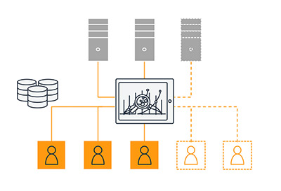
The following diagram illustrates a traditional architecture, which requires additional servers (and higher upfront cost) to scale.

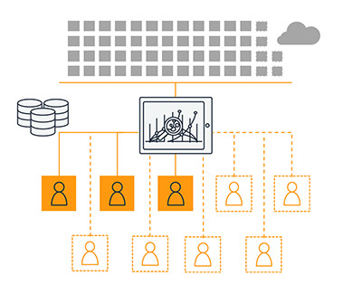
With QuickSight, you have access to the power and scale of the AWS Cloud. You get auto scaled, consistent performance no matter the concurrency or scale of the userbase, and a truly pay-per-use architecture, meaning you only pay when your users access the dashboards or reports. The following diagram illustrates how QuickSight scales seamlessly with its serverless architecture, powered by the AWS cloud.

Furthermore, QuickSight enables your users to perform machine learning based insights such as anomaly detection, forecasting, and natural language queries. It also has a rich set of APIs that allow you to programmatically manage your analytics workflows, such as moving dashboards across accounts, automating deployments, and managing access for users with single sign-on (SSO).

New features in QuickSight Embedded Analytics

We recently announced the launch of additional embedding capabilities that allow you to do even more with QuickSight embedded analytics. QuickSight now allows you to embed dashboard authoring within applications (such as SaaS applications and enterprise portals), allowing you to empower your end-users to create their own visualizations and reports.

These ad hoc data analysis and self-service data exploration capabilities mean you don’t have to repeatedly create custom dashboards based on requests from your end-users, and can provide end-users with even greater agility and transparency with their data. This capability helps create product differentiation and up-sell opportunities within customer applications.

With this launch, QuickSight also provides namespaces, a multi-tenant capability that allows you to easily maintain data isolation while supporting multiple workloads within the same QuickSight account. For example, if you’re an independent software vendor (ISV), you can now assign dedicated namespaces to different customers within the same QuickSight account. This allows you to securely manage multiple customer workloads as users (authors or readers) within one namespace, and they can only discover and share content with other users within the same namespace, without exposing any data to other parties.

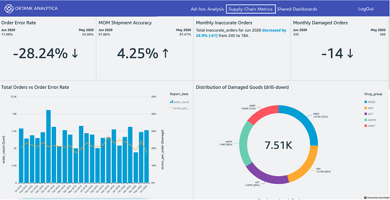
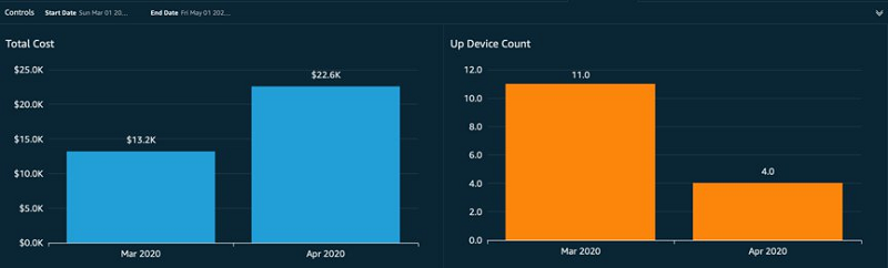
Without namespaces, you could set up your own embedded dashboards for hundreds of thousands of users with QuickSight. For example, see the following dashboard for our fictional company, Oktank Analytica.

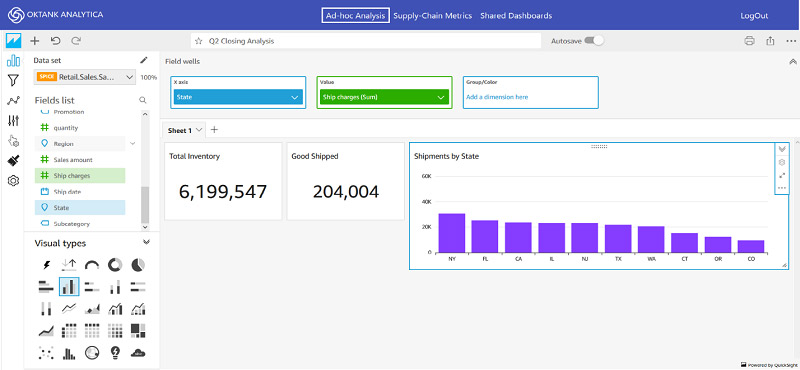
With namespaces in place, you can extend this to provide ad-hoc authoring capabilities using curated datasets specific to each customer, created and shared by the developer or ISV. See the following screenshot.

For more information about these new features, see Embed multi-tenant analytics in applications with Amazon QuickSight.

Customer success stories

Customers are already using embedded analytics in QuickSight to great success. In this section, we share the stories of a few customers.

Blackboard

Blackboard is a leading EdTech company, serving higher education, K-12, business, and government clients around the world.

“The recent wave in digital transformation in the global education community has made it clear that it’s time for a similar transformation in the education analytics tools that support that community,” says Rachel Scherer, Sr. Director of Data & Analytics at Blackboard. “We see a need to support learners, teachers, and leaders in education by helping to change their relationship with data and information—to reduce the distance between information and experience, between ‘informed’ and ‘acting.’

“A large part of this strategy involves embedding information directly where our users are collaborating, teaching, and learning—providing tools and insights that aid in assessment, draw attention to opportunities learners may be missing, and help strategic and academic leadership identify patterns and opportunities for intervention. We’re particularly interested in making the experience of being informed much more intuitive—favoring insight-informed workflows and/or embedded prose over traditional visualizations that require interpretation.

“By removing the step of interpretation, embedded visualizations make insights more useful and actionable. With QuickSight, we were able to deliver on our promise of embedding visualizations quickly, supporting the rapid iteration that we require, at the large scale needed to support our global user community.”

For more information about Blackboard’s QuickSight use case, see the AWS Online Tech Talk Embedding Analytics in your Applications with Amazon QuickSight at the 25:50 mark.

Comcast

Syndication Insights (SI) enables Comcast’s syndicated partners to access the same level of rich data insights that Comcast uses for platform and operational improvements.

“The SI platform enables partners to gain deeper business insights, such as early detection into anomalies for users, while ensuring a seamless experience through embedded, interactive reports,” says Ajay Gavagal, Sr. Manager of Software Development at Comcast. “From the start, scalability was a core requirement for us. We chose QuickSight as it is scalable, enabling SI to extend to multiple syndicated partners without having to provision or manage additional infrastructure. Furthermore, QuickSight provides interactive dashboards that can be easily embedded into an application. Lastly, QuickSight’s rich APIs abstract away a lot of functionality that would otherwise need to be custom built.”

For more information about how Comcast uses QuickSight, see the AWS Online Tech Talk Embedding Analytics in your Applications with Amazon QuickSight at the 38:05 mark.

Panasonic Avionics Corporation

Panasonic Avionics Corporation provides customized in-flight entertainment and communications systems to more than 300 airlines worldwide.

“Our cloud-based solutions collect large amounts of anonymized data that help us optimize the experience for both our airline partners and their passengers,” says Anand Desikan, Director of Cloud Operations at Panasonic Avionics Corporation. “We started using Amazon QuickSight to report on in-flight Wi-Fi performance, and with its rich APIs, pay-per-session pricing, and ability to scale, we quickly rolled out QuickSight dashboards to hundreds of users. The constant evolution of the platform has been impressive: ML-powered anomaly detection, Amazon SageMaker integration, embedding, theming, and cross-visual filtering. Our users consume insights via natural language narratives, which allows them to read all their information right off the dashboard with no complex interpretation needed.”

EHE Health

EHE Health is national preventive health and primary care Center of Excellence provider system.

“As a 106-year-old organization moving toward greater agility and marketplace nimbleness, we needed to drastically upgrade our ability to be transparent within our internal and external ecosystems,” says David Buza, Chief Technology Officer at EHE Health. “With QuickSight, we are not constrained by pre-built BI reports, and can easily customize and track the right operational metrics, such as product utilization, market penetration, and available inventory to gain a holistic view of our business. These inputs help us to understand current performance and future opportunity so that we can provide greater partnership to our clients, while delivering on our brand promise of creating healthier employee populations.

“QuickSight allowed our teams to seamlessly communicate with our clients—all viewing the same information, simultaneously. QuickSight’s embedding capabilities, along with its secure platform, intuitive design, and flexibility, allowed us to service all stakeholders—both internally and externally. This greater flexibility and customization allowed us to fit the client’s needs seamlessly.”

Conclusion

Where data agility and transparency are critical to business success, embedded analytics can open a universe of possibilities, and we are excited to see what our customers will do with these new capabilities.

Additional resources

For more resources, see the following:


About the Author

Dorothy Li is the Vice President and General Manager for Amazon QuickSight.

How Aruba Networks built a cost analysis solution using AWS Glue, Amazon Redshift, and Amazon QuickSight

Post Syndicated from Siddharth Thacker original https://aws.amazon.com/blogs/big-data/how-aruba-networks-built-a-cost-analysis-solution-using-aws-glue-amazon-redshift-and-amazon-quicksight/

This is a guest post co-written by Siddharth Thacker and Swatishree Sahu from Aruba Networks.

Aruba Networks is a Silicon Valley company based in Santa Clara that was founded in 2002 by Keerti Melkote and Pankaj Manglik. Aruba is the industry leader in wired, wireless, and network security solutions. Hewlett-Packard acquired Aruba in 2015, making it a wireless networking subsidiary with a wide range of next-generation network access solutions.

Aruba Networks provides cloud-based platform called Aruba Central for network management and AI Ops. Aruba cloud platform supports thousands of workloads to support customer facing production environment and also a separate development platform for Aruba engineering.

The motivation to build the solution presented in this post was to understand the unit economics of the AWS resources used by multiple product lines across different organization pillars. Aruba wanted a faster, effective, and reliable way to analyze cost and usage data and visualize that into a dashboard. This solution has helped Aruba in multiple ways, including:

  • Visibility into costs – Multiple Aruba teams can now analyze the cost of their application via data surfaced with this solution
  • Cost optimization – The solution helps teams identify new cost-optimization opportunities by making them aware of the higher-cost resources with low utilization so they can optimize accordingly
  • Cost management – The Cloud DevOps organization, the group who built this solution, can effectively plan at the application level and have a direct positive impact on gross margins
  • Cost savings – With daily cost data available, engineers can see the monetary impact of right-sizing compute and other AWS resources almost immediately
  • Big picture as well as granular – Users can visualize cost data from the top down and track cost at a business level and a specific resource level

Overview of the solution

This post describes how Aruba Networks automated the solution, from generating the AWS Cost & Usage Report (AWS CUR) to its final visualization on Amazon QuickSight. In this solution, they start by configuring the CUR on their primary payer account, which publishes the billing reports to an Amazon Simple Storage Service (Amazon S3) bucket. Then they use an AWS Glue crawler to define and catalog the CUR data. As the new CUR data is delivered daily, the data catalog is updated, and the data is loaded into an Amazon Redshift database using Amazon Redshift Spectrum and SQL. The reporting and visualization layer is built using QuickSight. Finally, the entire pipeline is automated by using AWS Data Pipeline.

The following diagram illustrates this architecture.

Aruba prefers the AWS CUR Report to AWS Cost Explorer because AWS Cost Explorer provides usage information at a high level, and not enough granularity for detailed operations, such as data transfer cost. AWS CUR provides the most detailed information available about your AWS costs and usage at an hourly granularity. This allows the Aruba team to drill down the costs by the hour or day, product or product resource, or custom tags, enabling them to achieve their goals.

Aruba implemented the solution with the following steps:

  1. Set up the CUR delivery to a primary S3 bucket from the billing dashboard.
  2. Use Amazon S3 replication to copy the primary payer S3 bucket to the analytics bucket. Having a separate analytics account helps prevent direct access to the primary account.
  3. Create and schedule the crawler to crawl the CUR data. This is required to make the metadata available in the Data Catalog and update it quickly when new data arrives.
  4. Create respective Amazon Redshift schema and tables.
  5. Orchestrate an ETL flow to load data to Amazon Redshift using Data Pipeline.
  6. Create and publish dashboards using QuickSight for executives and stakeholders.

Insights generated

The Aruba DevOps team built various reports that provide the cost classifications on AWS services, weekly cost by applications, cost by product, infrastructure, resource type, and much more using the detailed CUR data as shown by the following screenshot.

For example, using the following screenshot, Aruba can conveniently figure out that compute cost is the biggest contributor compared to other costs. To reduce the cost, they can consider using various cost-optimization methods like buying reserved instances, savings plans, or Spot Instances wherever applicable.

Similarly, the following screenshot highlights the cost doubled compared to the first week of April. This helps Aruba to identify anomalies quickly and make informed decisions.

Setting up the CUR delivery

For instructions on setting up a CUR, see Creating Cost and Usage Reports.

To reduce complexity in the workflow, Aruba chose to create resources in the same region with hourly granularity, mainly to see metrics more frequently.

To lower the storage costs for data files and maximize the effectiveness of querying data with serverless technologies like Amazon Athena, Amazon Redshift Spectrum, and Amazon S3 data lake, save the CUR in Parquet format. The following screenshot shows the configuration for delivery options.

The following table shows some example CUR data.

bill_payer_account_id line_item_usage_account_id line_item_usage_start_date line_item_usage_end_date line_item_product_code line_item_usage_type line_item_operation
123456789 111222333444 00:00.0 00:00.0 AmazonEC2 USW2-EBS:VolumeP-IOPS.piops CreateVolume-P-IOPS
123456789 111222333444 00:00.0 00:00.0 AmazonEC2 USW2-APN1-AWS-In-Bytes LoadBalancing-PublicIP-In
123456789 111222333444 00:00.0 00:00.0 AmazonEC2 USW2-DataProcessing-Bytes LoadBalancing
123456789 111222333444 00:00.0 00:00.0 AmazonEC2 USW2-EBS:SnapshotUsage CreateSnapshot
123456789 555666777888 00:00.0 00:00.0 AmazonEC2 USW2-EBS:SnapshotUsage CreateSnapshot
123456789 555666777888 00:00.0 00:00.0 AmazonEC2 USW2-DataTransfer-Regional-Bytes InterZone-In
123456789 555666777888 00:00.0 00:00.0 AmazonS3 USW2-Requests-Tier2 ReadLocation
123456789 555666777888 00:00.0 00:00.0 AmazonEC2 USW2-DataTransfer-Regional-Bytes InterZone-In

Replicating the CUR data to your analytics account

For security purposes, other teams aren’t allowed to access the primary (payer) account, and therefore can’t access CUR data generated from that account. Aruba replicated the data to their analytics account and build the cost analysis solution there. Other teams can access the cost data without getting access permission for the primary account. The data is replicated across accounts by adding an Amazon S3 replication rule in the bucket. For more information, see Adding a replication rule when the destination bucket is in a different AWS account.

Cataloging the data with a crawler and scheduling it to run daily

Because AWS delivers all daily reports in a report date range report-prefix/report-name/yyyymmdd-yyyymmdd folder, Aruba uses AWS Glue crawlers to crawl through the data and update the catalog.

AWS Glue is a fully managed ETL service that makes it easy to prepare and load the data for analytics. Once the AWS Glue is pointed to the data stored on AWS, it discovers the data and stores the associated metadata (such as table definition and schema) in the Data Catalog. After the data is cataloged, the data is immediately searchable, queryable, and available for ETL. For more information, see Populating the AWS Glue Data Catalog.

The following screenshot shows the crawler created on Amazon S3 location of the CUR data.

The following code is an example table definition populated by the crawler.:

CREATE EXTERNAL TABLE `cur_parquet`(
  `identity_line_item_id` string, 
  `identity_time_interval` string, 
  `bill_invoice_id` string, 
………
………
  `resource_tags_user_infra_role` string)

PARTITIONED BY ( 
  `year` string, 
  `month` string )

ROW FORMAT SERDE  'org.apache.hadoop.hive.ql.io.parquet.serde.ParquetHiveSerDe'
STORED AS INPUTFORMAT   'org.apache.hadoop.hive.ql.io.parquet.MapredParquetInputFormat' 
OUTPUTFORMAT   'org.apache.hadoop.hive.ql.io.parquet.MapredParquetOutputFormat'
LOCATION
  's3://curS3bucket/Parquet/'

Transforming and loading using Amazon Redshift

Next in the analytics service, Aruba chose Amazon Redshift over Athena. Aruba has a use case to integrate cost data together with other tables already present in Amazon Redshift and hence using the same service makes it easy to integrate with their existing data. To further filter and transform data at the same time, and simplify the multi-step ETL, Aruba chose Amazon Redshift Spectrum. It helps to efficiently query and load CUR data from Amazon S3. For more information, see Getting started with Amazon Redshift Spectrum.

Use the following query to create an external schema and map it to the AWS Glue database created earlier in the Data Catalog:

--Choose a schema name of your choice, cur_redshift_external_schema name is just an example--
 create external schema cur_redshift_spectrum_external_schema from data catalog database 
 'aruba_curr_db' iam_role 'arn:aws:iam::xxxxxxxxxxxxx:role/redshiftclusterrole' 
 create external database if not exists;

The table created in the Data Catalog appears under the Amazon Redshift Spectrum schema. The schema, table, and records created can be verified with the following SQL code:

SELECT Count(*) 
FROM   cur_redshift_spectrum_external_schema.<TABLE>; 

--Query the right partition, year=2020 and month=2 is used an example
SELECT Count(*) 
FROM   cur_redshift_spectrum_external_schema.<TABLE> 
WHERE  year=2020 
AND    month=2;

Next, transform and load the data into the Amazon Redshift table. Aruba started by creating an Amazon Redshift table to contain the data. The following SQL code can be used to create the production table with the desired columns:

CREATE TABLE redshift_schema.redshift_table 
  ( 
     usage_start_date TIMESTAMP, 
     usage_end_date   TIMESTAMP, 
     service_region   VARCHAR (256), 
     service_az       VARCHAR (256), 
     aws_resource_id  VARCHAR (256), 
     usage_amount     FLOAT (17), 
     charge_currency  VARCHAR (256), 
     aws_product_name VARCHAR (256), 
     instance_family  VARCHAR (256), 
     instance_type    VARCHAR (256), 
     unblended_cost   FLOAT (17), 
     usage_cost       FLOAT (17)
  ); 

CUR is dynamic in nature, which means that some columns may appear or disappear with each update. When creating the table, we take static columns only. For more information, see Line item details.

Next, insert and update to ingest the data from Amazon S3 to the Amazon Redshift table. Each CUR update is cumulative, which means that each version of the CUR includes all the line items and information from the previous version.

The reports generated throughout the month are estimated and subject to change during the rest of the month. AWS finalizes the report at the end of each month. Finalized reports have the calculations for the blended and unblended costs, and cover all the usage for the month. For this use case, Aruba updates the last 45 days of data to make sure the finalized cost is captured. The below sample query can be used to verify the updated data:

-- Create Table Statement
 INSERT INTO redshift_schema.redshift_table
            (usage_start_date, 
             usage_end_date, 
             service_region, 
             service_az, 
             aws_resource_id, 
             usage_amount, 
             charge_currency, 
             aws_product_name, 
             instance_family, 
             instance_type, 
             unblended_cost,
             Usage_Cost ) 
 SELECT line_item_usage_start_date, 
       line_item_usage_end_date, 
       line_item_operation, 
       line_item_availability_zone, 
       line_item_resource_id, 
       line_item_usage_amount, 
       line_item_currency_code, 
       product_product_name, 
       product_instance_family, 
       product_instance_type, 
       line_item_unblended_cost,
       case when line_item_type='Usage' then line_item_unblended_cost
            else 0
            end as usage_cost 
 FROM   cur_redshift_external_schema.cur_parquet_parquet
 WHERE  line_item_usage_start_date >= date_add('day', -45, getdate()) 
       AND line_item_usage_start_date < date_add('day', 1, getdate()); 

Using Data Pipeline to orchestrate the ETL workflow

To automate this ETL workflow, Aruba chose Data Pipeline. Data Pipeline helps to reliably process and move data between different AWS compute and storage services, as well as on-premises data sources. With Data Pipeline, Aruba can regularly access their data where it’s stored, transform and process it at scale, and efficiently transfer the results to AWS services such as Amazon S3, Amazon Relational Database Service (Amazon RDS), Amazon DynamoDB, and Amazon EMR. Although the detailed steps of setting up this pipeline are out of scope for this blog, there is a sample workflow definition JSON file, which can be imported after making the necessary changes.

Data Pipeline workflow

The following screenshot shows the multi-step ETL workflow using Data Pipeline. Data Pipeline is used to run the INSERT query daily, which inserts and updates the latest CUR data into our Amazon Redshift table from the external table.

In order to copy data to Amazon Redshift,  RedshiftDataNode and RedshiftCopyActivity can be used, and then scheduled to run periodically.

Sharing metrics and creating visuals with QuickSight

To share the cost and usage with other teams, Aruba choose QuickSight using Amazon Redshift as the data source. QuickSight is a native AWS service that seamlessly integrates with other AWS services such as Amazon Redshift, Athena, Amazon S3, and many other data sources.

As a fully managed service, QuickSight lets Aruba to easily create and publish interactive dashboards that include ML Insights. In addition to building powerful visualizations, QuickSight provides data preparation tools that makes it easy to filter and transform the data into the exact needed dataset. As a cloud-native service, dashboards can be accessed from any device and embedded into applications and portals, allowing other teams to monitor their resource usage easily. For more information about creating a dataset, see Creating a Dataset from a Database. Quicksight Visuals can then be created from this dataset.

The following screenshot shows a visual comparison of device cost and count to help find the cost per device. This visual helped Aruba quickly identify the cost per device increase in April and take necessary actions.

Similarly, the following visualization helped Aruba identify an increase in data transfer cost and helped them decide to invest in rearchitecting their application.

The following visualization classifies the cost spend per resource.

Conclusion

In this post, we discussed how Aruba Networks was able to successfully achieve the following:

  • Generate CUR and use AWS Glue to define data, catalog the data, and update the metadata
  • Use Amazon Redshift Spectrum to transform and load the data to Amazon Redshift tables
  • Query, visualize, and share the data stored using QuickSight
  • Automate and orchestrate the entire solution using Data Pipeline

Aruba use this solution to automatically generate a daily cost report and share it with their stakeholders, including executives and cloud operations team.


About the Authors

Siddharth Thacker works in Business & Finance Strategy in Cloud Software division at Aruba Networks. Siddharth has Master’s in Finance with experience in industries like banking, investment management, cloud software and focuses on business analytics, margin improvement and strategic partnerships at Aruba. In his spare time, he likes exploring outdoors and participate in team sports.

Swatishree Sahu is a Technical Data Analyst at Aruba Networks. She has lived and worked in India for 7 years as an SME for SOA-based integration tools before coming to US to pursue her master’s in Business Analytics from UT Dallas. Breaking down and analyzing data is her passion. She is a Star Wars geek, and in her free time, she loves gardening, painting, and traveling.

Ritesh Chaman is a Technical Account Manager at Amazon Web Services. With 10 years of experience in the IT industry, Ritesh has a strong background in Data Analytics, Data Management, and Big Data systems. In his spare time, he loves cooking (spicy Indian food), watching sci-fi movies, and playing sports.


Kunal Ghosh is a Solutions Architect at AWS. His passion is to build efficient and effective solutions on the cloud, especially involving Analytics, AI, Data Science, and Machine Learning. Besides family time, he likes reading and watching movies, and is a foodie.

Automate dataset monitoring in Amazon QuickSight

Post Syndicated from Ginni Malik original https://aws.amazon.com/blogs/big-data/automate-dataset-monitoring-in-amazon-quicksight/

Amazon QuickSight is an analytics service that you can use to create datasets, perform one-time analyses, and build visualizations and dashboards. In an enterprise deployment of QuickSight, you can have multiple dashboards, and each dashboard can have multiple visualizations based on multiple datasets. This can quickly become a management overhead to view all the datasets’ status with their latest refresh timestamp.

This post demonstrates how to visualize datasets associated with all the dashboards in your account, with their latest refresh status and refresh time.

Solution overview

The following screenshot illustrates the architecture of the solution.

The architecture includes the following steps:

  1. You create the datasets and tag them via an AWS Lambda
  2. A second function gets the refresh status from the tagged datasets.
  3. The function stores the refresh status in Amazon Simple Storage Service (Amazon S3).
  4. You query the refresh status in Amazon Athena.
  5. You visualize the refresh status in QuickSight.

A QuickSight deployment can have multiple dashboards and each dashboard can have multiple datasets associated with it. You can end up having hundreds of datasets. It’s difficult to know if all the underlying datasets are refreshing as required unless you check them manually. However, QuickSight sends email notifications to the dataset owner on its dataset refresh failure. This solution provides a holistic view of all datasets’ refreshes.

The aim is to create a dashboard that monitors the refresh of the existing datasets and provides refresh status for the datasets.

To implement the solution, you must create the following:

  • A Lambda execution role for QuickSight.
  • A scheduled Lambda function to tag the datasets.
  • A scheduled Lambda function to get the last refresh status of the datasets and store it in Amazon S3.
  • An external table in Athena on top of the S3 bucket.
  • A QuickSight dashboard using Athena as the data source, which provides the datasets’ last refresh status.

This post assumes that you have existing analyses and dashboards with numerous datasets.

Creating a Lambda execution role for QuickSight

Your first step is to create a Lambda execution role that allows you to perform tagging and create QuickSight analysis, datasets, and data sources. The role should be able to describe and update them. The following code is an example role policy (replace the bucket name with the bucket for storing the QuickSight ingestion results):

{
    "Version": "2012-10-17",
    "Statement": [
        {
            "Sid": "VisualEditor0",
            "Effect": "Allow",
            "Action": [
                "quicksight:CreateDashboard",
                "quicksight:List*",
                "quicksight:Describe*",
                "quicksight:Tag*",
                "tag:GetResources"
            ],
            "Resource": "*"
        },
        {
            "Sid": "VisualEditor1",
            "Effect": "Allow",
            "Action": "s3:PutObject",
            "Resource": [
                "arn:aws:s3:::bucket-name-to-store-ingestion/*"
            ]
        }
    ]
}

Creating a scheduled Lambda function to tag the datasets

The next step is to identify all the datasets required for your dashboard and tag them. It’s easier to do this right after you create the dataset. Complete the following steps:

  1. On the QuickSight console, choose Manage data.

  1. Choose your dataset and choose Edit dataset.

  1. Record the dataset ID from the URL (data-sets/<dataset ID>/prepare).

Alternatively, you can use a Lambda function to find the dataset name and ID. See the following code (replace the AwsAccountID with your ID):

import boto3
client = boto3.client('quicksight')
def lambda_handler(event, context):
    response=client.list_data_sets(
        AwsAccountId='1234567890',
        MaxResults=100
    )
    for r in response['DataSetSummaries']:
        dataset_info={}
        dataset_info['id']=r['DataSetId']
        dataset_info['name']=r['Name']
        print (dataset_info['name']+':'+dataset_info['id'])

The function provides all the datasets in your account. Make sure to record the dataset IDs specific to your dashboard.

  1. Create your Lambda function.
  2. Tag the datasets per your individual dashboards. See the following code (use the target dashboard name and ID to create the tagging key, and replace the dataset_ids and account number with your own):
import boto3
client = boto3.client('quicksight')
acct_id = '123456678788'
def lambda_handler(event, context):
    dataset_ids=['0e994f54-8d08-4b64-98ca-195cf7b46077','16d5bf20-4415-42d1-b54c-9aba95b13d67','5c5fd93a-0bb6-468f-a0c4-ff1c15597d20']
    for i in dataset_ids:
        response = client.tag_resource(
            ResourceArn='arn:aws:quicksight:us-east-1:123456678788:dataset/{}'.format(i),
            Tags=[
                {
                    'Key' : 'DashboardName',
                    'Value' : 'QuickSight_refresh_status_demo'
                }
                ]
                )

You can do this for all your dashboards. The only limitation is you can only tag one dataset to one dashboard name key pair.

If you tag the datasets with a wrong key, you can remove them using an untag call and replace the ResourceArn with the specific dataset ARN. See the following code:

     response = client.untag_resource(
    ResourceArn='arn:aws:quicksight:us-east-1:123456678788:dataset/794e28ae-2b89-49ef-b885-196c95bfd4f8',
    TagKeys=[
        'DashboardName'
    ]
    )

Creating a Lambda function to get the last refresh status

The next step is to configure a Lambda function that gets the last refresh status of the tagged datasets and loads it into Amazon S3. You use resourcegroupstaggingapi to get back all the resources with a particular key. For this post, the key is the DashboardName. From the response of the ResourceTagMappingList, you filter out the dataset ID and dataset ARN. You also get the data source ARN and name for each dataset associated with the particular key value. Finally, you list the ingestions for all the datasets and classify them as one of the following:

  • Failed – The last refresh failed.
  • Did not run within last 24 hours – No ingestion ID in the last 24 hours (the time is configurable). You explicitly use this status even if the previous run before the last 24 hours succeeded or failed. This makes sure the datasets adhere to a certain refresh schedule. For this post, you want the datasets to refresh one time a day.
  • Error – No ingestion ID for more than 90 days.

See the following code (replace the placeholder text with your specific values):

import json
import boto3
import csv
from botocore.exceptions import ClientError
from datetime import datetime
from datetime import timedelta
from datetime import timezone
import jmespath

glue = boto3.client('glue')
s3= boto3.client('s3')
client = boto3.client('resourcegroupstaggingapi')
client1 = boto3.client('quicksight')
dataset_ids=[]
AwsAccountId='123456678788'
def lambda_handler(event, context):
    items=[]
    tagfilters=[
        {
            'Key': 'DashboardName',
            'Values': [
                'QuickSight_refresh_status_demo'
                            #add dashboard name
            ]
        },
    ]


    response = client.get_resources(
    TagFilters=tagfilters
    )
    
    # Get the response back for each of the above listed Key Values
    resources = response['ResourceTagMappingList']
    for resource in resources:
        perm=""
        data={}
        permission=[]
        data['resource_ARN']=resource['ResourceARN']
        dataset_id_arn=data['resource_ARN'].split('/')
        data['dataset_id']=dataset_id_arn[1]
        # For each of the above dataset , describe the dataset to get the data source
        response = client1.describe_data_set(
                 AwsAccountId=AwsAccountId,
                 DataSetId=data['dataset_id']
        )

        datasourcearn = jmespath.search('DataSet.PhysicalTableMap.*.*.DataSourceArn',response)
        datasourcearnid= str(datasourcearn[0]).split('/')
        datasourcearnid=datasourcearnid[1]
        datasourcearnid=datasourcearnid.replace("']",'')
        data['DatasetName']=response.get('DataSet').get('Name')
        response = client1.describe_data_source(
            AwsAccountId=AwsAccountId,
            DataSourceId=datasourcearnid
        )
        datasourcename=response.get('DataSource').get('Name')
        data['DataSourceName']=datasourcename
        resource_tags = resource['Tags']
        for tag in resource_tags:

                if tag['Key'] == 'DashboardName':
                    data['dashboard_name'] = tag['Value']

        response1= client1.list_ingestions(
            DataSetId=data['dataset_id'],
            AwsAccountId=AwsAccountId,
            MaxResults=1  # To get the latest ingestion, if you want history you can change this number
        )

        if response1.get('Ingestions'):
            for i in response1['Ingestions']:
                data['IngestionId']=i['IngestionId']
                data['CreatedTime']=i['CreatedTime']
                try:
                    response = client1.describe_ingestion(DataSetId=data['dataset_id'],IngestionId=data['IngestionId'],AwsAccountId=AwsAccountId)

                    if  response:
                        data['Time']=str(response['Ingestion']['CreatedTime'])
                        if ((datetime.utcnow() - response['Ingestion']['CreatedTime'].replace(tzinfo=None)).total_seconds()) >= (24*60*60):  #Check the refresh status within last 24 hours, you can change this per your requirement
                            data['Status']='Did not run within last 24 hrs'
                        else:
                            data['Status']=response['Ingestion']['IngestionStatus']
                except ClientError as e:
                    data['Time']='Failed, Check if dataset is being used'
                    data['Status']=e.response['Error']['Message']

            items.append(data)


    row=['DashboardName,DatsetName,Status,Time,DataSourceName']
    csv_key='quicksight-dashboard-metada/report.csv'


    for data in items:

        row.append(data['dashboard_name'] +','+data['DatasetName']+','+data['Status']+','+data['Time']+','+data['DataSourceName'])
    values = '\n'.join(str(v) for v in row)

    response = s3.put_object(
        Body=values,
        Bucket='bucketname',
        Key=csv_key
    )

The last status run is now stored in a .csv file in the specific bucket mentioned in the Lambda function (see the following screenshot).

You can also schedule your function to run at a certain frequency, depending on when you want to check the status.

Creating an external table in Athena on top of Amazon S3

Now you can create an external Athena table on top of the .csv file you stored in Amazon S3 and query it. Use the following table definition for reference (replace the location with the location of your S3 bucket):

CREATE EXTERNAL TABLE IF NOT EXISTS qs_meta_table
( `DashboardName` string, 
 `DatasetName` string, 
 `Status` string, 
 `LastRefershTime` string, 
 `DataSourceName` string ) 
 ROW FORMAT SERDE 'org.apache.hadoop.hive.serde2.OpenCSVSerde' WITH SERDEPROPERTIES 
 ( "separatorChar" = "," )
 LOCATION 's3://bucketname/quicksight-dashboard-metada/' 
 TBLPROPERTIES ( "skip.header.line.count"="1")

You can get the latest status of the dataset refreshes by querying the table with SQL in Athena.

Creating a QuickSight dashboard using Athena as the data source

To visualize this data and share it with others, build a dashboard on top of the data in QuickSight. The following screenshot shows the listed dashboards.

You first create a dataset for the Athena table.

  1. On the QuickSight console, choose Manage data.
  2. Choose Create dataset.

You use Athena as the source for your dataset. If you don’t have an existing Athena data source, you can create a new one. For instructions, see Creating a Data Source.

  1. Choose the table you just created.

  1. Select Import to SPICE for quicker analysis.

Depending on the size of your dataset and expected latency, you can choose Directly query your data instead. If you use SPICE, remember to add a refresh schedule for the dataset.

  1. Create an analysis from the dataset.

For this post, choose a table visual type and drag all the columns to the Value field well.

You can create the visualization as in the following screenshot, with conditional formatting to highlight failed and successful loads.

  1. To publish the dashboard, choose Share on the application bar of the analysis.
  2. Choose Publish dashboard.

  1. For Publish new dashboard as, enter a name for your dashboard.

You can now share the dashboard with end-users.

Conclusion

In this post, we described how to create a QuickSight dashboard that can track the last refresh status of all the datasets in your account. The dashboard provides a single pane view of the status of all the datasets and avoids the manual effort of opening and checking each individual dataset.


About the authors

Ginni Malik is an Associate Cloud Developer with AWS.


Rohan Jamadagni is a Solutions Architect with AWS.