Post Syndicated from Ankush Goyal original https://aws.amazon.com/blogs/security/how-to-use-aws-verified-access-logs-to-write-and-troubleshoot-access-policies/
On June 19, 2023, AWS Verified Access introduced improved logging functionality; Verified Access now logs more extensive user context information received from the trust providers. This improved logging feature simplifies administration and troubleshooting of application access policies while adhering to zero-trust principles.
In this blog post, we will show you how to manage the Verified Access logging configuration and how to use Verified Access logs to write and troubleshoot access policies faster. We provide an example showing the user context information that was logged before and after the improved logging functionality and how you can use that information to transform a high-level policy into a fine-grained policy.
Overview of AWS Verified Access
AWS Verified Access helps enterprises to provide secure access to their corporate applications without using a virtual private network (VPN). Using Verified Access, you can configure fine-grained access policies to help limit application access only to users who meet the specified security requirements (for example, user identity and device security status). These policies are written in Cedar, a new policy language developed and open-sourced by AWS.
Verified Access validates each request based on access policies that you set. You can use user context—such as user, group, and device risk score—from your existing third-party identity and device security services to define access policies. In addition, Verified Access provides you an option to log every access attempt to help you respond quickly to security incidents and audit requests. These logs also contain user context sent from your identity and device security services and can help you to match the expected outcomes with the actual outcomes of your policies. To capture these logs, you need to enable logging from the Verified Access console.
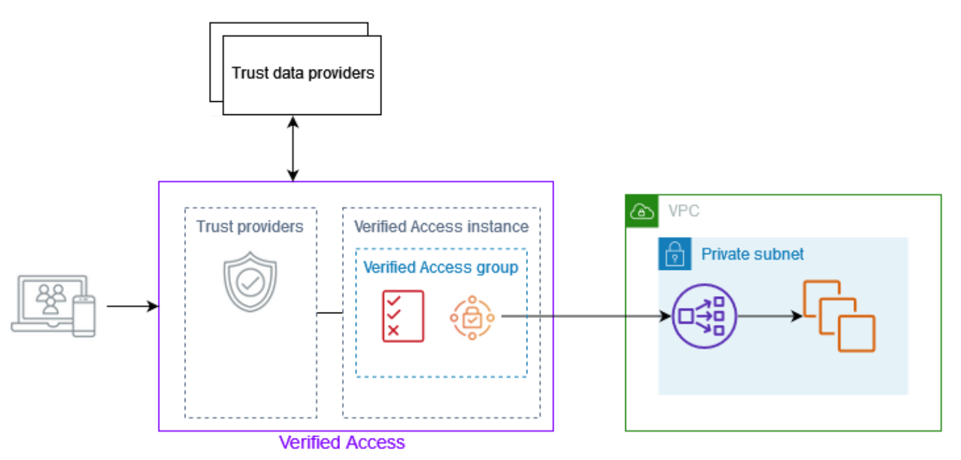
Figure 1: Overview of AWS Verified Access architecture showing Verified Access connected to an application
After a Verified Access administrator attaches a trust provider to a Verified Access instance, they can write policies using the user context information from the trust provider. This user context information is custom to an organization, and you need to gather it from different sources when writing or troubleshooting policies that require more extensive user context.
Now, with the improved logging functionality, the Verified Access logs record more extensive user context information from the trust providers. This eliminates the need to gather information from different sources. With the detailed context available in the logs, you have more information to help validate and troubleshoot your policies.
Let’s walk through an example of how this detailed context can help you improve your Verified Access policies. For this example, we set up a Verified Access instance using AWS IAM Identity Center (successor to AWS Single Sign-on) and CrowdStrike as trust providers. To learn more about how to set up a Verified Access instance, see Getting started with Verified Access. To learn how to integrate Verified Access with CrowdStrike, see Integrating AWS Verified Access with device trust providers.
Then we wrote the following simple policy, where users are allowed only if their email matches the corporate domain.
Before improved logging, Verified Access logged basic information only, as shown in the following example log.
Modify an existing Verified Access instance
To improve the preceding policy and make it more granular, you can include checks for various user and device details. For example, you can check if the user belongs to a particular group, has a verified email, should be logging in from a device with an OS that has an assessment score greater than 50, and has an overall device score greater than 15.
Modify the Verified Access instance logging configuration
You can modify the instance logging configuration of an existing Verified Access instance by using either the AWS Management Console or AWS Command Line Interface (AWS CLI).
- Open the Verified Access console and select Verified Access instances.
- Select the instance that you want to modify, and then, on the Verified Access instance logging configuration tab, select Modify Verified Access instance logging configuration.

Figure 2: Modify Verified Access logging configuration
- Under Update log version, select ocsf-1.0.0-rc.2, turn on Include trust context, and select where the logs should be delivered.
Figure 3: Verified Access log version and trust context


After you’ve completed the preceding steps, Verified Access will start logging more extensive user context information from the trust providers for every request that Verified Access receives. This context information can have sensitive information. To learn more about how to protect this sensitive information, see Protect Sensitive Data with Amazon CloudWatch Logs.
The following example log shows information received from the IAM Identity Center identity provider (IdP) and the device provider CrowdStrike.
The following example log shows the user context information received from the OpenID Connect (OIDC) trust provider Okta. You can see the difference in the information provided by the two different trust providers: IAM Identity Center and Okta.
The following is a sample policy written using the information received from the trust providers.
This policy only grants access to users who belong to a particular group, have a verified email address, and have a corporate email domain. Also, users can only access the application from a device with an OS that has an assessment score greater than 50, and has an overall device score greater than 15.
Conclusion
In this post, you learned how to manage Verified Access logging configuration from the Verified Access console and how to use improved logging information to write AWS Verified Access policies. To get started with Verified Access, see the Amazon VPC console.
If you have feedback about this post, submit comments in the Comments section below. If you have questions about this post, contact AWS Support.
Want more AWS Security news? Follow us on Twitter.