Post Syndicated from Grab Tech original https://engineering.grab.com/pinot-partnergateway-tech-blog

Introduction

Grab operates as a dynamic ecosystem involving partners and various service providers, necessitating real-time intelligence and decision-making for seamless integration and service delivery. To facilitate this, GrabDeveloper serves as Grab’s centralized platform for developers and partners. It supports API integration, partner onboarding, and product management. It also provides tech support through staging and production portals with detailed documentation.

Working alongside Developer Home, Partner Gateway acts as Grab’s secure interface for exposing APIs to third-party entities. It enables seamless interactions between Grab’s hosted services and external consumers, such as mobile apps, web browsers, and partners. Partner Gateway enhances the experience by offering advanced metrics tracking through time-series charts and dashboards. Partner Gateway delivers actionable insights that ensure high performance, reliability, and user satisfaction in application integrations with Grab services.

Use cases

Let’s explore GrabDeveloper integration use cases with one of our partners, whom we’ll refer to as “Alpha.” Alpha is a company that specializes in producing and distributing a diverse range of perishable goods. To optimize their operations, time-series charts tracking API traffic request status codes and average API response times play a crucial role.

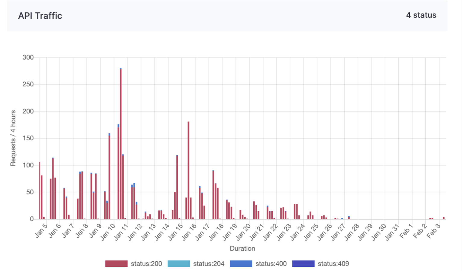
API traffic request service status codes chart

Time-series charts tracking API traffic request status codes offer valuable insights into the performance and reliability of APIs used for managing supply chain logistics, customer orders, and distribution networks. By monitoring these status codes, Alpha can promptly detect and resolve disruptions or failures in their digital systems, ensuring seamless operations and minimizing downtime.

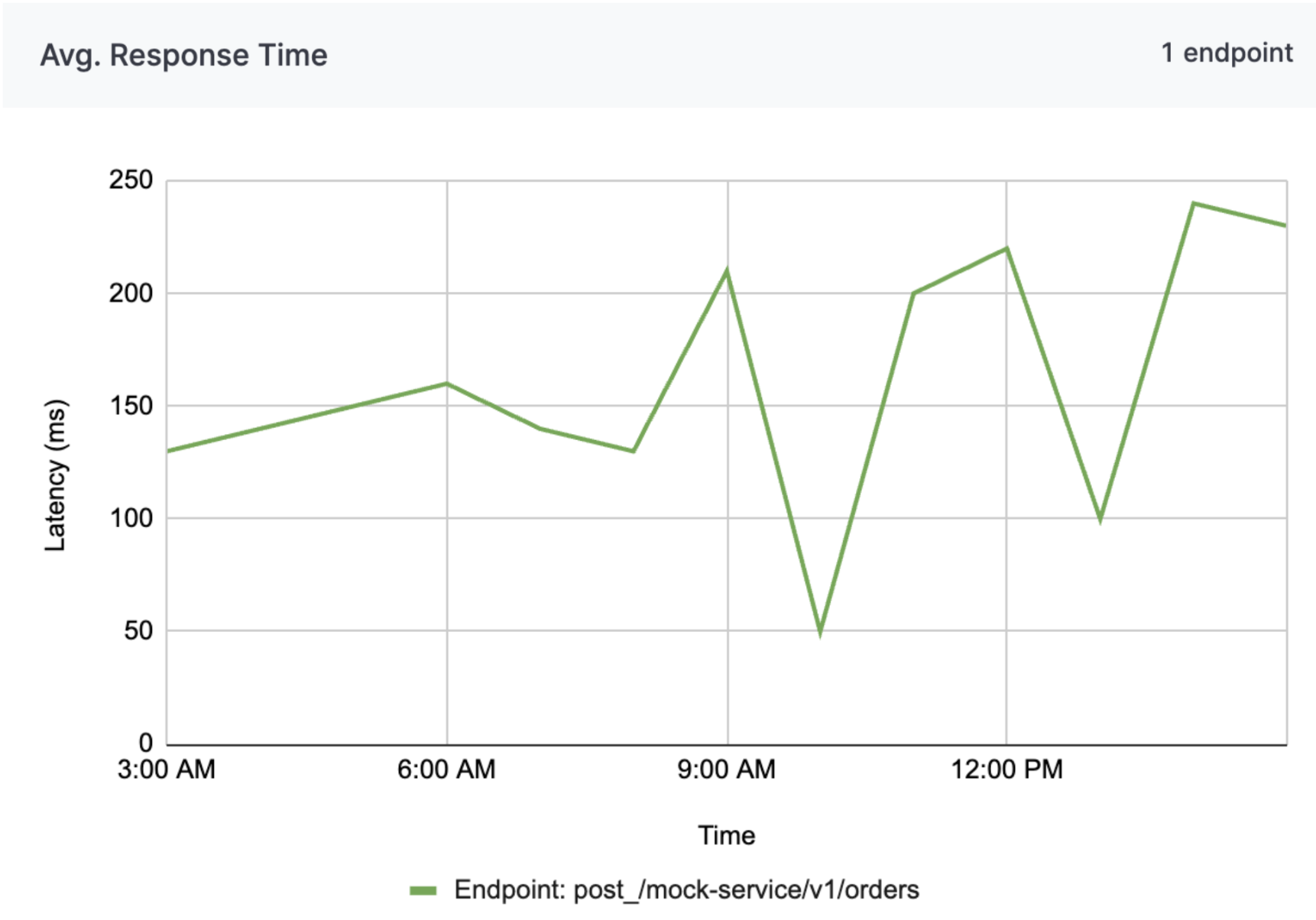
API average response times chart

Analyzing average response times helps the company maintain efficient communication between various systems, enhancing the speed and reliability of transactions and data exchanges. This proactive monitoring supports Alpha in delivering consistent, high-quality service to customers and partners, ultimately contributing to improved operational efficiency and customer satisfaction.

Analyzing average response times enables a company to ensure efficient communication across various systems, enhancing transaction speed and data exchange reliability. Proactive monitoring helps Alpha deliver consistent, high-quality service to customers and partners, boosting operational efficiency and customer satisfaction.

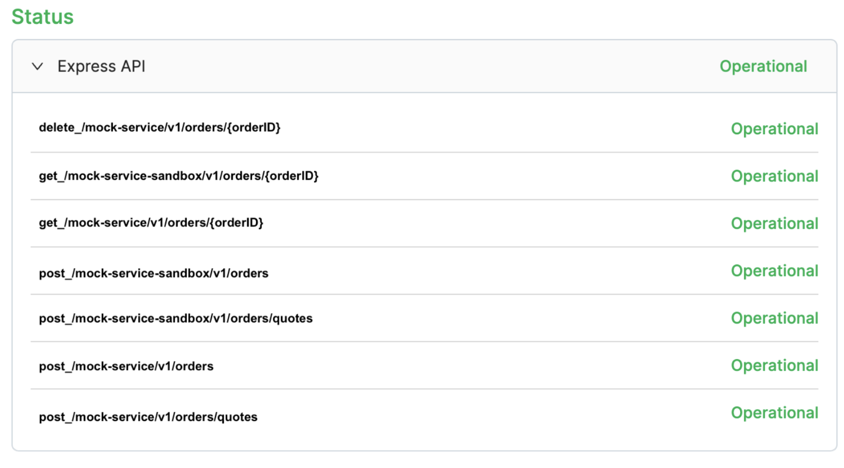
Endpoint status dashboard

For Alpha, the endpoint status dashboard delivers real-time insights into API performance, enabling swift issue resolution and seamless integration with the company’s systems. The dashboard enhances service reliability, supports business operations, and ensures uninterrupted data exchange, all of which are critical for Alpha’s business processes and customer satisfaction. Furthermore, the transparency and reliability provided by the dashboard strengthens trust in the partnership, ensuring Alpha to confidently rely on the integration to drive their digital initiatives and operational goals.

Why choose Apache Pinot and what is it?

To accommodate these use cases, we need a backend storage system engineered for low-latency queries across a wide range of temporal intervals, spanning from one-hour snapshots to 30-day retrospective analyses, whereby it could contain up to ~6.8 billion rows of data in a 30 day period for a particular dataset. This led us to choose Apache Pinot for these use cases, a distributed Online Analytical Processing (OLAP) system designed for low-latency analytical queries on large-scale data with millisecond query latencies.

Apache Pinot is a real-time distributed OLAP datastore designed to deliver low-latency analytics on large-scale data. It is optimized for high-throughput ingestion and real-time query processing making it ideal for scenarios such as user-facing analytics, dashboards, and anomaly detection. Apache Pinot supports complex queries, including aggregations and filtering. It delivers sub-second response times by leveraging techniques like columnar storage, indexing, and data partitioning to achieve efficient query execution.

Data ingestion process

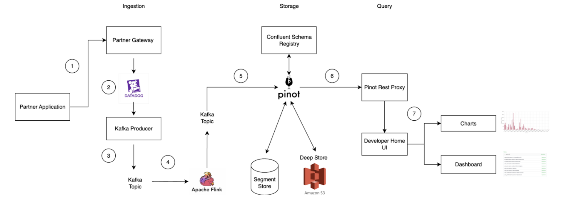
1. API call initiation: An API call is made on the partner application and routed through the Partner Gateway.
2. Metric tracking: Dimensions such as client ID, partner ID, status code, endpoint, metric name, timestamp, and value (which is the metric) are tracked and uploaded to Datadog, a cloud-based monitoring platform.
3. Kafka message transformation: Within the partner gateway code, an Apache Kafka Producer converts these metrics into Kafka messages and stores them in a Kafka Topic. Grab utilizes Protobuf for serialization and deserialization of Kafka messages. Since Grab’s Golang Kafka ecosystem does not use the Confluent Schema Registry, Kafka messages must be serialized with a magic byte which indicates that they are using Confluent’s Schema Registry, followed by the Schema ID.
4. Serialization via Apache Flink: Serialization is managed using Apache Flink, an open-source stream processing framework. This ensures compatibility with the Confluent Schema Registry Protobuf Decoder plugin on Apache Pinot. The messages are then written to a separate Kafka Topic.
5. Ingestion to Apache Pinot: Messages from the Kafka Topic containing the magic byte are ingested directly into Pinot, which references the Confluent Schema Registry to accurately deserialize the messages.
6. Query execution: Queries on the Pinot table can be executed via the Pinot Rest Proxy API.
7. Data visualization: Users can view their project charts and dashboards on the GrabDeveloper Home UI, where data points are retrieved from queries executed in step 6.

Challenges faced

During the initial setup, we encountered significant performance challenges when executing aggregation queries on large datasets exceeding 150GB. Specifically, attempts to retrieve and process data for periods ranging from 20 to 30 days resulted in frequent timeout issues as the queries took longer than 10 seconds. This was particularly concerning as it compromised our ability to meet our Service Level Agreement (SLA) of delivering query results within 300 milliseconds. The existing query infrastructure struggled to efficiently manage the volume and complexity of data within the required timeframe, necessitating optimization efforts to improve performance and reliability.

Solution

Drawing from the insights gained on the limitations of our initial solutions, we implemented these strategic optimizations to significantly enhance our table’s performance.

Partitioning by metric name

• Improved data locality: Partitioning the Kafka Topic by metric name ensures that related data is grouped together. When a query filters on a specific metric, Pinot can directly access the relevant partitions, minimizing the need to scan unrelated data. This significantly reduces I/O overhead and processing time.
• Efficient query pruning: By physically partitioning data, only the servers holding the relevant partitions are queried. This leads to more efficient query pruning, as irrelevant data is excluded early in the process, further optimizing performance.
• Enhanced parallel processing: Partitioning enables Pinot to distribute queries across multiple nodes, allowing different metrics to be processed in parallel. This leverages distributed computing resources, accelerating query execution and improving scalability for large datasets.

Column based on aggregation intervals

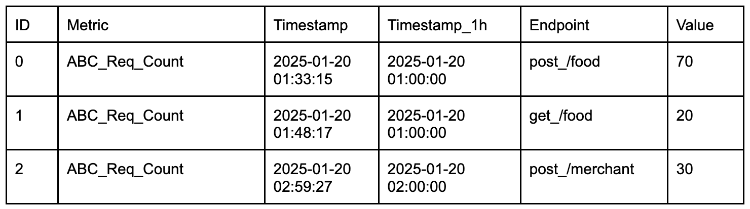
• Facilitates time-based aggregations: Rounded time columns (e.g., Timestamp_1h for hourly intervals) group data into coarser time buckets, enabling efficient aggregations such as hourly or daily metrics. This simplifies indexing and optimizes storage by precomputing aggregates for specific time intervals.
• Efficient data filtering: Rounded time columns allow for precise filtering of data within specific aggregation intervals. For example, the query SELECT SUM(Value) FROM Table WHERE Timestamp_1h = '2025-01-20 01:00:00' can exclude irrelevant columns (e.g., column 2) and focus only on rows within the specified time interval, further enhancing query efficiency.

Utilizing the Star-tree index in Apache Pinot

The Star-tree Index in Apache Pinot is an advanced indexing structure that enhances query performance by pre-aggregating data across multiple dimensions (e.g., D1, D2). It features a hierarchical tree with a root node, leaf nodes (holding up to T records), and non-leaf nodes that split into child nodes when exceeding T records. Special star nodes store pre-aggregated records by omitting the splitting dimension. The tree is constructed based on a dimensionSplitOrder, dictating node splitting at each level.

Sample table configuration for Star-tree index:

"tableIndexConfig": {
  "starTreeIndexConfigs": [{
    "dimensionsSplitOrder": [
      "Metric",
      "Endpoint",
      "Timestamp_1h"
    ],
    "skipStarNodeCreationForDimensions": [
    ],
    "functionColumnPairs": [
      "AVG__Value"
    ],
    "maxLeafRecords": 1
  }],
  ...
}

Configuration explanation:

• dimensionsSplitOrder: This specifies the order in which dimensions are split at each level of the tree. The order is “Metric”, “Endpoint”, “Timestamp_1h”. This means the tree will first split by Metric, then by Endpoint, and finally by Timestamp_1h.
• skipStarNodeCreationForDimensions: This array is empty, indicating that star nodes will be created for all dimensions specified in the split order. No dimensions are omitted from star node creation.
• functionColumnPairs: This specifies the aggregation functions to be applied to columns when creating star nodes. The configuration includes “AVG__Value”, meaning the average of the “Value” column will be calculated and stored in star nodes.
• maxLeafRecords: This is set to 1, indicating that each leaf node will contain only one record. If a node exceeds this number, it will split into child nodes.

Star-tree diagram

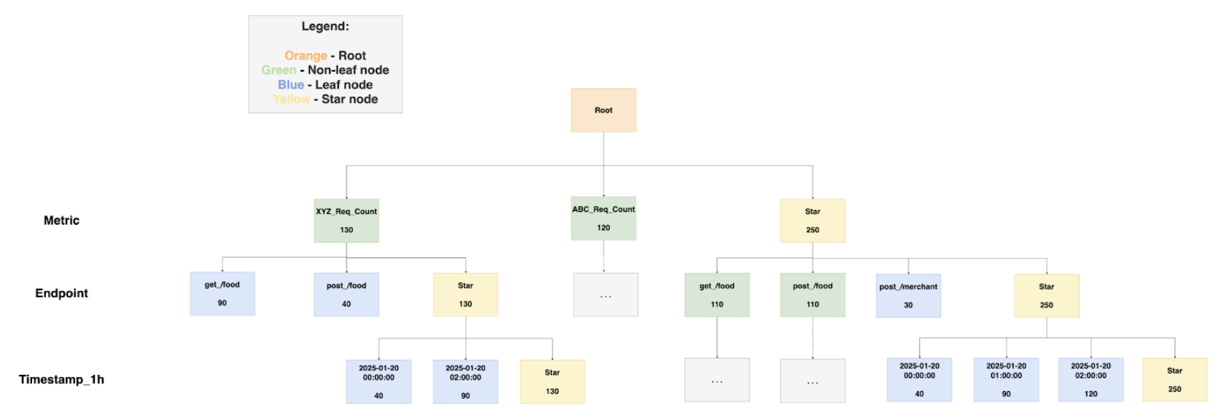
Components:

• Root node (orange): This is the starting point for traversing the tree structure.
• Leaf node (blue): These nodes contain up to a configurable number of records, denoted by T. In this configuration, maxLeafRecords is set to 1, meaning each leaf node will contain a maximum of one record.
• Non-leaf node (green): These nodes will split into child nodes if they exceed the maxLeafRecords threshold. Since maxLeafRecords is set to 1, any node with more than one record will split.
• Star-node (yellow): These nodes store pre-aggregated records by omitting the dimension used for splitting at that level. This helps in reducing the data size and improving query performance.

Example:

A practical explanation of the start-tree diagram would be to display the star-tree documents in a table format along with the sample queries used to retrieve the data.

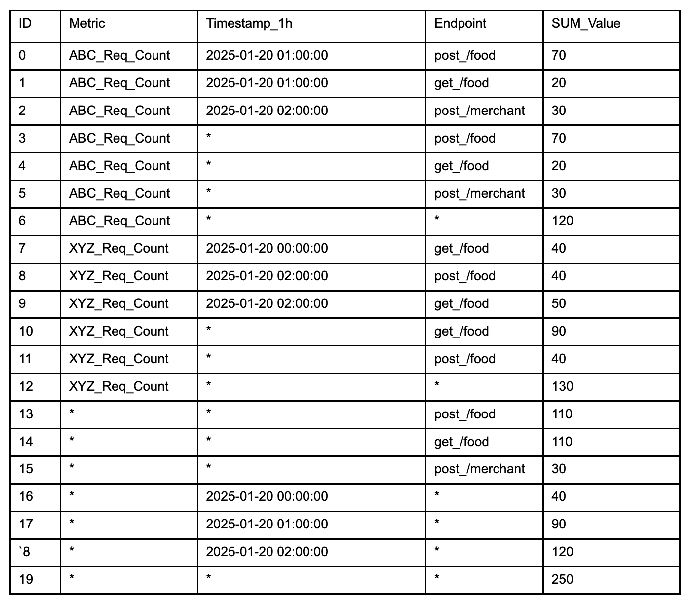
Sample queries:

Select SUM(Value) FROM Table:
With no group-by clause, select the Star-Node for all dimensions (document 19) to quickly obtain the aggregated result of 250 by processing just this document.

Select SUM(Value) FROM Table WHERE Metric = 'XYZ_Req_Count':
Select the node with XYZ_Req_Count for Metric, and the Star-Node for Endpoint and Timestamp_1h (document 12). This reduces processing to one document, returning an aggregated result of 130, instead of filtering and aggregating three documents (documents 7,8 9)

SELECT SUM(Value) FROM Table WHERE Timestamp_1h = '2025-01-20 00:00:00':
Select the Star-Node for Metric and Endpoint, and the node with '2025-01-20 00:00:00' for Timestamp_1h (document 16). This allows aggregation from a single document, yielding a result of 40.

SELECT SUM(Value) FROM Table GROUP BY Endpoint:
With a group-by on Endpoint, select the Star-Node for Metric and Timestamp_1h, and all non Star-Node for Endpoint (documents 13, 14, 15). Process one document per group to obtain the group-by results efficiently.

Comparing performance after the optimization

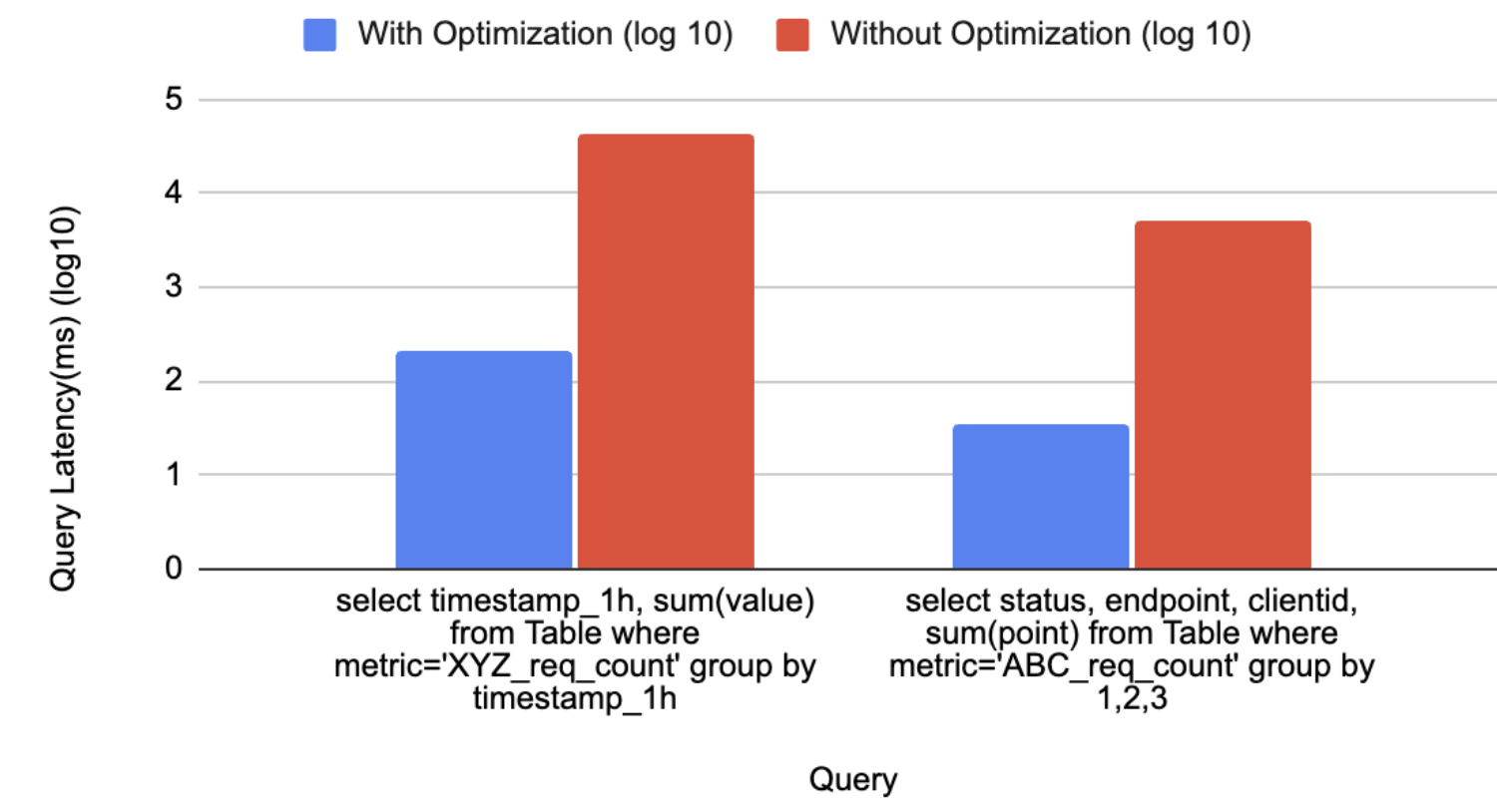
The graph above in Figure 6, provides a comparison analysis of query performance, showcasing the significant improvements achieved through the implemented optimization solutions. The query execution times are significantly reduced, as evidenced by the logarithmic scale values.

For the first query which calculates the latency for a particular aggregation interval, the log scale indicates a reduction from 4.64 to 2.32, translating to a decrease in query latency from 43,713 to 209 milliseconds.

Similarly, the second query, which aggregates the sum of the latency based on the tags for a particular metric, shows a log scale reduction from 3.71 to 1.54, with query latency improving from 5,072 to 35 milliseconds. These results underscore the efficacy of optimization in enhancing query performance, enabling faster data retrieval and processing

Tradeoffs

Star-tree indexes in Apache Pinot are designed to significantly enhance query performance by pre-computing aggregations. This approach allows for rapid query execution by utilizing pre-calculated results, rather than computing aggregations on-the-fly. However, this performance boost comes with a tradeoff in terms of storage space.

Before implementing the Star-tree index, the total storage size for 30 days of data was approximately 192GB. With the Star-tree index, this increased to 373GB, nearly doubling the storage requirements. Despite the increase in storage, the performance benefits substantially outweigh the costs associated with additional storage.

The cost impact is relatively minor. We utilize AWS gp3 EBS volumes, which roughly cost $14.48 USD monthly for the extra table (calculated as 0.08 USD x 181 GB). This cost is considered insignificant when compared to the substantial gains in query performance. Alternatively, precomputing the metrics via an ETL job is also feasible; however, it is less cost-effective due to the additional expenses required to maintain the pipeline.

The decision to use Star-tree indexes is justified by the dramatic improvement in query speed, which enhances user experience and efficiency. The modest increase in storage costs is a worthwhile investment for achieving optimal performance.

Conclusion

In conclusion, Grab’s integration of Apache Pinot as a backend solution within the Partner Gateway represents a forward-thinking strategy to meet the evolving demands of real-time analytics. Apache Pinot’s ability to deliver low-latency queries empowers our partners with immediate, actionable insights into API performance that enhances their integration experience and operational efficiency. This is crucial for partners who require rapid data access to make informed decisions and optimize their services.

The adoption of Star-tree indexing within Pinot further refines our analytics infrastructure by strategically balancing the trade-offs between query latency and storage costs. This optimization ensures Partner Gateway can support a diverse range of use cases with subsecond query latencies while maintaining high performance and reliability in service delivery reinforcing Grab’s commitment to delivering superior performance across its ecosystem.

Ultimately, the integration of Apache Pinot enhances Grab’s real-time analytics capabilities while empowering the company to drive innovation and consistently deliver exceptional service to both partners and users.

Credits to Manh Nguyen from the Coban Infrastructure Team, Michael Wengle from the Midas Team and Yuqi Wang from the DevHome team.

Join us

Grab is a leading superapp in Southeast Asia, operating across the deliveries, mobility and digital financial services sectors. Serving over 800 cities in eight Southeast Asian countries, Grab enables millions of people everyday to order food or groceries, send packages, hail a ride or taxi, pay for online purchases or access services such as lending and insurance, all through a single app. Grab was founded in 2012 with the mission to drive Southeast Asia forward by creating economic empowerment for everyone. Grab strives to serve a triple bottom line – we aim to simultaneously deliver financial performance for our shareholders and have a positive social impact, which includes economic empowerment for millions of people in the region, while mitigating our environmental footprint.

Powered by technology and driven by heart, our mission is to drive Southeast Asia forward by creating economic empowerment for everyone. If this mission speaks to you, join our team today!