Post Syndicated from Ritesh Sinha original https://aws.amazon.com/blogs/big-data/automate-data-loading-from-your-database-into-amazon-redshift-using-aws-database-migration-service-dms-aws-step-functions-and-the-redshift-data-api/

Amazon Redshift is a fast, scalable, secure, and fully managed cloud data warehouse that makes it simple and cost-effective to analyze all your data using standard SQL and your existing ETL (extract, transform, and load), business intelligence (BI), and reporting tools. Tens of thousands of customers use Amazon Redshift to process exabytes of data per day and power analytics workloads such as BI, predictive analytics, and real-time streaming analytics.

As more and more data is being generated, collected, processed, and stored in many different systems, making the data available for end-users at the right place and right time is a very important aspect for data warehouse implementation. A fully automated and highly scalable ETL process helps minimize the operational effort that you must invest in managing the regular ETL pipelines. It also provides timely refreshes of data in your data warehouse.

You can approach the data integration process in two ways:

• Full load – This method involves completely reloading all the data within a specific data warehouse table or dataset
• Incremental load – This method focuses on updating or adding only the changed or new data to the existing dataset in a data warehouse

This post discusses how to automate ingestion of source data that changes completely and has no way to track the changes. This is useful for customers who want to use this data in Amazon Redshift; some examples of such data are products and bills of materials without tracking details at the source.

We show how to build an automatic extract and load process from various relational database systems into a data warehouse for full load only. A full load is performed from SQL Server to Amazon Redshift using AWS Database Migration Service (AWS DMS). When Amazon EventBridge receives a full load completion notification from AWS DMS, ETL processes are run on Amazon Redshift to process data. AWS Step Functions is used to orchestrate this ETL pipeline. Alternatively, you could use Amazon Managed Workflows for Apache Airflow (Amazon MWAA), a managed orchestration service for Apache Airflow that makes it straightforward to set up and operate end-to-end data pipelines in the cloud.

Solution overview

The workflow consists of the following steps:

1. The solution uses an AWS DMS migration task that replicates the full load dataset from the configured SQL Server source to a target Redshift cluster in a staging area.
2. AWS DMS publishes the replicationtaskstopped event to EventBridge when the replication task is complete, which invokes an EventBridge rule.
3. EventBridge routes the event to a Step Functions state machine.
4. The state machine calls a Redshift stored procedure through the Redshift Data API, which loads the dataset from the staging area to the target production tables. With this API, you can also access Redshift data with web-based service applications, including AWS Lambda.

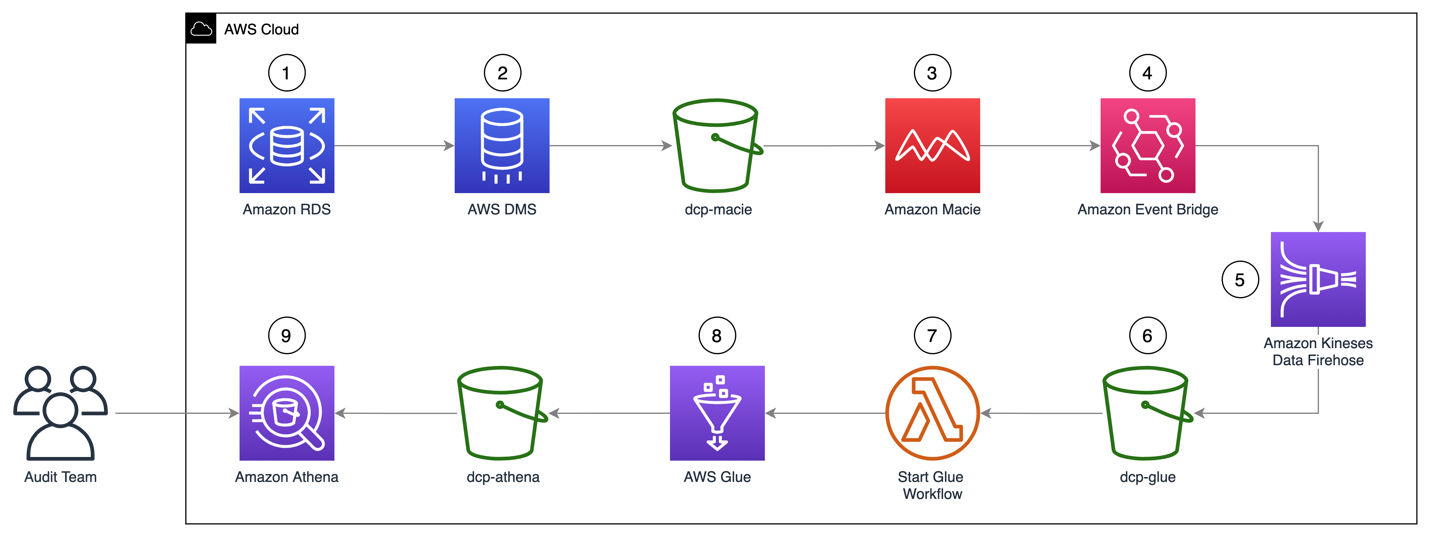
The following architecture diagram highlights the end-to-end solution using AWS services.

In the following sections, we demonstrate how to create the full load AWS DMS task, configure the ETL orchestration on Amazon Redshift, create the EventBridge rule, and test the solution.

Prerequisites

To complete this walkthrough, you must have the following prerequisites:

• An AWS account
• A SQL Server database configured as a replication source for AWS DMS
• A Redshift cluster to serve as the target database
• An AWS DMS replication instance to migrate data from source to target
• A source endpoint pointing to the SQL Server database
• A target endpoint pointing to the Redshift cluster

Create the full load AWS DMS task

Complete the following steps to set up your migration task:

1. On the AWS DMS console, choose Database migration tasks in the navigation pane.
2. Choose Create task.
3. For Task identifier, enter a name for your task, such as dms-full-dump-task.
4. Choose your replication instance.
5. Choose your source endpoint.
6. Choose your target endpoint.
7. For Migration type, choose Migrate existing data.

8. In the Table mapping section, under Selection rules, choose Add new selection rule
9. For Schema, choose Enter a schema.
10. For Schema name, enter a name (for example, dms_sample).
11. Keep the remaining settings as default and choose Create task.

The following screenshot shows your completed task on the AWS DMS console.

Create Redshift tables

Create the following tables on the Redshift cluster using the Redshift query editor:

• dbo.dim_cust – Stores customer attributes:

CREATE TABLE dbo.dim_cust (
cust_key integer ENCODE az64,
cust_id character varying(10) ENCODE lzo,
cust_name character varying(100) ENCODE lzo,
cust_city character varying(50) ENCODE lzo,
cust_rev_flg character varying(1) ENCODE lzo
)

DISTSTYLE AUTO;

• dbo.fact_sales – Stores customer sales transactions:

CREATE TABLE dbo.fact_sales (
order_number character varying(20) ENCODE lzo,
cust_key integer ENCODE az64,
order_amt numeric(18,2) ENCODE az64
)

DISTSTYLE AUTO;

• dbo.fact_sales_stg – Stores daily customer incremental sales transactions:

CREATE TABLE dbo.fact_sales_stg (
order_number character varying(20) ENCODE lzo,
cust_id character varying(10) ENCODE lzo,
order_amt numeric(18,2) ENCODE az64
)

DISTSTYLE AUTO;

Use the following INSERT statements to load sample data into the sales staging table:

insert into dbo.fact_sales_stg(order_number,cust_id,order_amt) values (100,1,200);
insert into dbo.fact_sales_stg(order_number,cust_id,order_amt) values (101,1,300);
insert into dbo.fact_sales_stg(order_number,cust_id,order_amt) values (102,2,25);
insert into dbo.fact_sales_stg(order_number,cust_id,order_amt) values (103,2,35);
insert into dbo.fact_sales_stg(order_number,cust_id,order_amt) values (104,3,80);
insert into dbo.fact_sales_stg(order_number,cust_id,order_amt) values (105,3,45);

Create the stored procedures

In the Redshift query editor, create the following stored procedures to process customer and sales transaction data:

• Sp_load_cust_dim() – This procedure compares the customer dimension with incremental customer data in staging and populates the customer dimension:

CREATE OR REPLACE PROCEDURE dbo.sp_load_cust_dim()
LANGUAGE plpgsql
AS $$
BEGIN
truncate table dbo.dim_cust;
insert into dbo.dim_cust(cust_key,cust_id,cust_name,cust_city) values (1,100,'abc','chicago');
insert into dbo.dim_cust(cust_key,cust_id,cust_name,cust_city) values (2,101,'xyz','dallas');
insert into dbo.dim_cust(cust_key,cust_id,cust_name,cust_city) values (3,102,'yrt','new york');
update dbo.dim_cust
set cust_rev_flg=case when cust_city='new york' then 'Y' else 'N' end
where cust_rev_flg is null;
END;
$$

• sp_load_fact_sales() – This procedure does the transformation for incremental order data by joining with the date dimension and customer dimension and populates the primary keys from the respective dimension tables in the final sales fact table:

CREATE OR REPLACE PROCEDURE dbo.sp_load_fact_sales()
LANGUAGE plpgsql
AS $$
BEGIN
--Process Fact Sales
insert into dbo.fact_sales
select
sales_fct.order_number,
cust.cust_key as cust_key,
sales_fct.order_amt
from dbo.fact_sales_stg sales_fct
--join to customer dim
inner join (select * from dbo.dim_cust) cust on sales_fct.cust_id=cust.cust_id;
END;
$$

Create the Step Functions state machine

Complete the following steps to create the state machine redshift-elt-load-customer-sales. This state machine is invoked as soon as the AWS DMS full load task for the customer table is complete.

1. On the Step Functions console, choose State machines in the navigation pane.
2. Choose Create state machine.
3. For Template, choose Blank.
4. On the Actions dropdown menu, choose Import definition to import the workflow definition of the state machine.

5. Open your preferred text editor and save the following code as an ASL file extension (for example, redshift-elt-load-customer-sales.ASL). Provide your Redshift cluster ID and the secret ARN for your Redshift cluster.

{
"Comment": "State Machine to process ETL for Customer Sales Transactions",
"StartAt": "Load_Customer_Dim",
"States": {
"Load_Customer_Dim": {
"Type": "Task",
"Parameters": {
"ClusterIdentifier": "redshiftcluster-abcd",
"Database": "dev",
"Sql": "call dbo.sp_load_cust_dim()",
"SecretArn": "arn:aws:secretsmanager:us-west-2:xxx:secret:rs-cluster-secret-abcd"
},
"Resource": "arn:aws:states:::aws-sdk:redshiftdata:executeStatement",
"Next": "Wait on Load_Customer_Dim"
},
"Wait on Load_Customer_Dim": {
"Type": "Wait",
"Seconds": 30,
"Next": "Check_Status_Load_Customer_Dim"
},

"Check_Status_Load_Customer_Dim": {
"Type": "Task",
"Next": "Choice",
"Parameters": {
"Id.$": "$.Id"
},

"Resource": "arn:aws:states:::aws-sdk:redshiftdata:describeStatement"
},

"Choice": {
"Type": "Choice",
"Choices": [
{
"Not": {
"Variable": "$.Status",
"StringEquals": "FINISHED"
},
"Next": "Wait on Load_Customer_Dim"
}
],
"Default": "Load_Sales_Fact"
},
"Load_Sales_Fact": {
"Type": "Task",
"End": true,
"Parameters": {
"ClusterIdentifier": "redshiftcluster-abcdef”,
"Database": "dev",
"Sql": "call dbo.sp_load_fact_sales()",
"SecretArn": "arn:aws:secretsmanager:us-west-2:xxx:secret:rs-cluster-secret-abcd"
},

"Resource": "arn:aws:states:::aws-sdk:redshiftdata:executeStatement"
}
}
}

6. Choose Choose file and upload the ASL file to create a new state machine.

7. For State machine name, enter a name for the state machine (for example, redshift-elt-load-customer-sales).
8. Choose Create.

After the successful creation of the state machine, you can verify the details as shown in the following screenshot.

The following diagram illustrates the state machine workflow.

The state machine includes the following steps:

• Load_Customer_Dim – Performs the following actions:
  • Passes the stored procedure sp_load_cust_dim to the execute-statement API to run in the Redshift cluster to load the incremental data for the customer dimension
  • Sends data back the identifier of the SQL statement to the state machine
• Wait_on_Load_Customer_Dim – Waits for at least 15 seconds
• Check_Status_Load_Customer_Dim – Invokes the Data API’s describeStatement to get the status of the API call
• is_run_Load_Customer_Dim_complete – Routes the next step of the ETL workflow depending on its status:
  • FINISHED – Passes the stored procedure Load_Sales_Fact to the execute-statement API to run in the Redshift cluster, which loads the incremental data for fact sales and populates the corresponding keys from the customer and date dimensions
  • All other statuses – Goes back to the wait_on_load_customer_dim step to wait for the SQL statements to finish

The state machine redshift-elt-load-customer-sales loads the dim_cust, fact_sales_stg, and fact_sales tables when invoked by the EventBridge rule.

As an optional step, you can set up event-based notifications on completion of the state machine to invoke any downstream actions, such as Amazon Simple Notification Service (Amazon SNS) or further ETL processes.

Create an EventBridge rule

EventBridge sends event notifications to the Step Functions state machine when the full load is complete. You can also turn event notifications on or off in EventBridge.

Complete the following steps to create the EventBridge rule:

1. On the EventBridge console, in the navigation pane, choose Rules.
2. Choose Create rule.
3. For Name, enter a name (for example, dms-test).
4. Optionally, enter a description for the rule.
5. For Event bus, choose the event bus to associate with this rule. If you want this rule to match events that come from your account, select AWS default event bus. When an AWS service in your account emits an event, it always goes to your account’s default event bus.
6. For Rule type, choose Rule with an event pattern.
7. Choose Next.
8. For Event source, choose AWS events or EventBridge partner events.
9. For Method, select Use pattern form.
10. For Event source, choose AWS services.
11. For AWS service, choose Database Migration Service.
12. For Event type, choose All Events.
13. For Event pattern, enter the following JSON expression, which looks for the REPLICATON_TASK_STOPPED status for the AWS DMS task:

{
"source": ["aws.dms"],
"detail": {
"eventId": ["DMS-EVENT-0079"],
"eventType": ["REPLICATION_TASK_STOPPED"],
"detailMessage": ["Stop Reason FULL_LOAD_ONLY_FINISHED"],
"type": ["REPLICATION_TASK"],
"category": ["StateChange"]
}
}

14. For Target type, choose AWS service.
15. For AWS service, choose Step Functions state machine.
16. For State machine name, enter redshift-elt-load-customer-sales.
17. Choose Create rule.

The following screenshot shows the details of the rule created for this post.

Test the solution

Run the task and wait for the workload to complete. This workflow moves the full volume data from the source database to the Redshift cluster.

The following screenshot shows the load statistics for the customer table full load.

AWS DMS provides notifications when an AWS DMS event occurs, for example the completion of a full load or if a replication task has stopped.

After the full load is complete, AWS DMS sends events to the default event bus for your account. The following screenshot shows an example of invoking the target Step Functions state machine using the rule you created.

We configured the Step Functions state machine as a target in EventBridge. This enables EventBridge to invoke the Step Functions workflow in response to the completion of an AWS DMS full load task.

Validate the state machine orchestration

When the entire customer sales data pipeline is complete, you may go through the entire event history for the Step Functions state machine, as shown in the following screenshots.

Limitations

The Data API and Step Functions AWS SDK integration offers a robust mechanism to build highly distributed ETL applications within minimal developer overhead. Consider the following limitations when using the Data API and Step Functions:

• Considerations when calling the Data API
• Step Functions quotas

Clean up

To avoid incurring future charges, delete the Redshift cluster, AWS DMS full load task, AWS DMS replication instance, and Step Functions state machine that you created as part of this post.

Conclusion

In this post, we demonstrated how to build an ETL orchestration for full loads from operational data stores using the Redshift Data API, EventBridge, Step Functions with AWS SDK integration, and Redshift stored procedures.

To learn more about the Data API, see Using the Amazon Redshift Data API to interact with Amazon Redshift clusters and Using the Amazon Redshift Data API.

About the authors

Ritesh Kumar Sinha is an Analytics Specialist Solutions Architect based out of San Francisco. He has helped customers build scalable data warehousing and big data solutions for over 16 years. He loves to design and build efficient end-to-end solutions on AWS. In his spare time, he loves reading, walking, and doing yoga.

Praveen Kadipikonda is a Senior Analytics Specialist Solutions Architect at AWS based out of Dallas. He helps customers build efficient, performant, and scalable analytic solutions. He has worked with building databases and data warehouse solutions for over 15 years.

Jagadish Kumar (Jag) is a Senior Specialist Solutions Architect at AWS focused on Amazon OpenSearch Service. He is deeply passionate about Data Architecture and helps customers build analytics solutions at scale on AWS.