Managing database environments demands a balance of resource efficiency and scalability. Organizations need flexible options across their entire database lifecycle, spanning development, testing, and production workloads with diverse storage and compute requirements.
To address these needs, we’re announcing four new capabilities for Amazon Relational Database Service (Amazon RDS) to help customers optimize their costs as well as improve efficiency and scalability for their Amazon RDS for Oracle and Amazon RDS for SQL Server databases. These enhancements include SQL Server Developer Edition support and expanded storage capabilities for both RDS for Oracle and RDS for SQL Server. Additionally, you can have CPU optimization options for RDS for SQL Server on M7i and R7i instances, which offer price reductions from previous generation instances and separately billed licensing fees.
Let’s explore what’s new.
SQL Server Developer Edition support SQL Server Developer Edition is now available on RDS for SQL Server, offering a free SQL Server edition that includes all the Enterprise Edition functionalities. Developer Edition is licensed specifically for non-production workloads, so you can build and test applications without incurring SQL Server licensing costs in your development and testing environments.
This release brings significant cost savings to your development and testing environments, while maintaining consistency with your production configurations. You’ll have access to all Enterprise Edition features in your development environment, making it easier to test and validate your applications. Additionally, you’ll benefit from the full suite of Amazon RDS features, including automated backups, software updates, monitoring, and encryption capabilities throughout your development process.
To get started, upload your SQL Server binary files to Amazon Simple Storage Service (Amazon S3) and use them to create your Developer Edition instance. You can migrate existing data from your Enterprise or Standard Edition instances to Developer Edition instances using built-in SQL Server backup and restore operations.
M7i/R7i instances on RDS for SQL Server with support for optimize CPU You can now use M7i and R7i instances on Amazon RDS for SQL Server to achieve several key benefits. These instances offer significant cost savings over previous generation instances. You also get improved transparency over your database costs with licensing fees and Amazon RDS DB instances costs billed separately.
RDS for SQL Server M7i/R7i instances offer up to 55% lower costs compared to previous generation instances.
Using the optimize CPU capability on these instances, you can customize the number of vCPUs on license-included RDS for SQL Server instances. This enhancement is particularly valuable for database workloads that require high memory and input/output operations per second (IOPS), but lower vCPU counts
This feature provides substantial benefits for your database operations. You can significantly reduce vCPU-based licensing costs while maintaining the same memory and IOPS performance levels your applications require. The capability supports higher memory-to-vCPU ratios and automatically disables hyperthreading while maintaining instance performance. Most importantly, you can fine-tune your CPU settings to precisely match your specific workload requirements, providing optimal resource utilization.
To get started, select SQL Server with an M7i or R7i instance type when creating a new database instance. Under Optimize CPU select Configure the number of vCPUs and set your desired vCPU count.
Additional storage volumes for RDS for Oracle and SQL Server Amazon RDS for Oracle and Amazon RDS for SQL Server now support up to 256 TiB storage size, a fourfold increase in storage size per database instance, through the addition of up to three additional storage volumes.
The additional storage volumes provide extensive flexibility in managing your database storage needs. You can configure your volumes using both io2 and gp3 volumes to create an optimal storage strategy. You can store frequently accessed data on high-performance Provisioned IOPS SSD (io2) volumes while keeping historical data on cost-effective General Purpose SSD (gp3) volumes, which balances performance and cost. For temporary storage needs, such as month-end processing or data imports, you can add storage volumes as needed. After these operations are complete, you can empty the volumes and then remove them to reduce unnecessary storage costs.
These storage volumes offer operational flexibility with zero downtime and you can add or remove additional storage volumes without interrupting your database operations. You can also scale up multiple volumes in parallel to quickly meet growing storage demands. For Multi-AZ deployments, all additional storage volumes are automatically replicated to maintain high availability.
Let me show you a quick example. I’ll add a storage volume to an existing RDS for Oracle database instance.
First, I navigate to the RDS console, then to my RDS for Oracle database instance detail page. I look under Configuration and I find the Additional storage volumes section.
You can add up to three additional storage volumes and each must be named according to a naming convention. Storage volumes can’t have the same name and you must choose between rdsdbdata2, rdsdbdata3, and rdsdbdata4. For RDS for Oracle database instances, I can add additional storage volumes to the database instance with the primary storage volume size of 200 GiB or higher.
I’m going to add two volumes, so I choose Add additional storage volume and then fill in all the required information. I choose rdsdbdata2 as the volume name and give it 12000 GiB of allocated storage with 60000 provisioned IOPS on an io2 storage type. For my second additional storage volume, rdsdbdata3, I choose to have 2000 GiB on gp3 with 15000 provisioned IOPS.
After confirmation, I wait for Amazon RDS to process my request and then my additional volumes are available.
You can also use the AWS CLI to add volumes during creation of database instances or when modifying them.
Things to know These capabilities are now available in all commercial AWS Regions and the AWS GovCloud (US) Regions where Amazon RDS for Oracle and Amazon RDS for SQL Server are offered.
This post was co-written with Frederic Haase and Julian Blau with BASF Digital Farming GmbH.
At xarvio – BASF Digital Farming, our mission is to empower farmers around the world with cutting-edge digital agronomic decision-making tools. Central to this mission is our crop optimization platform, xarvio FIELD MANAGER, which delivers actionable insights through a range of geospatial assets, including satellite imagery, drone data, and application maps from sprayers.
In this post, we show you how we built a scalable geospatial data solution on AWS to efficiently catalog, manage, and visualize both raster and vector datasets through the web. We walk you through our solution based on the SpatioTemporal Asset Catalog (STAC) specification and the open source eoAPI ecosystem, detailing the solution architecture, key technologies, and lessons learned during deployment. This builds upon a previous post on efficient satellite imagery ingestion using AWS Serverless, extending our discussion to the full lifecycle of geospatial data management at scale.
Requirements for our geospatial data solution
BASF Digital Farming’s xarvio FIELD MANAGER platform operates at exceptional scale in the geospatial data ecosystem, processing hundreds of millions of satellite images that translate into STAC items, which further decompose into billions of individual geospatial artifacts. Unlike traditional satellite data providers such as European Space Agency (ESA) who work with predictable, structured data flows, we operate in an inherently dynamic agricultural environment where we ingest near-daily satellite imagery per field from a diverse array of sensors and providers globally. Our mission to support farmers worldwide with advanced digital agronomic decision advice demands a reliable, cloud-based infrastructure capable of handling this massive data velocity and volume and applying advanced quality assurance processes including cloud detection and anomaly detection algorithms. The platform’s true value emerges through our machine learning (ML) pipelines that transform raw satellite data into actionable insights. For example, estimating accurate absolute biomass such as Leaf Area Index (LAI) helps farmers make precise, data-driven agronomic decisions that optimize crop yield and resource utilization across fields worldwide.
STAC and eoAPI ecosystem
To efficiently manage our growing archive of geospatial data, we adopted the Spatio Temporal Asset Catalog (STAC) specification, an open standard that provides a common language to describe and catalog raster and vector datasets. With STAC, we can standardize metadata across diverse sources like satellite imagery, UAV datasets, and prescription maps, making it straightforward to search, filter, and retrieve assets across our platform. We built our platform using the eoAPI ecosystem, an integrated suite of open source tools designed to handle the full lifecycle of geospatial data on the cloud. At its core is pgSTAC, which provides a performant PostGIS-backed STAC API implementation. With pgSTAC, we can index millions of STACi Items efficiently, with support for spatial, temporal, and attribute-based filtering at scale. On top of that, we use Tiles in PostGIS (TiPG) to serve tiled vector data directly from our PostGIS database. This enables real-time visualization of field boundaries, management zones, and application histories as lightweight Mapbox Vector Tiles (MVT), without requiring an external tile server. For raster assets, including satellite and drone imagery, we rely on TiTiler, a modern dynamic tile server built for Cloud Optimized GeoTIFFs (COGs). With TiTiler, we can stream imagery on-demand as WMTS or XYZ tiles, perform dynamic rendering (such as NDVI or false color composites), and integrate seamlessly into web maps and mobile apps.
Solution overview
The following architecture diagram shows how we implemented our geospatial data platform on AWS. In this section, we explain each component of the architecture and how they work together to process millions of satellite images and geospatial assets daily. The solution uses Amazon Elastic Kubernetes Service (Amazon EKS) as the core computing platform, with Amazon Simple Storage Service (Amazon S3) for storage and Amazon Relational Database Service (Amazon RDS) for metadata management. We break down the architecture into four main layers: core services, storage, database, and ingestion.
Core services layer
The solution uses an EKS cluster hosting three key services:
stac-service – Implements the STAC API specification to catalog and serve metadata for both raster and vector datasets
raster-service – Powered by TiTiler, this service dynamically renders and tiles cloud-optimized raster data (for example, COGs) for seamless integration into web and mobile maps
vector-service – Built with TiPG, this component serves vector data (for example, boundaries or application zones) as tiled MVT layers directly from the database or from Amazon S3
These services are containerized and orchestrated within Kubernetes, allowing for high availability, modular separation, and simplified continuous integration and delivery (CI/CD) workflows.
KEDA-based automatic scaling
We use Kubernetes Event-Driven Autoscaling (KEDA) to scale our platform services dynamically based on real-time workloads. With KEDA, we can scale individual pods based on precise event-driven metrics such as the STAC ingestion queue depth or visualization request load. This supports responsive performance during peak activity while maintaining lean resource usage during idle periods, aligning perfectly with our need for elasticity in a data-intensive, variable-load environment.
Geospatial asset storage layer
The platform stores all raw and processed geospatial assets in S3 buckets, optimized for performance and durability. This layer holds COGs for raster imagery and FlatGeobuf or similar formats for vector data. These formats are chosen for their support of streaming access, indexing, and cloud-based performance.
Database layer
The metadata backbone of the system is a PostgreSQL database hosted on Amazon RDS, extended with the pgSTAC plugin. This setup enables efficient indexing and querying of millions of STAC items and collections. An RDS proxy sits in front of the database, providing connection pooling and resiliency, especially under bursty or concurrent access patterns common in geospatial applications.
Ingestion layer
An independent ingestion component handles batch or streaming geospatial data inputs. This component processes satellite imagery, drone data, or prescription maps and pushes relevant metadata into the STAC API and storage assets into Amazon S3. The ingestion engine is decoupled from serving infrastructure, enabling asynchronous and large-scale data loading.
Amazon API Gateway and clients
Public access to the platform is handled through Amazon API Gateway, allowing clients—whether browser-based or mobile—to interact securely with the services. The API gateway provides a unified entrypoint and is used for applying rate limiting, authorization, and routing policies.
Solution benefits
The solution offers the following benefits:
Rapid onboarding with STAC standardization – By aligning with the STAC specification, we’ve significantly reduced the time to onboard new data domains like sprayer application maps. Compared to previous approaches in our legacy system, metadata modeling and integration are now both standardized and automated, so we can expose new geospatial data products to clients in days instead of weeks or months.
Optimized storage with COGs and Amazon S3 – Storing raster and vector assets in Amazon S3 using cloud-optimized formats (such as COGs for imagery or FlatGeobuff for vectors) reduces storage costs while enabling low-latency, streaming access. This avoids the need for preprocessing or extract, transform, and load (ETL)-heavy pipelines and simplifies client delivery.
Large-scale ingestion with a batch STAC ingestor – Our custom STAC ingestor supports both real-time and batch-mode operations. This has made it possible to onboard satellite constellations, drone imagery, and historical datasets in bulk without disrupting running services. The ingestion service uses optimized database ingestion functions, capable of ingesting thousands of items per second, providing high-throughput and reliable data integration at scale.
PostgreSQL, pgSTAC, and Amazon RDS Proxy for a scalable metadata backbone – With pgSTAC and Amazon RDS Proxy, we benefit from advanced spatial-temporal querying while making sure database connection management is handled gracefully, even under high concurrency. This combination offers reliability without compromising performance.
Scalable deployment with Amazon EKS – Hosting the solution on Amazon EKS provides full control over deployments, resource tuning, and service orchestration. Combined with automatic scaling, we dynamically adjust compute capacity based on demand, facilitating resilience and cost-efficiency.
Learnings
As part of building this solution, we learned the following:
RDS Proxy is essential for automatically scaled environments – Given our use of automatic scaling pods in Amazon EKS, we found that RDS Proxy is critical. It handles connection pooling efficiently and protects the underlying PostgreSQL database from connection exhaustion during sudden scale-up events. Without it, we encountered spiky load failures and blocked connections during high-ingest periods.
Batch STAC ingestor is a core component – Our custom STAC ingestor proved to be an indispensable piece of the system. It interfaces directly with pgSTAC to perform large-scale, automated ingestions of geospatial metadata from streams and archives. Without this tool, onboarding data providers or processing legacy imagery at scale would have been labor-intensive and error-prone.
COGs are non-negotiable – For fast, scalable visualization of large raster datasets, COGs are essential, particularly if raster datasets exceed several gigabytes. They enable efficient HTTP range requests, alleviate the need for preprocessing, and work seamlessly with TiTiler for real-time tile rendering. Non-COG formats led to noticeably slower performance and weren’t suitable for cloud-based visualization.
Serverless-compliant, optimized for Amazon EKS (for now) – Although the architecture is designed to be serverless-compatible, we opted for an Amazon EKS first approach due to the nature of our other application landscape. Components like TiTiler and TiPG benefit from persistent, memory-tuned environments that are harder to achieve in a serverless runtime. However, the solution remains modular and stateless by design, and certain subsystems (such as ingestion triggers, notifications, or monitoring) are already candidates for future serverless migration to further improve elasticity and reduce operational overhead.
Conclusion
BASF Digital Farming GmbH has successfully implemented a STAC-based geospatial data platform on Amazon EKS, enabling efficient management and visualization of satellite imagery, drone data, and application maps. This architecture helps us onboard new data sources within weeks rather than months. The new platform also processes twice as much data in a single day while cutting costs by 50%, thanks to reduced data handling through the STAC schema and the efficiencies of automatic scaling. By adopting the STAC standard, the architecture improves data discoverability, reduces search latency, and supports more efficient analytic workflows.
Organizations looking to build similar geospatial data solutions can use AWS services like Amazon EKS, Amazon S3, and Amazon RDS along with open source tools like STAC and eoAPI to create scalable, cost-effective solutions. Learn more about building containerized applications on AWS at Containers on AWS.
Unlocking powerful search capabilities for millions of items should be fast, accurate, and effortless while maintaining high relevance. Relational databases are a popular storage method for structured data, and organizations use them extensively to store their core business information. Although relational databases excel at storing and retrieving structured data, they often struggle with searching through large blocks of unstructured text and, for performance reasons, typically don’t index all columns.
In contrast, search engines such as OpenSearch index all fields, enabling rich search capabilities, including semantic search, and powerful aggregations for summarizing and analyzing numeric data. Traditionally, organizations have managed complex, inefficient, and expensive data synchronization processes, including extract, transform, and load (ETL) pipelines, to keep their search indices up to date with their databases. Those looking to enhance their applications with advanced search features need a simpler solution that can maintain search index synchronization with their databases without the overhead of managing custom data sync processes.
We are happy to announce the general availability of the integration of Amazon OpenSearch Service with Amazon Relational Database Service (Amazon RDS) and Amazon Aurora. This new integration eliminates complex data pipelines and enables near real-time data synchronization between Amazon Aurora (including Amazon Aurora MySQL-Compatible Edition and Amazon Aurora PostgreSQL-Compatible Edition) and Amazon RDS databases (including Amazon RDS for MySQL and Amazon RDS for PostgreSQL), and Amazon OpenSearch Service, unlocking advanced search capabilities such as hybrid search, ranked results, and faceted search on transactional databases. You can now deliver low-latency, high-throughput search results, live inventory updates, and personalized recommendations while focusing on creating exceptional customer experiences instead of managing data synchronization. This integration reduces the operational burden of maintaining complex ETL pipelines, reducing costs while providing instant data availability for search operations.
Amazon OpenSearch Ingestion provides near real-time data synchronization between Amazon Aurora or Amazon RDS and OpenSearch Service. Select your Aurora or RDS database, and OpenSearch Ingestion handles the rest, supporting both Aurora MySQL or RDS for MySQL (8.0 and above) and Aurora PostgreSQL or RDS for PostgreSQL (16 and above).
Solution overview
Here’s how these services work together:
Data ingestion – OpenSearch Ingestion first loads your database snapshot from Amazon Simple Storage Service (Amazon S3), where Aurora or Amazon RDS has exported the initial data. It then uses Aurora or Amazon RDS change data capture (CDC) streams to replicate further changes in near real time and indexes them into OpenSearch Service. This automated process keeps your data is consistently up to date in OpenSearch, making it readily available for search and analysis without manual intervention.
Real-time querying – OpenSearch Service offers powerful query capabilities that enable you to perform complex searches and aggregations on your data. Whether you need to analyze trends, detect anomalies, or perform search queries to return relevant results for your application, OpenSearch Service provides the tools you need.
The following diagram illustrates the solution architecture for Amazon Aurora as a source:
Getting Started
Configuring Your Database Source
Before setting up synchronization, you need to configure your source database’s logging settings. For Aurora MySQL, configure your cluster parameter group with enhanced binary log settings. For Amazon RDS, enable basic binary logging or logical replication through your instance parameter group settings. These logging configurations enable OpenSearch Ingestion to capture and replicate data changes from your database.
Before creating the view, we now explain how OpenSearch will represent this data. OpenSearch mappings define how documents and their fields are stored and indexed, similar to how a database schema defines tables and columns. The OpenSearch Ingestion pipeline uses dynamic mappings by default, automatically converting Aurora or Amazon RDS data types to appropriate OpenSearch field types. For example, database DATE fields become OpenSearch date types, and numeric fields are mapped to corresponding OpenSearch numeric types. Although you can customize these mappings using index templates, the default mappings typically handle common data types correctly, including dates, numbers, and text fields.
GET employees/_mapping
To demonstrate the integration’s ability to handle complex data relationships, we now examine how OpenSearch Ingestion handles joined data. We create a view in the sample HR database that combines information from multiple related tables into a single, searchable document in OpenSearch. This approach shows how you can transform normalized database structures into denormalized documents that are optimized for search operations.
This employee_details view combines data from multiple tables, creating a rich, denormalized representation of employee information. When replicated to OpenSearch, this view becomes a single, comprehensive document for each employee. This structure is ideal for search operations, allowing for fast and complex queries across what were originally separate tables. For example, you could easily search for employees in a specific department and country or analyze salary distributions across regions—queries that would be more complex and potentially slower in the original normalized database structure.
In the pipeline configuration shown in the following screenshot, you can check how OpenSearch Ingestion connects to the HR database. The configuration identifies the source database and the specific tables we want to replicate. While we created a view to understand the data relationships, the pipeline tracks changes from the underlying base tables (employees, departments, locations, and regions). OpenSearch Ingestion automatically maintains these relationships, which means that changes to these tables are properly reflected in your OpenSearch index, keeping your search data consistent with your source database.
In the gif shown below, you can see a demo of setting up this integration using the visual editor of OpenSearch Ingestion.
You can also specify index mapping templates to map your Aurora or Amazon RDS fields to the correct fields in your OpenSearch Service indexes.
After you configure the integration in OpenSearch Ingestion, the pipeline automatically creates indexes that you can view in OpenSearch Dashboards. OpenSearch Ingestion first triggers an automatic export of your Aurora or Amazon RDS database to Amazon S3, then loads this snapshot data from S3 into your OpenSearch cluster to create the initial indices. After this initial load, OpenSearch Ingestion continually captures changes using binary logs (binlog) for MySQL-based databases or write-ahead logs (WAL) for PostgreSQL-based databases. This way, your OpenSearch indices stay synchronized with your source database in near real time. You can view your indices in OpenSearch Dashboards by invoking:
GET _cat/indices
Example response:
Demonstrating near real time data synchronization
Consider the first five entries in the employee table:
When you make changes to your database, OpenSearch Ingestion updates Amazon OpenSearch Service with the change data. For example, the following code updates an employee’s salary:
UPDATE hr.employees SET SALARY = 26000 WHERE EMPLOYEE_ID = 100;
Amazon Aurora sends out a change notice, your OpenSearch Ingestion pipeline picks it up, and OpenSearch Ingestion sends the changed record to OpenSearch in near real time. You can verify this with an OpenSearch query:
GET employees/_search
Important details about this feature:
Monitoring– Track pipeline performance and data synchronization through CloudWatch metrics and the OpenSearch Ingestion dashboard
Limitations – Requires same-Region and same-account deployment, primary keys for optimal synchronization, and currently has no data definition language (DDL) statement support
Conclusion
Amazon Aurora or Amazon RDS integration with Amazon OpenSearch Service is now generally available in all AWS Regions where OpenSearch Ingestion is available.
To learn more, refer to the AWS documentation for Aurora or Amazon RDS integration with Amazon OpenSearch Service:
Michael Torio is an Associate Specialist Solutions Architect at AWS focused on Amazon OpenSearch Service based out of Mountain View, CA. Michael enjoys helping customers leverage cloud technologies to solve their business challenges.
Sohaib Katariwala is a Senior Specialist Solutions Architect at AWS focused on Amazon OpenSearch Service based out of Chicago, IL. His interests are in all things data and analytics. More specifically he loves to help customers use AI in their data strategy to solve modern day challenges.
Arjun Nambiar is a Product Manager with Amazon OpenSearch Service. He focuses on ingestion technologies that enable ingesting data from a wide variety of sources into Amazon OpenSearch Service at scale. Arjun is interested in large-scale distributed systems and cloud-centered technologies, and is based out of Seattle, Washington.
Well, it’s been another historic year! We’ve watched in awe as the use of real-world generative AI has changed the tech landscape, and while we at the Architecture Blog happily participated, we also made every effort to stay true to our channel’s original scope, and your readership this last year has proven that decision was the right one.
AI/ML carries itself in the top posts this year, but we’re also happy to see that foundational topics like resiliency and cost optimization are still of great interest to our audience.
(By the way, if you were hoping for more AI/ML content, head on over to our sister channel, the AWS Machine Learning Blog!).
Without further ado, here are our top posts from 2024!
In keeping with Let’s Architect! series, we have our first of three favorites for the year. This set of resources helps you apply Well-Architected standards in practice.
As I said, Let’s Architect! has a winning series, and they’ve got a finger on the pulse of the tech world. This post about machine learning showcases some of the most exciting things happening at AWS.
Figure 3. Let’s Architect
If you’re more interested in generative AI, you can also take a look at another post from 2024: Let’s Architect! GenAI
Preparedness is another common theme in this year’s favorites. Michael, John, and Saurabh are well-versed in multi-Region architecture, and they’re here to share some strategies to contain failure impact.
Figure 4. When the application experiences an impairment using S3 resources in the primary Region, it fails over to use an S3 bucket in the secondary Region.
Let’s talk cost optimization. This post about a three-tier architecture that relies on the AWS Free Tier is a must-read for anyone looking for tips to help them avoid unnecessary costs (and that’s everyone).
Figure 5. Example of a three-tier architecture on AWS
As usual, Haleh & team are pros at making sure the Well-Architected Framework is current and relevant. Take a look at the enhanced and expanded guidance in all six pillars.
One more winning post from Luca, Federica, Vittorio, and Zamira! This collection of developer resources includes new ideas in AWS Lambda, Amazon Q Developer, and Amazon DynamoDB.
Frugality AND Well-Architected? What a winning combo! This post, inspired by the 2023 re:Invent keynote, outlines the seven laws of Frugal Architecture.
And finally, our number one post of the year! Amit and Luiz showcase a customer solution with real-world applications that builds on the guidelines of other posts in this list! Well done!
Figure 10. The Pilot Light scenario for a 3-tier application that has application servers and a database deployed in two Regions
Thank you!
As always, thanks to our contributors for their dedication and desire to share, and to you, our readers! We would be nothing with you. Literally.
For other top post lists, see our Top 10 and Top 5 posts from previous years.
AWS DMS is a cloud service that makes it possible to migrate relational databases, data warehouses, NoSQL databases, and other types of data stores. You can use AWS DMS to migrate your data into the Amazon Web Services (AWS) Cloud or between combinations of cloud and on-premises setups.
Today, more than 1 million databases have been migrated using AWS Database Migration Service. AWS DMS helps you migrate your data from one database system to another. And, when migrating between different database engines, AWS DMS SC helps to convert the source database schema and procedures to the target database system.
However, although AWS DMS SC automates many steps in these migrations, certain complex database code elements still require manual intervention, which can extend migration timelines and add cost. This is particularly the case with proprietary system functions or procedures, and data type conversions, which don’t always have direct equivalents in PostgreSQL.
The new generative AI capability in AWS DMS SC is designed to address these challenges by automating some of the most time-intensive schema conversion tasks. Using large language models (LLMs) hosted on Amazon Bedrock, the new capability expands the existing conversion capabilities. It converts code snippets in the source database that were otherwise not supported by traditional rule-based techniques, including complex procedures and functions.
Generative AI–assisted code conversion helps to reduce migration costs and accelerate project timelines. Because AWS DMS SC automates more of the schema conversion process, you can focus on higher value tasks such as refining and optimizing your applications post-migration rather than manually resolving conversion gaps. Our beta customers have already experienced success with these AI-powered features in AWS DMS SC, achieving cost savings and faster migrations.
Let’s find out how it works To demonstrate the ease of using this new generative AI capability, I’ll walk through the schema conversion process in AWS DMS SC. AWS DMS SC simplifies database migration by automatically converting my source database’s structure, including tables, views, stored procedures, functions, and more, to a format compatible with my target database. Any objects that can’t be automatically converted are flagged for manual attention.
After my project is created, I select it, and on the Schema conversion tab, I choose Launch schema conversion. It takes a couple of minutes to launch the conversion tool the first time.
AWS DMS SC with generative AI is an opt-in capability. I first activate the option. On the Settings tab, I turn on Enable Generative AI feature for conversion.
Before diving into the details of the conversion, I would like to get an overall assessment of the migration complexity. I select the schema I want to migrate. Then I select Assess in the menu.
After a few minutes, a high-level Summary is available. The Action items tab has more details. I choose Export results and choose PDF to receive a report to share with my colleagues. The report is generated and available from an S3 bucket.
The summary screen shows the percentage of Database storage objects and Database code objects that can be converted by the rule-based method. That’s 100% and 57% in this example. Let’s see how the generative AI-based conversion will change that.
The PDF contains an executive summary, various statistics about the number of objects to be migrated, the feasibility of conversion with generative AI, and the complexity of the migration.
By reading the report, I learn there is no blocker detected to migrate the stored procedures. I select the stored procedure I want to migrate (PRC_AIML_DEMO6). Then, I select the Actions menu on the source database (the left one) and choose Convert.
After a minute or two, I can read the original procedure code in the left pane and the proposed migrated version on the right panel.
The summary screen has been updated. Now, it shows that 100 percent of the code can be converted automatically.
I can edit the code and make changes as required. When I’m comfortable with the proposed new version, I select the Actions menu on the target database side (the right one) and choose Apply changes.
With this new generative AI capability, AWS DMS SC can automatically convert up to 90 percent of schema objects from commercial databases to PostgreSQL.
To support your compliance requirements, this capability is initially turned off, and you can enable it as needed. If you choose to use the generative AI features in AWS DMS SC, it will flexibly decide between traditional rule-based methods and generative AI based on the complexity of the objects being converted. Customers with strict policies against generative AI can continue to rely solely on the rule-based approach, with any unconverted or partially converted objects requiring manual adjustments.
Availability and pricing This new capability is available today in the following AWS Regions: US East (Ohio, N. Virginia), US West (Oregon), and Europe (Frankfurt).
AWS DMS Schema Conversion with generative AI provides you with a faster migration pathway and helps you accelerate your transition to AWS.
To get started, visit the AWS DMS Schema Conversion documentation and learn how this generative AI capability can simplify your next database migration.
Today, we are announcing the general availability (GA) of AWS Console-to-Code that makes it easy to convert AWS console actions to reusable code. You can use AWS Console-to-Code to record your actions and workflows in the console, such as launching an Amazon Elastic Compute Cloud (Amazon EC2) instance, and review the AWS Command Line Interface (AWS CLI) commands for your console actions. With just a few clicks, Amazon Q can generate code for you using the infrastructure-as-code (IaC) format of your choice, including AWS CloudFormation template (YAML or JSON), and AWS Cloud Development Kit (AWS CDK) (TypeScript, Python or Java). This can be used as a starting point for infrastructure automation and further customized for your production workloads, included in pipelines, and more.
Since we announced the preview last year, AWS Console-to-Code has garnered positive response from customers. It has now been improved further in this GA version, because we have continued to work backwards from customer feedback.
Simplified experience – The new user experience makes it easier for customers to manage the prototyping, recording and code generation workflows.
Preview code – The launch wizards for EC2 instances and Auto Scaling groups have been updated to allow customers to generate code for these resources without actually creating them.
Advanced code generation – AWS CDK and CloudFormation code generation is powered by Amazon Q machine learning models.
Getting started with AWS Console-to-Code Let’s begin with a simple scenario of launching an Amazon EC2 instance. Start by accessing the Amazon EC2 console. Locate the AWS Console-to-Code widget on the right and choose Start recording to initiate the recording.
Now, launch an Amazon EC2 instance using the launch instance wizard in the Amazon EC2 console. After the instance is launched, choose Stop to complete the recording.
In the Recorded actions table, review the actions that were recorded. Use the Type dropdown list to filter by write actions (Write). Choose the RunInstances action. Select Copy CLI to copy the corresponding AWS CLI command.
This is the CLI command that I got from AWS Console-to-Code:
This command can be easily modified. For this example, I updated it to launch two instances (--count 2) of type t3.micro (--instance-type). This is a simplified example, but the same technique can be applied to other workflows.
I executed the command using AWS CloudShell and it worked as expected, launching two t3.micro EC2 instances:
The single-click CLI code generation experience is based on the API commands that were used when actions were executed (while launching the EC2 instance). Its interesting to note that the companion screen surfaces recorded actions as you complete them in console. And thanks to the interactive UI with start and stop functionality, its easy to clearly scope actions for prototyping.
IaC generation using AWS CDK AWS CDK is an open-source framework for defining cloud infrastructure in code and provisioning it through AWS CloudFormation. With AWS Console-to-Code, you can generate AWS CDK code (currently in Java, Python and TypeScript) for your infrastructure workflows.
Lets continue with the EC2 launch instance use case. If you haven’t done it already, in the Amazon EC2 console, locate the AWS Console-to-Code widget on the right, choose Start recording, and launch an EC2 instance. After the instance is launched, choose Stop to complete the recording and choose the RunInstances action from the Recorded actions table.
To generate AWS CDK Python code, choose the Generate CDK Python button from the dropdown list.
You can use the code as a starting point, customizing it to make it production-ready for your specific use case.
I already had the AWS CDK installed, so I created a new Python CDK project:
mkdir c2c_cdk_demo
cd c2c_cdk_demo
cdk init app --language python
Then, I plugged in the generated code in the Python CDK project. For this example, I refactored the code into a AWS CDK Stack, changed the EC2 instance type, and made other minor changes to ensure that the code was correct. I successfully deployed it using cdk deploy.
I was able to go from the console action to launch an EC2 instance and then all the way to AWS CDK to reproduce the same result.
You can also generate CloudFormation template in YAML or JSON format:
Preview code You can also directly access AWS Console-to-Code from Preview code feature in Amazon EC2 and Amazon EC2 Auto Scaling group launch experience. This means that you don’t have to actually create the resource in order to get the infrastructure code.
To try this out, follow the steps to create an Auto Scaling group using a launch template. However, instead of Create Auto Scaling group, click Preview code. You should now see the options to generate infrastructure code or copy the AWS CLI command.
Things to know Here are a few things you should consider while using AWS Console-to-Code:
Anyone can use AWS Console-to-Code to generate AWS CLI commands for their infrastructure workflows. The code generation feature for AWS CDK and CloudFormation formats has a free quota of 25 generations per month, after which you will need an Amazon Q Developer subscription.
It’s recommended that you test and verify the generated IaC code code before deployment.
At GA, AWS Console-to-Code only records actions in Amazon EC2, Amazon VPC and Amazon RDS consoles.
The Recorded actions table in AWS Console-to-Code only display actions taken during the current session within the specific browser tab, and it does not retain actions from previous sessions or other tabs. Note that refreshing the browser tab will result in the loss of all recorded actions.
It’s been an interesting week full of AWS news as usual, but also full of vibrant faces filling up the rooms in a variety of events happening this month.
Let’s start by covering some of the releases that have caught my attention this week.
Oracle Database@AWS has been announced as part of a strategic partnership between Amazon Web Services (AWS) and Oracle. This offering allows customers to access Oracle Autonomous Database and Oracle Exadata Database Service directly within AWS simplifying cloud migration for enterprise workloads. Key features include zero-ETL integration between Oracle and AWS services for real-time data analysis, enhanced security, and optimized performance for hybrid cloud environments. This collaboration addresses the growing demand for multi-cloud flexibility and efficiency. It will be available in preview later in the year with broader availability in 2025 as it expands to new Regions.
Amazon OpenSearch Service now supports version 2.15, featuring improvements in search performance, query optimization, and AI-powered application capabilities. Key updates include radial search for vector space queries, optimizations for neural sparse and hybrid search, and the ability to enable vector and hybrid search on existing indexes. Additionally, it also introduces new features like a toxicity detection guardrail and an ML inference processor for enriching ingest pipelines. Read this guide to see how you can upgrade your Amazon OpenSearch Service domain.
So simple yet so good These releases are simple in nature, but have a big impact.
AWS Resource Access Manager (RAM) now supports AWS PrivateLink – With this release, you can now securely share resources across AWS accounts with private connectivity, without exposing traffic to the public internet. This integration allows for more secure and streamlined access to shared services via VPC endpoints, improving network security and simplifying resource sharing across organizations.
AWS Network Firewall now supports AWS PrivateLink – another security quick-win, you can now securely access and manage Network Firewall resources without exposing traffic to the public internet.
AWS IAM Identity Center now enables users to customize their experience – You can set the language and visual mode preferences, including dark mode for improved readability and reduced eye strain. This update supports 12 different languages and enables users to adjust their settings for a more personalized experience when accessing AWS resources through the portal.
Others Amazon EventBridge Pipes now supports customer managed KMS keys – Amazon EventBridge Pipes now supports customer-managed keys for server-side encryption. This update allows customers to use their own AWS Key Management Service (KMS) keys to encrypt data when transferring between sources and targets, offering more control and security over sensitive event data. The feature enhances security for point-to-point integrations without the need for custom integration code. See instructions on how to configure this in the updated documentation.
Amazon SageMaker introduces sticky session routing for inference – This allows requests from the same client to be directed to the same model instance for the duration of a session improving consistency and reducing latency, particularly in real-time inference scenarios like chatbots or recommendation systems, where session-based interactions are crucial. Read about how to configure it in this documentation guide.
Events The AWS GenAI Lofts continue to pop up around the world! This week, developers in San Francisco had the opportunity to attend two very exciting events at the AWS Gen AI Loft in San Francisco including the “Generative AI on AWS” meetup last Tuesday, featuring discussions about extended reality, future AI tools, and more. Then things got playful on Thursday with the demonstration of an Amazon Bedrock-powered MineCraft bot and AI video game battles! If you’re around San Francisco before October 19th make sure to check out the schedule to see the list of events that you can join.
Make sure to check out the AWS GenAI Loft in Sao Paulo, Brazil, which opened recently, and the AWS GenAI Loft in London, which opens September 30th. You can already start registering for events before they fill up including one called “The future of development” that offers a whole day of targeted learning for developers to help them accelerate their skills.
Our AWS communities have also been very busy throwing incredible events! I was privileged to be a speaker at AWS Community Day Belfast where I got to finally meet all of the organizers of this amazing thriving community in Northern Ireland. If you haven’t been to a community day, I really recommend you check them out! You are sure to leave energized by the dedication and passion from communities leaders like Matt Coulter, Kristi Perreault, Matthew Wilson, Chloe McAteer, and their community members – not to mention the smiles all around. 🙂
Certifications If you’ve been postponing taking an AWS certification exam, now is the perfect time! Register free for the AWS Certified: Associate Challenge before December 12, 2024 and get a 50% discount voucher to take any of the following exams: AWS Certified Solutions Architect – Associate, AWS Certified Developer – Associate, AWS Certified SysOps Administrator – Associate, or AWS Certified Data Engineer – Associate. My colleague Jenna Seybold has posted a collection of study material for each exam; check it out if you’re interested.
Also, don’t forget that the brand new AWS Certified AI Practitioner exam is now available. It is in beta stage, but you can already take it. If you pass it before February 15, 2025, you get an Early Adopter badge to add to your collection.
In this blog post, we will highlight how ZS Associates used multiple AWS services to build a highly scalable, highly performant, clinical document search platform. This platform is an advanced information retrieval system engineered to assist healthcare professionals and researchers in navigating vast repositories of medical documents, medical literature, research articles, clinical guidelines, protocol documents, activity logs, and more. The goal of this search platform is to locate specific information efficiently and accurately to support clinical decision-making, research, and other healthcare-related activities by combining queries across all the different types of clinical documentation.
ZS is a management consulting and technology firm focused on transforming global healthcare. We use leading-edge analytics, data, and science to help clients make intelligent decisions. We serve clients in a wide range of industries, including pharmaceuticals, healthcare, technology, financial services, and consumer goods. We developed and host several applications for our customers on Amazon Web Services (AWS). ZS is also an AWS Advanced Consulting Partner as well as an Amazon Redshift Service Delivery Partner. As it relates to the use case in the post, ZS is a global leader in integrated evidence and strategy planning (IESP), a set of services that help pharmaceutical companies to deliver a complete and differentiated evidence package for new medicines.
ZS uses several AWS service offerings across the variety of their products, client solutions, and services. AWS services such as Amazon Neptune and Amazon OpenSearch Service form part of their data and analytics pipelines, and AWS Batch is used for long-running data and machine learning (ML) processing tasks.
Clinical data is highly connected in nature, so ZS used Neptune, a fully managed, high performance graph database service built for the cloud, as the database to capture the ontologies and taxonomies associated with the data that formed the supporting a knowledge graph. For our search requirements, We have used OpenSearch Service, an open source, distributed search and analytics suite.
About the clinical document search platform
Clinical documents comprise of a wide variety of digital records including:
Study protocols
Evidence gaps
Clinical activities
Publications
Within global biopharmaceutical companies, there are several key personas who are responsible to generate evidence for new medicines. This evidence supports decisions by payers, health technology assessments (HTAs), physicians, and patients when making treatment decisions. Evidence generation is rife with knowledge management challenges. Over the life of a pharmaceutical asset, hundreds of studies and analyses are completed, and it becomes challenging to maintain a good record of all the evidence to address incoming questions from external healthcare stakeholders such as payers, providers, physicians, and patients. Furthermore, almost none of the information associated with evidence generation activities (such as health economics and outcomes research (HEOR), real-world evidence (RWE), collaboration studies, and investigator sponsored research (ISR)) exists as structured data; instead, the richness of the evidence activities exists in protocol documents (study design) and study reports (outcomes). Therein lies the irony—teams who are in the business of knowledge generation struggle with knowledge management.
ZS unlocked new value from unstructured data for evidence generation leads by applying large language models (LLMs) and generative artificial intelligence (AI) to power advanced semantic search on evidence protocols. Now, evidence generation leads (medical affairs, HEOR, and RWE) can have a natural-language, conversational exchange and return a list of evidence activities with high relevance considering both structured data and the details of the studies from unstructured sources.
Overview of solution
The solution was designed in layers. The document processing layer supports document ingestion and orchestration. The semantic search platform (application) layer supports backend search and the user interface. Multiple different types of data sources, including media, documents, and external taxonomies, were identified as relevant for capture and processing within the semantic search platform.
Document processing solution framework layer
All components and sub-layers are orchestrated using Amazon Managed Workflows for Apache Airflow. The pipeline in Airflow is scaled automatically based on the workload using Batch. We can broadly divide layers here as shown in the following figure:
Document Processing Solution Framework Layers
Data crawling:
In the data crawling layer, documents are retrieved from a specified source SharePoint location and deposited into a designated Amazon Simple Storage Service (Amazon S3) bucket. These documents could be in variety of formats, such as PDF, Microsoft Word, and Excel, and are processed using format-specific adapters.
Data ingestion:
The data ingestion layer is the first step of the proposed framework. At this later, data from a variety of sources smoothly enters the system’s advanced processing setup. In the pipeline, the data ingestion process takes shape through a thoughtfully structured sequence of steps.
These steps include creating a unique run ID each time a pipeline is run, managing natural language processing (NLP) model versions in the versioning table, identifying document formats, and ensuring the health of NLP model services with a service health check.
The process then proceeds with the transfer of data from the input layer to the landing layer, creation of dynamic batches, and continuous tracking of document processing status throughout the run. In case of any issues, a failsafe mechanism halts the process, enabling a smooth transition to the NLP phase of the framework.
Database ingestion:
The reporting layer processes the JSON data from the feature extraction layer and converts it into CSV files. Each CSV file contains specific information extracted from dedicated sections of documents. Subsequently, the pipeline generates a triple file using the data from these CSV files, where each set of entities signifies relationships in a subject-predicate-object format. This triple file is intended for ingestion into Neptune and OpenSearch Service. In the full document embedding module, the document content is segmented into chunks, which are then transformed into embeddings using LLMs such as llama-2 and BGE. These embeddings, along with metadata such as the document ID and page number, are stored in OpenSearch Service. We use various chunking strategies to enhance text comprehension. Semantic chunking divides text into sentences, grouping them into sets, and merges similar ones based on embeddings.
Agentic chunking uses LLMs to determine context-driven chunk sizes, focusing on proposition-based division and simplifying complex sentences. Additionally, context and document aware chunking adapts chunking logic to the nature of the content for more effective processing.
NLP:
The NLP layer serves as a crucial component in extracting specific sections or entities from documents. The feature extraction stage proceeds with localization, where sections are identified within the document to narrow down the search space for further tasks like entity extraction. LLMs are used to summarize the text extracted from document sections, enhancing the efficiency of this process. Following localization, the feature extraction step involves extracting features from the identified sections using various procedures. These procedures, prioritized based on their relevance, use models like Llama-2-7b, mistral-7b, Flan-t5-xl, and Flan-T5-xxl to extract important features and entities from the document text.
The auto-mapping phase ensures consistency by mapping extracted features to standard terms present in the ontology. This is achieved through matching the embeddings of extracted features with those stored in the OpenSearch Service index. Finally, in the Document Layout Cohesion step, the output from the auto-mapping phase is adjusted to aggregate entities at the document level, providing a cohesive representation of the document’s content.
Semantic search platform application layer
This layer, shown in the following figure, uses Neptune as the graph database and OpenSearch Service as the vector engine.
Semantic search platform application layer
Amazon OpenSearch Service:
OpenSearch Service served the dual purpose of facilitating full-text search and embedding-based semantic search. The OpenSearch Service vector engine capability helped to drive Retrieval-Augmented Generation (RAG) workflows using LLMs. This helped to provide a summarized output for search after the retrieval of a relevant document for the input query. The method used for indexing embeddings was FAISS.
OpenSearch Service domain details:
Version of OpenSearch Service: 2.9
Number of nodes: 1
Instance type: r6g.2xlarge.search
Volume size: Gp3: 500gb
Number of Availability Zones: 1
Dedicated master node: Enabled
Number of Availability Zones: 3
No of master Nodes: 3
Instance type(Master Node) : r6g.large.search
To determine the nearest neighbor, we employ the Hierarchical Navigable Small World (HNSW) algorithm. We used the FAISS approximate k-NN library for indexing and searching and the Euclidean distance (L2 norm) for distance calculation between two vectors.
Amazon Neptune:
Neptune enables full-text search (FTS) through the integration with OpenSearch Service. A native streaming service for enabling FTS provided by AWS was established to replicate data from Neptune to OpenSearch Service. Based on the business use case for search, a graph model was defined. Considering the graph model, subject matter experts from the ZS domain team curated custom taxonomy capturing hierarchical flow of classes and sub-classes pertaining to clinical data. Open source taxonomies and ontologies were also identified, which would be part of the knowledge graph. Sections and entities were identified to be extracted from clinical documents. An unstructured document processing pipeline developed by ZS processed the documents in parallel and populated triples in RDF format from documents for Neptune ingestion.
The triples are created in such a way that semantically similar concepts are linked—hence creating a semantic layer for search. After the triples files are created, they’re stored in an S3 bucket. Using the Neptune Bulk Loader, we were able to load millions of triples to the graph.
Neptune ingests both structured and unstructured data, simplifying the process to retrieve content across different sources and formats. At this point, we were able to discover previously unknown relationships between the structured and unstructured data, which was then made available to the search platform. We used SPARQL query federation to return results from the enriched knowledge graph in the Neptune graph database and integrated with OpenSearch Service.
Neptune was able to automatically scale storage and compute resources to accommodate growing datasets and concurrent API calls. Presently, the application sustains approximately 3,000 daily active users. Concurrently, there is an observation of approximately 30–50 users initiating queries simultaneously within the application environment. The Neptune graph accommodates a substantial repository of approximately 4.87 million triples. The triples count is increasing because of our daily and weekly ingestion pipeline routines.
Neptune configuration:
Instance Class: db.r5d.4xlarge
Engine version: 1.2.0.1
LLMs:
Large language models (LLMs) like Llama-2, Mistral and Zephyr are used for extraction of sections and entities. Models like Flan-t5 were also used for extraction of other similar entities used in the procedures. These selected segments and entities are crucial for domain-specific searches and therefore receive higher priority in the learning-to-rank algorithm used for search.
Additionally, LLMs are used to generate a comprehensive summary of the top search results.
The LLMs are hosted on Amazon Elastic Kubernetes Service (Amazon EKS) with GPU-enabled node groups to ensure rapid inference processing. We’re using different models for different use cases. For example, to generate embeddings we deployed a BGE base model, while Mistral, Llama2, Zephyr, and others are used to extract specific medical entities, perform part extraction, and summarize search results. By using different LLMs for distinct tasks, we aim to enhance accuracy within narrow domains, thereby improving the overall relevance of the system.
Fine tuning :
Already fine-tuned models on pharma-specific documents were used. The models used were:
PharMolix/BioMedGPT-LM-7B (finetuned LLAMA-2 on medical)
emilyalsentzer/Bio_ClinicalBERT
stanford-crfm/BioMedLM
microsoft/biogpt
Re ranker, sorter, and filter stage:
Remove any stop words and special characters from the user input query to ensure a clean query. Upon pre-processing the query, create combinations of search terms by forming combinations of terms with varying n-grams. This step enriches the search scope and improves the chances of finding relevant results. For instance, if the input query is “machine learning algorithms,” generating n-grams could result in terms like “machine learning,” “learning algorithms,” and “machine learning algorithms”. Run the search terms simultaneously using the search API to access both Neptune graph and OpenSearch Service indexes. This hybrid approach broadens the search coverage, tapping into the strengths of both data sources. Specific weight is assigned to each result obtained from the data sources based on the domain’s specifications. This weight reflects the relevance and significance of the result within the context of the search query and the underlying domain. For example, a result from Neptune graph might be weighted higher if the query pertains to graph-related concepts, i.e. the search term is related directly to the subject or object of a triple, whereas a result from OpenSearch Service might be given more weightage if it aligns closely with text-based information. Documents that appear in both Neptune graph and OpenSearch Service receive the highest priority, because they likely offer comprehensive insights. Next in priority are documents exclusively sourced from the Neptune graph, followed by those solely from OpenSearch Service. This hierarchical arrangement ensures that the most relevant and comprehensive results are presented first. After factoring in these considerations, a final score is calculated for each result. Sorting the results based on their final scores ensures that the most relevant information is presented in the top n results.
Final UI
An evidence catalogue is aggregated from disparate systems. It provides a comprehensive repository of completed, ongoing and planned evidence generation activities. As evidence leads make forward-looking plans, the existing internal base of evidence is made readily available to inform decision-making.
The following video is a demonstration of an evidence catalog:
Customer impact
When completed, the solution provided the following customer benefits:
The search on multiple data source (structured and unstructured documents) enables visibility of complex hidden relationships and insights.
Clinical documents often contain a mix of structured and unstructured data. Neptune can store structured information in a graph format, while the vector database can handle unstructured data using embeddings. This integration provides a comprehensive approach to querying and analyzing diverse clinical information.
By building a knowledge graph using Neptune, you can enrich the clinical data with additional contextual information. This can include relationships between diseases, treatments, medications, and patient records, providing a more holistic view of healthcare data.
The search application helped in staying informed about the latest research, clinical developments, and competitive landscape.
This has enabled customers to make timely decisions, identify market trends, and help positioning of products based on a comprehensive understanding of the industry.
The application helped in monitoring adverse events, tracking safety signals, and ensuring that drug-related information is easily accessible and understandable, thereby supporting pharmacovigilance efforts.
The search application is currently running in production with 3000 active users.
Customer success criteria
The following success criteria were use to evaluate the solution:
Quick, high accuracy search results: The top three search results were 99% accurate with an overall latency of less than 3 seconds for users.
Identified, extracted portions of the protocol: The sections identified has a precision of 0.98 and recall of 0.87.
Accurate and relevant search results based on simple human language that answer the user’s question.
Clear UI and transparency on which portions of the aligned documents (protocol, clinical study reports, and publications) matched the text extraction.
Knowing what evidence is completed or in-process reduces redundancy in newly proposed evidence activities.
Challenges faced and learnings
We faced two main challenges in developing and deploying this solution.
Large data volume
The unstructured documents were required to be embedded completely and OpenSearch Service helped us achieve this with the right configuration. This involved deploying OpenSearch Service with master nodes and allocating sufficient storage capacity for embedding and storing unstructured document embeddings entirely. We stored up to 100 GB of embeddings in OpenSearch Service.
Inference time reduction
In the search application, it was vital that the search results were retrieved with lowest possible latency. With the hybrid graph and embedding search, this was challenging.
We addressed high latency issues by using an interconnected framework of graphs and embeddings. Each search method complemented the other, leading to optimal results. Our streamlined search approach ensures efficient queries of both the graph and the embeddings, eliminating any inefficiencies. The graph model was designed to minimize the number of hops required to navigate from one entity to another, and we improved its performance by avoiding the storage of bulky metadata. Any metadata too large for the graph was stored in OpenSearch, which served as our metadata store for graph and vector store for embeddings. Embeddings were generated using context-aware chunking of content to reduce the total embedding count and retrieval time, resulting in efficient querying with minimal inference time.
The Horizontal Pod Autoscaler (HPA) provided by Amazon EKS, intelligently adjusts pod resources based on user-demand or query loads, optimizing resource utilization and maintaining application performance during peak usage periods.
Conclusion
In this post, we described how to build an advanced information retrieval system designed to assist healthcare professionals and researchers in navigating through a diverse range of medical documents, including study protocols, evidence gaps, clinical activities, and publications. By using Amazon OpenSearch Service as a distributed search and vector database and Amazon Neptune as a knowledge graph, ZS was able to remove the undifferentiated heavy lifting associated with building and maintaining such a complex platform.
If you’re facing similar challenges in managing and searching through vast repositories of medical data, consider exploring the powerful capabilities of OpenSearch Service and Neptune. These services can help you unlock new insights and enhance your organization’s knowledge management capabilities.
About the authors
Abhishek Pan is a Sr. Specialist SA-Data working with AWS India Public sector customers. He engages with customers to define data-driven strategy, provide deep dive sessions on analytics use cases, and design scalable and performant analytical applications. He has 12 years of experience and is passionate about databases, analytics, and AI/ML. He is an avid traveler and tries to capture the world through his lens.
Gourang Harhare is a Senior Solutions Architect at AWS based in Pune, India. With a robust background in large-scale design and implementation of enterprise systems, application modernization, and cloud native architectures, he specializes in AI/ML, serverless, and container technologies. He enjoys solving complex problems and helping customer be successful on AWS. In his free time, he likes to play table tennis, enjoy trekking, or read books
Kevin Phillips is a Neptune Specialist Solutions Architect working in the UK. He has 20 years of development and solutions architectural experience, which he uses to help support and guide customers. He has been enthusiastic about evangelizing graph databases since joining the Amazon Neptune team, and is happy to talk graph with anyone who will listen.
Sandeep Varma is a principal in ZS’s Pune, India, office with over 25 years of technology consulting experience, which includes architecting and delivering innovative solutions for complex business problems leveraging AI and technology. Sandeep has been critical in driving various large-scale programs at ZS Associates. He was the founding member the Big Data Analytics Centre of Excellence in ZS and currently leads the Enterprise Service Center of Excellence. Sandeep is a thought leader and has served as chief architect of multiple large-scale enterprise big data platforms. He specializes in rapidly building high-performance teams focused on cutting-edge technologies and high-quality delivery.
Alex Turok has over 16 years of consulting experience focused on global and US biopharmaceutical companies. Alex’s expertise is in solving ambiguous, unstructured problems for commercial and medical leadership. For his clients, he seeks to drive lasting organizational change by defining the problem, identifying the strategic options, informing a decision, and outlining the transformation journey. He has worked extensively in portfolio and brand strategy, pipeline and launch strategy, integrated evidence strategy and planning, organizational design, and customer capabilities. Since joining ZS, Alex has worked across marketing, sales, medical, access, and patient services and has touched over twenty therapeutic categories, with depth in oncology, hematology, immunology and specialty therapeutics.
Moving and transforming data between databases is a common need for many organizations. Duplicating data from a production database to a lower or lateral environment and masking personally identifiable information (PII) to comply with regulations enables development, testing, and reporting without impacting critical systems or exposing sensitive customer data. However, manually anonymizing cloned information can be taxing for security and database teams.
You can use AWS Glue Studio to set up data replication and mask PII with no coding required. AWS Glue Studio visual editor provides a low-code graphic environment to build, run, and monitor extract, transform, and load (ETL) scripts. Behind the scenes, AWS Glue handles underlying resource provisioning, job monitoring, and retries. There’s no infrastructure to manage, so you can focus on rapidly building compliant data flows between key systems.
In this post, I’ll walk you through how to copy data from one Amazon Relational Database Service (Amazon RDS) for PostgreSQL database to another, while scrubbing PII along the way using AWS Glue. You will learn how to prepare a multi-account environment to access the databases from AWS Glue, and how to model an ETL data flow that automatically masks PII as part of the transfer process, so that no sensitive information will be copied to the target database in its original form. By the end, you’ll be able to rapidly build data movement pipelines between data sources and targets, that can hide PII in order to protect individual identities, without needing to write code.
Solution overview
The following diagram illustrates the solution architecture:
The solution uses AWS Glue as an ETL engine to extract data from the source Amazon RDS database. Built-in data transformations then scrub columns containing PII using pre-defined masking functions. Finally, the AWS Glue ETL job inserts privacy-protected data into the target Amazon RDS database.
This solution employs multiple AWS accounts. Having multi-account environments is an AWS best practice to help isolate and manage your applications and data. The AWS Glue account shown in the diagram is a dedicated account that facilitates the creation and management of all necessary AWS Glue resources. This solution works across a broad array of connections that AWS Glue supports, so you can centralize the orchestration in one dedicated AWS account.
It is important to highlight the following notes about this solution:
Following AWS best practices, the three AWS accounts discussed are part of an organization, but this is not mandatory for this solution to work.
This solution is suitable for use cases that don’t require real-time replication and can run on a schedule or be initiated through events.
Walkthrough
To implement this solution, this guide walks you through the following steps:
Enable connectivity from the AWS Glue account to the source and target accounts
Create AWS Glue components for the ETL job
Create and run the AWS Glue ETL job
Verify results
Prerequisites
For this walkthrough, we’re using Amazon RDS for PostgreSQL 13.14-R1. Note that the solution will work with other versions and database engines that support the same JDBC driver versions as AWS Glue. See JDBC connections for further details.
To follow along with this post, you should have the following prerequisites:
Three AWS accounts as follows:
Source account: Hosts the source Amazon RDS for PostgreSQL database. The database contains a table with sensitive information and resides within a private subnet. For future reference, record the associated virtual private cloud (VPC) ID, security group, and private subnets associated to the Amazon RDS database.
Target account: Contains the target Amazon RDS for PostgreSQL database, with the same table structure as the source table, initially empty. The database resides within a private subnet. Similarly, write down the associated VPC ID, security group ID and private subnets.
AWS Glue account: This dedicated account holds a VPC, a private subnet, and a security group. As mentioned in the AWS Glue documentation, the security group includes a self-referencing inbound rule for All TCP and TCP ports (0-65535) to allow AWS Glue to communicate with its components.
The following figure shows a self-referencing inbound rule needed on the AWS Glue account security group.
Make sure the three VPC CIDRs do not overlap with each other, as shown in the following table:
VPC
Private subnet
Source account
10.2.0.0/16
10.2.10.0/24
AWS Glue account
10.1.0.0/16
10.1.10.0/24
Target account
10.3.0.0/16
10.3.10.0/24
The VPC network attributes enableDnsHostnames and enableDnsSupport are set to true on each VPC. For details, see Using DNS with your VPC.
An Amazon Simple Storage Service (Amazon S3) endpoint on the AWS Glue account. AWS Glue requires this endpoint to store the ETL script. During the S3 endpoint set up, make sure you associate the endpoint with the route table assigned to the private subnet on the AWS Glue account. For details on creating an S3 endpoint, see Amazon VPC Endpoints for Amazon S3.
The following diagram illustrates the environment with all prerequisites:
To streamline the process of setting up the prerequisites, you can follow the directions in the README file on this GitHub repository.
Database tables
For this example, both source and target databases contain a customer table with the exact same structure. The former is prepopulated with data as shown in the following figure:
The AWS Glue ETL job you will create focuses on masking sensitive information within specific columns. These are last_name, email, phone_number, ssn and notes.
If you want to use the same table structure and data, the SQL statements are provided in the GitHub repository.
Step 1 – Enable connectivity from the AWS Glue account to the source and target accounts
When creating an AWS Glue ETL job, provide the AWS IAM role, VPC ID, subnet ID, and security groups needed for AWS Glue to access the JDBC databases. See AWS Glue: How it works for further details.
In our example, the role, groups, and other information are in the dedicated AWS Glue account. However, for AWS Glue to connect to the databases, you need to enable access to source and target databases from your AWS Glue account’s subnet and security group.
To enable access, first you inter-connect the VPCs. This can be done using VPC peering or AWS Transit Gateway. For this example, we use VPC peering. Alternatively, you can use an S3 bucket as an intermediary storage location. See Setting up network access to data stores for further details.
Follow these steps:
Peer AWS Glue account VPC with the database VPCs
Update the route tables
Update the database security groups
Peer AWS Glue account VPC with database VPCs
Complete the following steps in the AWS VPC console:
On the AWSGlueaccount, create two VPC peering connections as described in Create VPC peering connection, one for the source account VPC, and one for the target account VPC.
On the targetaccount, accept the VPC peering request as well.
On the AWSGlueaccount, enable DNS Settings on each peering connection. This allows AWS Glue to resolve the private IP address of your databases. For instructions, follow Enable DNS resolution for VPC peering connection.
After completing the preceding steps, the list of peering connections on the AWS Glue account should look like the following figure: Note that source and target account VPCs are not peered together. Connectivity between the two accounts isn’t needed.
Update subnet route tables
This step will enable traffic from the AWS Glue account VPC to the VPC subnets associate to the databases in the source and target accounts.
Complete the following steps in the AWS VPC console:
On the AWS Glue account’sroute table, for each VPC peering connection, add one route to each private subnet associated to the database. These routes enable AWS Glue to establish a connection to the databases and limit traffic from the AWS Glue account to only the subnets associated to the databases.
On the source account’sroute table of the private subnets associated to the database, add one route for the VPC peering with the AWS Glue account. This route will allow traffic back to the AWS Glue account.
Repeat step 2 on the target account’s route table.
This step is required to allow traffic from the AWS Glue account’s security group to the source and target security groups associated to the databases.
Connections enable AWS Glue to access your databases. The main benefit of creating AWS Glue connections is that connections save time by not making you have to specify all connection details every time you create a job. You can then reuse connections when creating jobs in AWS Glue Studio without having to manually enter connection details each time. This makes the job creation process more consistent and faster.
Complete these steps on the AWS Glue account:
On the AWS Glue console, choose the Data connections link on the navigation pane.
Choose Create connection and follow the instructions in the Create connection wizard:
In Choose data source, choose JDBC as data source.
In Configure connection:
For JDBC URL, enter the JDBC URL for the source database. For PostgreSQL, the syntax is:
You can find the database-endpoint on the Amazon RDS console on the source account.
Expand Network options. For VPC, Subnet and Security group, select the ones in the centralized AWS Glue account, as shown in the following figure:
In Set Properties, for Name enter Source DB connection-Postgresql.
Repeat steps 1 and 2 to create the connection to the target Amazon RDS database. Name the connection Target DB connection-Postgresql.
Now you have two connections, one for each Amazon RDS database.
Create AWS Glue crawlers
AWS Glue crawlers allow you to automate data discovery and cataloging from data sources and targets. Crawlers explore data stores and auto-generate metadata to populate the Data Catalog, registering discovered tables in the Data Catalog. This helps you to discover and work with the data to build ETL jobs.
To create a crawler for each Amazon RDS database, complete the following steps on the AWS Glue account:
On the AWS Glue console, choose Crawlers in the navigation pane.
Choose Create crawler and follow the instructions in the Add crawler wizard:
In Set crawler properties, for Name enter Source PostgreSQL database crawler.
In Chose data sources and classifiers, choose Not yet.
In Add data source, for Data source choose JDBC, as shown in the following figure:
For Connection, choose Source DB Connection - Postgresql.
For Include path, enter the path of your database including the schema. For our example, the path is sourcedb/cx/% where sourcedb is the name of the database, and cx the schema with the customer table.
In Configure security settings, choose the AWS IAM service role created a part of the prerequisites.
In Set output and scheduling, since we don’t have a database yet in the Data Catalog to store the source database metadata, choose Add database and create a database named sourcedb-postgresql.
Repeat steps 1 and 2 to create a crawler for the target database:
In Set crawler properties, for Name enter Target PostgreSQL database crawler.
In Add data source, for Connection, choose Target DB Connection-Postgresql, and for Include path enter targetdb/cx/%.
In Add database, for Name enter targetdb-postgresql.
Now you have two crawlers, one for each Amazon RDS database, as shown in the following figure:
Run the crawlers
Next, run the crawlers. When you run a crawler, the crawler connects to the designated data store and automatically populates the Data Catalog with metadata table definitions (columns, data types, partitions, and so on). This saves time over manually defining schemas.
From the Crawlers list, select both Source PostgreSQL database crawler and Target PostgreSQLdatabase crawler, and choose Run.
When finished, each crawler creates a table in the Data Catalog. These tables are the metadata representation of the customer tables.
You now have all the resources to start creating AWS Glue ETL jobs!
Step 3 – Create and run the AWS Glue ETL Job
The proposed ETL job runs four tasks:
Source data extraction – Establishes a connection to the Amazon RDS source database and extracts the data to replicate.
PII detection and scrubbing.
Data transformation – Adjusts and removes unnecessary fields.
Target data loading – Establishes a connection to the target Amazon RDS database and inserts data with masked PII.
Let’s jump into AWS Glue Studio to create the AWS Glue ETL job.
Choose Visual ETL as shown in the following figure:
Task 1 – Source data extraction
Add a node to connect to the Amazon RDS source database:
Choose AWS Glue Data Catalog from the Sources. This adds a data source node to the canvas.
On the Data source propertiespanel, select sourcedb-postgresql database and source_cx_customer table from the Data Catalog as shown in the following figure:
Task 2 – PII detection and scrubbing
To detect and mask PII, select Detect Sensitive Data node from the Transforms tab.
Let’s take a deeper look into the Transform options on the properties panel for the Detect Sensitive Data node:
First, you can choose how you want the data to be scanned. You can select Find sensitive data in each row or Find columns that contain sensitive data as shown in the following figure. Choosing the former scans all rows for comprehensive PII identification, while the latter scans a sample for PII location at lower cost.
Selecting Find sensitive data in each row allows you to specify fine-grained action overrides. If you know your data, with fine-grained actions you can exclude certain columns from detection. You can also customize the entities to detect for every column in your dataset and skip entities that you know aren’t in specific columns. This allows your jobs to be more performant by eliminating unnecessary detection calls for those entities and perform actions unique to each column and entity combination.
In our example, we know our data and we want to apply fine-grained actions to specific columns, so let’s select Find sensitive data in each row. We’ll explore fine-grained actions further below.
Next, you select the types of sensitive information to detect. Take some time to explore the three different options.
In our example, again because we know the data, let’s select Select specific patterns. For Selected patterns, choose Person’s name, Email Address, Credit Card, Social Security Number (SSN) and US Phone as shown in the following figure. Note that some patterns, such as SSNs, apply specifically to the United States and might not detect PII data for other countries. But there are available categories applicable to other countries, and you can also use regular expressions in AWS Glue Studio to create detection entities to help meet your needs.
Next, select the level of detection sensitivity. Leave the default value (High).
Next, choose the global action to take on detected entities. Select REDACT and enter **** as the Redaction Text.
Next, you can specify fine-grained actions (overrides). Overrides are optional, but in our example, we want to exclude certain columns from detection, scan certain PII entity types on specific columns only, and specify different redaction text settings for different entity types.
Choose Add to specify the fine-grained action for each entity as shown in the following figure:
Task 3 – Data transformation
When the Detect Sensitive Data node runs, it converts the id column to string type and it adds a column named DetectedEntities with PII detection metadata to the output. We don’t need to store such metadata information in the target table, and we need to convert the id column back to integer, so let’s add a Change Schema transform node to the ETL job, as shown in the following figure. This will make these changes for us.
Note: You must select the DetectedEntities Drop checkbox for the transform node to drop the added field.
Task 4 – Target data loading
The last task for the ETL job is to establish a connection to the target database and insert the data with PII masked:
Choose AWS Glue Data Catalog from the Targets. This adds a data target node to the canvas.
On the Data target properties panel, choose targetdb-postgresql and target_cx_customer, as shown in the following figure.
Save and run the ETL job
From the Job details tab, for Name, enter ETL - Replicate customer data.
For IAM Role, choose the AWS Glue role created as part of the prerequisites.
Choose Save, then choose Run.
Monitor the job until it successfully finishes from Job run monitoring on the navigation pane.
Step 4 – Verify the results
Connect to the Amazon RDS target database and verify that the replicated rows contain the scrubbed PII data, confirming sensitive information was masked properly in transit between databases as shown in the following figure:
And that’s it! With AWS Glue Studio, you can create ETL jobs to copy data between databases and transform it along the way without any coding. Try other types of sensitive information for securing your sensitive data during replication. Also try adding and combining multiple and heterogenous data sources and targets.
Clean up
To clean up the resources created:
Delete the AWS Glue ETL job, crawlers, Data Catalog databases, and connections.
Delete the VPC peering connections.
Delete the routes added to the route tables, and inbound rules added to the security groups on the three AWS accounts.
On the AWS Glue account, delete associated Amazon S3 objects. These are in the S3 bucket with aws-glue-assets-account_id-region in its name, where account-id is your AWS Glue account ID, and region is the AWS Region you used.
Delete the Amazon RDS databases you created if you no longer need them. If you used the GitHub repository, then delete the AWS CloudFormation stacks.
Conclusion
In this post, you learned how to use AWS Glue Studio to build an ETL job that copies data from one Amazon RDS database to another and automatically detects PII data and masks the data in-flight, without writing code.
By using AWS Glue for database replication, organizations can eliminate manual processes to find hidden PII and bespoke scripting to transform it by building centralized, visible data sanitization pipelines. This improves security and compliance, and speeds time-to-market for test or analytics data provisioning.
About the Author
Monica Alcalde Angel is a Senior Solutions Architect in the Financial Services, Fintech team at AWS. She works with Blockchain and Crypto AWS customers, helping them accelerate their time to value when using AWS. She lives in New York City, and outside of work, she is passionate about traveling.
Last week, AWS Heroes from around the world gathered to celebrate the 10th anniversary of the AWS Heroes program at Global AWS Heroes Summit. This program recognizes a select group of AWS experts worldwide who go above and beyond in sharing their knowledge and making an impact within developer communities.
Matt Garman, CEO of AWS and a long-time supporter of developer communities, made a special appearance for a Q&A session with the Heroes to listen to their feedback and respond to their questions.
Here’s an epic photo from the AWS Heroes Summit:
As Matt mentioned in his Linkedin post, “The developer community has been core to everything we have done since the beginning of AWS.” Thank you, Heroes, for all you do. Wishing you all a safe flight home.
Last week’s launches Here are some launches that caught my attention last week:
Announcing the July 2024 updates to Amazon Corretto — The latest updates for the Corretto distribution of OpenJDK is now available. This includes security and critical updates for the Long-Term Supported (LTS) and Feature (FR) versions.
Productionize Fine-tuned Foundation Models from SageMaker Canvas — Amazon SageMaker Canvas now allows you to deploy fine-tuned Foundation Models (FMs) to SageMaker real-time inference endpoints, making it easier to integrate generative AI capabilities into your applications outside the SageMaker Canvas workspace.
AWS Lambda now supports SnapStart for Java functions that use the ARM64 architecture — Lambda SnapStart for Java functions on ARM64 architecture delivers up to 10x faster function startup performance and up to 34% better price performance compared to x86, enabling the building of highly responsive and scalable Java applications using AWS Lambda.
Amazon QuickSight improves controls performance — Amazon QuickSight has improved the performance of controls, allowing readers to interact with them immediately without having to wait for all relevant controls to reload. This enhancement reduces the loading time experienced by readers.
Upcoming AWS events Check your calendars and sign up for upcoming AWS events:
AWS Summits — Join free online and in-person events that bring the cloud computing community together to connect, collaborate, and learn about AWS. To learn more about future AWS Summit events, visit the AWS Summit page. Register in your nearest city: AWS Summit Taipei (July 23–24), AWS Summit Mexico City (Aug. 7), and AWS Summit Sao Paulo (Aug. 15).
AWS Community Days — Join community-led conferences that feature technical discussions, workshops, and hands-on labs led by expert AWS users and industry leaders from around the world. Upcoming AWS Community Days are in Aotearoa (Aug. 15), Nigeria (Aug. 24), New York (Aug. 28), and Belfast (Sept. 6).
Life is not always happy, there are difficult times. However, we can share our joys and sufferings with those we work with. The AWS Community is no exception.
Last week’s launches Here are some launches that got my attention:
Amazon EC2 high memory U7i Instances – These instances with up to 32 TiB of DDR5 memory and 896 vCPUs are powered by custom fourth generation Intel Xeon Scalable Processors (Sapphire Rapids). These high memory instances are designed to support large, in-memory databases including SAP HANA, Oracle, and SQL Server. To learn more, visit Jeff’s blog post.
New Amazon Connect analytics data lake – You can use a single source for contact center data including contact records, agent performance, Contact Lens insights, and more — eliminating the need to build and maintain complex data pipelines. Your organization can create your own custom reports using Amazon Connect data or combine data queried from third-party sources. To learn more, visit Donnie’s blog post.
Amazon Bedrock Converse API – This API provides developers a consistent way to invoke Amazon Bedrock models removing the complexity to adjust for model-specific differences such as inference parameters. With this API, you can write a code once and use it seamlessly with different models in Amazon Bedrock. To learn more, visit Dennis’s blog post to get started.
New Document widget for PartyRock – You can build, use, and share generative AI-powered apps for fun and for boosting personal productivity, using PartyRock. Its widgets display content, accept input, connect with other widgets, and generate outputs like text, images, and chats using foundation models. You can now use new document widget to integrate text content from files and documents directly into a PartyRock app.
30 days of alarm history in Amazon CloudWatch – You can view the history of your alarm state changes for up to 30 days prior. Previously, CloudWatch provided 2 weeks of alarm history. This extended history makes it easier to observe past behavior and review incidents over a longer period of time. To learn more, visit the CloudWatch alarms documentation section.
10x faster startup time in Amazon SageMaker Canvas – You can launch SageMaker Canvas in less than a minute and get started with your visual, no-code interface for machine learning 10x faster than before. Now, all new user profiles created in existing or new SageMaker domains can experience this accelerated startup time.
Other AWS news Here are some additional news items and a Twitch show that you might find interesting:
Let us manage your relational database! – Jeff Barr ran a poll to better understand why some AWS customers still choose to host their own databases in the cloud. Working backwards, he highlights four issues that AWS managed database services address. Consider these before hosting your own database.
AWS Merch Store Spring Sale – Do you want to buy AWS branded t-shirts, hats, bags, and so on? Get 15% off on all items now through June 7th.
Upcoming AWS events Check your calendars and sign up for these AWS events:
AWS World IPv6 Day — Join us a free in-person celebration event on June 6, for technical presentations from AWS experts plus a workshop and whiteboarding session. You will learn how to get started with IPv6 and hear from customers who have started on the journey of IPv6 adoption. Check out your near city: San Francisco, Seattle, New York, London, Mumbai, Bangkok, Singapore, Kuala Lumpur, Beijing, Manila, and Sydney.
AWS Summits — Join free online and in-person events that bring the cloud computing community together to connect, collaborate, and learn about AWS. Register in your nearest city: Stockholm (June 4), Madrid (June 5), and Washington, DC (June 26–27).
AWS re:Inforce — Join us for AWS re:Inforce (June 10–12) in Philadelphia, PA. AWS re:Inforce is a learning conference focused on AWS security solutions, cloud security, compliance, and identity. Connect with the AWS teams that build the security tools and meet AWS customers to learn about their security journeys.
AWS Community Days — Join community-led conferences that feature technical discussions, workshops, and hands-on labs led by expert AWS users and industry leaders from around the world: Midwest | Columbus (June 13), Sri Lanka (June 27), Cameroon (July 13), New Zealand (August 15), Nigeria (August 24), and New York (August 28).
In the preceding scenario, neither single-user rotation nor alternating-user rotation would meet your security or compliance standards. Single-user rotation uses database user credentials in the secret to rotate itself (assuming the user has change-password permissions). Alternating-user rotation uses Amazon RDS admin credentials from another secret to create and update a _clone user credential, which means there are two valid user credentials with identical permissions.
In this post, you will learn how to implement a modified alternating-user solution that uses Amazon RDS admin user credentials to rotate database credentials while not creating an identical _clone user. This modified rotation strategy creates a short lag between when the password in the database changes and when the secret is updated. During this brief lag before the new password is updated, database calls using the old credentials might be denied. Test this in your environment to determine if the lag is within an acceptable range.
Walkthrough
In this walkthrough, you will learn how to implement the modified rotation strategy by modifying the existing alternating-user rotation template. To accomplish this, you need to complete the following:
Configure alternating-user rotation on the database credential secret for which you want to implement the modified rotation strategy.
Modify your AWS Lambda rotation function template code to implement the modified rotation strategy.
Test the modified rotation strategy on your database credential secret and verify that the secret was rotated while also not creating a _clone user.
To configure alternating-user rotation on the database credential secret
When configuring rotation for the database user secret in the Secrets Manager console, clear the checkbox for Rotate immediately when the secret is stored. The next rotation will begin on your schedule in the Rotation schedule tab. Make sure that no _clone user is created by the default alternating-user rotation code through your database’s user tables.
Figure 1: Clear the checkbox for Rotate immediately when the secret is stored
To modify your Lambda function rotation Lambda template to implement the modified rotation strategy
In the Secrets Manager console, select the Secrets menu from the left pane. Then, select the new database user secret’s name from the Secret name column.
Figure 2: Select the new database user secret
Select the Rotation tab on the Secrets page, and then choose the link under Lambda rotation function.
Figure 3: Select the Lambda rotation function
From the rotation Lambda menu, Download select Download function code.zip.
Figure 4: Select Download function code .zip from Download
Unzip the .zip file. Open the lambda_function.py file in a code editor and make the following code changes to implement the modified rotation strategy.
The following code changes show how to modify a rotation function for the MySQL alternating-user rotation code template. You must make similar changes in the CreateSecret and SetSecret steps of the alternating-user rotation code template for your database’s engine type.
To make the needed changes, remove the lines of code that are in grey italic and add the lines of code that are bold.
Consider using AWS Lambda function versions to enable reverting your Lambda function to previous iterations in case this modified rotation strategy goes wrong.
In create_secret()
The following code suggestion removes the creation of _clone-suffixed usernames.
Remove:
-- # Get the alternate username swapping between the original user and the user with _clone appended to it
-- current_dict['username'] = get_alt_username(current_dict['username'])
In set_secret()
The following code suggestions remove the creation of _clone-suffixed usernames and subsequent checks for such usernames in conditional logic.
Keep:
# Get username character limit from environment variable
username_limit = int(os.environ.get('USERNAME_CHARACTER_LIMIT', '16'))
Remove:
-- # Get the alternate username swapping between the original user and the user with _clone appended to it
-- current_dict['username'] = get_alt_username(current_dict['username'])
Keep:
# Check that the username is within correct length requirements for version
Remove:
-- if current_dict['username'].endswith('_clone') and len(current_dict['username']) > username_limit:
Add:
++ if len(current_dict[‘username’]) > username_limit:
Keep:
raise ValueError("Unable to clone user, username length with _clone appended would exceed %s character
s" % username_limit)
# Make sure the user from current and pending match
Remove:
-- if get_alt_username(current_dict['username']) != pending_dict['username']:
Add:
++ if current_dict['username'] != pending_dict['username']:
Remove:
-- def get_alt_username(current_username):
--   """Gets the alternate username for the current_username passed in
--
--   This helper function gets the username for the alternate user based on the passed in current username.
--
--   Args:
--       current_username (client): The current username
--
--   Returns:
--      AlternateUsername: Alternate username
--
--   Raises:
--      ValueError: If the new username length would exceed the maximum allowed
--
--   """
--   clone_suffix = "_clone"
--   if current_username.endswith(clone_suffix):
--       return current_username[:(len(clone_suffix) * -1)]
--   else:
--       return current_username + clone_suffix
--
The following code suggestions remove the logic of creating a new _clone user within the database, and rotates the existing user’s password.
Keep:
with conn.cursor() as cur:
Remove:
--   cur.execute("SELECT User FROM mysql.user WHERE User = %s", pending_dict['username'])
--   # Create the user if it does not exist
--   if cur.rowcount == 0:
--      cur.execute("CREATE USER %s IDENTIFIED BY %s", (pending_dict['username'], pending_dict['password']))
--
--   # Copy grants to the new user
--   cur.execute("SHOW GRANTS FOR %s", current_dict['username'])
--   for row in cur.fetchall():
--       grant = row[0].split(' TO ')
--       new_grant_escaped = grant[0].replace('%', '%%')  # % is a special character in Python format strings.
--       cur.execute(new_grant_escaped + " TO %s", (pending_dict['username'],))
Keep:
    # Get the version of MySQL
    cur.execute("SELECT VERSION()")
    ver = cur.fetchone()[0]
Remove:
--   # Copy TLS options to the new user
--   escaped_encryption_statement = get_escaped_encryption_statement(ver)
--   cur.execute("SELECT ssl_type, ssl_cipher, x509_issuer, x509_subject FROM mysql.user WHERE User = %s", current_dict['username'])
--   tls_options = cur.fetchone()
--   ssl_type = tls_options[0]
--   if not ssl_type:
--       cur.execute(escaped_encryption_statement + " NONE", pending_dict['username'])
--   elif ssl_type == "ANY":
--       cur.execute(escaped_encryption_statement + " SSL", pending_dict['username'])
--   elif ssl_type == "X509":
--       cur.execute(escaped_encryption_statement + " X509", pending_dict['username'])
--   else:
--       cur.execute(escaped_encryption_statement + " CIPHER %s AND ISSUER %s AND SUBJECT %s", (pending_dict['username'], tls_options[1], tls_options[2], tls_options[3]))
Keep:
    # Set the password for the user and commit
    password_option = get_password_option(ver)
    cur.execute("SET PASSWORD FOR %s = " + password_option, (pending_dict['username'], pending_dict['password']))
    conn.commit()
    logger.info("setSecret: Successfully set password for %s in MySQL DB for secret arn %s." % (pending_dict['username'], arn))
Re-zip the folder with the local code changes. From the rotation Lambda menu, under the Code tab, choose Upload from and select .zip file. Upload the new .zip file.
Figure 5: Use Upload from to upload the new .zip file as the Code source
To test the modified rotation strategy
During the next scheduled rotation for the new database user secret, the modified rotation code will run. To test this immediately, select the Rotation tab within the Secrets menu and choose Rotate secret immediately in the Rotation configuration section.
Figure 6: Choose Rotate secret immediately to test the new rotation strategy
To verify that the modified rotation strategy worked, verify the sign-in details in both the secret and the database itself.
To verify the Secrets Manager secret, select the Secrets menu in the Secrets Manager console and choose Retrieve secret value under the Overview tab. Verify that the username doesn’t have a _clone suffix and that there is a new password. Alternatively, make a get-secret-value call on the secret through the AWS Command Line Interface (AWS CLI) and verify the username and password details.
Figure 7: Use the secret details page for the database user secret to verify that the value of the username key is unchanged
To verify the sign-in details in the database, sign in to the database with admin credentials. Run the following database command to verify that no users with a _clone suffix exist: SELECT * FROM mysql.user;. Make sure to use the commands appropriate for your database engine type.
Also, verify that the new sign-in credentials in the secret work by signing in to the database with the credentials.
Clean up the resources
Follow the Clean up the resources section from the AWS Security Blog post used at the start of this walkthrough.
Conclusion
In this post, you’ve learned how to configure rotation of Amazon RDS database users using a modified alternating-users rotation strategy to help meet more specific security and compliance standards. The modified strategy ensures that database users don’t rotate themselves and that there are no duplicate users created in the database.
If you have feedback about this post, submit comments in the Comments section below. If you have questions about this post, start a new thread on AWS Secrets Manager re:Post or contact AWS Support.
Agents for Amazon Bedrock now supports Provisioned Throughput pricing model – As agentic applications scale, they require higher input and output model throughput compared to on-demand limits. The Provisioned Throughput pricing model makes it possible to purchase model units for the specific base model.
Amazon EC2 Inf2 instances are now available in new regions – These instances are optimized for generative AI workloads and are generally available in the Asia Pacific (Sydney), Europe (London), Europe (Paris), Europe (Stockholm), and South America (Sao Paulo) Regions.
AWS Amplify Gen 2 is now generally available – AWS Amplify offers a code-first developer experience for building full-stack apps using TypeScript and enables developers to express app requirements like the data models, business logic, and authorization rules in TypeScript. AWS Amplify Gen 2 has added a number of features since the preview, including a new Amplify console with features such as custom domains, data management, and pull request (PR) previews.
Amazon Elastic Container Registry (ECR) adds pull through cache support for GitLab Container Registry – ECR customers can create a pull through cache rule that maps an upstream registry to a namespace in their private ECR registry. Once rule is configured, images can be pulled through ECR from GitLab Container Registry. ECR automatically creates new repositories for cached images and keeps them in-sync with the upstream registry.
Getting started with Amazon Q in VS Code – Check out this excellent step-by-step guide by Rohini Gaonkar that covers installing the extension for features like code completion chat, and productivity-boosting capabilities powered by generative AI.
AWS open source news and updates – My colleague Ricardo writes about open source projects, tools, and events from the AWS Community. Check out Ricardo’s page for the latest updates.
Upcoming AWS events Check your calendars and sign up for upcoming AWS events:
AWS Summits – Join free online and in-person events that bring the cloud computing community together to connect, collaborate, and learn about AWS. Register in your nearest city: Bengaluru (May 15–16), Seoul (May 16–17), Hong Kong (May 22), Milan (May 23), Stockholm (June 4), and Madrid (June 5).
AWS re:Inforce – Explore 2.5 days of immersive cloud security learning in the age of generative AI at AWS re:Inforce, June 10–12 in Pennsylvania.
AWS Community Days – Join community-led conferences that feature technical discussions, workshops, and hands-on labs led by expert AWS users and industry leaders from around the world: Turkey (May 18), Midwest | Columbus (June 13), Sri Lanka (June 27), Cameroon (July 13), Nigeria (August 24), and New York (August 28).
This post was co-written with Luke Sudgen, Lead DevOps Engineer Post Trade, and Padraig Murphy, Solutions Architect Post Trade, from London Stock Exchange Group.
In this post, we’ll discuss some failure scenarios that were tested by London Stock Exchange Group (LSEG) Post Trade Technology teams during a chaos engineering event supported by AWS. Chaos engineering allows LSEG to simulate real-world failures in their cloud systems as part of controlled experiments. This methodology improves resilience and observability, which reduces risk and helps achieve compliance with regulators before deploying to production.
Introduction, tooling, and methodology
As a heavily regulated provider of global financial markets infrastructure, LSEG is always looking for opportunities to enhance workload resilience. LSEG and AWS teamed up to organize and run a 3-day AWS Experience-Based Acceleration (EBA) event to perform chaos engineering experiments against key workloads. The event was sponsored and led by the architecture function and included cross-functional Post Trade technical teams across various workstreams. The experiments were run using AWS Fault Injection Service (FIS) following the experiment methodology described in the Verify the resilience of your workloads using Chaos Engineering blog post.
Resilience of modern distributed cloud systems can be continuously improved through reviewing workload architectures and recovery, assessing standard operating procedures (SOPs), and building SOP alerts and recovery automations. AWS Resilience Hub provides a comprehensive tooling suite to get started on these activities.
Another key activity to validate and enhance your resilience posture is chaos engineering, a methodology that induces controlled chaos into customer systems through real-world controlled experiments. Chaos engineering helps customers create real-world failure conditions that can uncover hidden bugs, monitor blind spots, and manage bottlenecks that are difficult to find in distributed systems. This makes it a very useful tool in regulated industries such as financial services.
Architectural overview
The architectural diagram in Figure 1 comprises a three-tier application deployed in virtual private clouds (VPCs) with a multi-AZ setup.
Figure 1. Chaos engineering pattern for hybrid architecture (3-tier application)
Operating within a public subnet, the web application creates a hybrid architecture by using an Amazon Elastic Compute Cloud (Amazon EC2) Auto Scaling group and connecting to an Amazon Relational Database Service (Amazon RDS) database that’s located in a private subnet and connected with on-premises services. Additionally, a number of internal services are hosted in a separate VPC, housed within containers. FIS provides a controlled environment to validate the robustness of the architecture against various failure scenarios, such as:
Amazon EC2 instance failure that causes the application or container pod on the machine to also fail
The objective of this use case is to evaluate the resilience of the application or container pod running on Amazon EC2 instances and identify how the system can adapt itself and continue functioning during unexpected disruptions or instability of an instance. You can use aws:ec2:stop-instances or aws:ec2:terminate-instances FIS actions to mimic different EC2 instance failure modes. The response of running containers to the different instance failures was also assessed. If you’re running containers within a managed AWS service such as Amazon Elastic Container Service (Amazon ECS) or Amazon Elastic Kubernetes Service (Amazon EKS), you can use FIS failure scenarios for ECS tasks and EKS pods.
Amazon RDS failure
RDS failure is another common scenario you can use to identify and troubleshoot database managed service failures from failovers and node reboots at a large scale. FIS can be used to inject reboot/failover failure conditions into the managed RDS instances to understand the bottlenecks and issues from disaster failovers, sync failures, and other database-related problems.
Severe network latency degradation
Network latency degradation injects latency in the network interface that connects two systems. This helps you understand how these systems handle a data transfer delay and your operational response readiness (alerts, metrics, and correction). This FIS action (aws:ssm:send-command/AWSFIS-Run-Network-Latency) uses the Linux traffic control (tc) utility.
Network connectivity disruption
Connectivity issues like traffic disruption or other network issues can be simulated with FIS network actions. FIS supports the aws:network:disrupt-connectivity action to test your application’s resilience in the event of total or partial connectivity loss within its subnet, as well as disruption (including cross-Region) with other AWS networking components such as route tables or AWS Transit Gateway.
Amazon EBS volume failure (IOPS pause)
Disk failure is a problematic issue in real-time operations-based systems. It can lead to transactions failing due to I/O failures or storage failure during peak activity in heavy workloads. The EBS volume failure actions test system performance under different disk failure scenarios. FIS supports the aws:ebs:pause-volume-io action to pause I/O operations on target EBS volumes, as well as other failure modes. The target volumes must be in the same Availability Zone and must be attached to instances built on the AWS Nitro System.
Outcomes and conclusion
Following the experiment, the teams from LSEG successfully identified a series of architectural improvements to reduce application recovery time and enhance metric granularity and alerting. As a second tangible output, the teams now have a reusable chaos engineering methodology and toolset. Running regular in-person cross-functional events is a great way to implement a chaos engineering practice in your organization.
You can start your resilience journey on AWS today with AWS Resilience Hub.
Customers across industries today are looking to use data to their competitive advantage and increase revenue and customer engagement by implementing near real time analytics use cases like personalization strategies, fraud detection, inventory monitoring, and many more. There are two broad approaches to analyzing operational data for these use cases:
Analyze the data in-place in the operational database (such as read replicas, federated query, and analytics accelerators)
Move the data to a data store optimized for running use case-specific queries such as a data warehouse
The zero-ETL integration is focused on simplifying the latter approach.
The extract, transform, and load (ETL) process has been a common pattern for moving data from an operational database to an analytics data warehouse. ELT is where the extracted data is loaded as is into the target first and then transformed. ETL and ELT pipelines can be expensive to build and complex to manage. With multiple touchpoints, intermittent errors in ETL and ELT pipelines can lead to long delays, leaving data warehouse applications with stale or missing data, further leading to missed business opportunities.
Alternatively, solutions that analyze data in-place may work great for accelerating queries on a single database, but such solutions aren’t able to aggregate data from multiple operational databases for customers that need to run unified analytics.
Zero-ETL
Unlike the traditional systems where data is siloed in one database and the user has to make a trade-off between unified analysis and performance, data engineers can now replicate data from multiple RDS for MySQL databases into a single Redshift data warehouse to derive holistic insights across many applications or partitions. Updates in transactional databases are automatically and continuously propagated to Amazon Redshift so data engineers have the most recent information in near real time. There is no infrastructure to manage and the integration can automatically scale up and down based on the data volume.
At AWS, we have been making steady progress towards bringing our zero-ETL vision to life. The following sources are currently supported for zero-ETL integrations:
When you create a zero-ETL integration for Amazon Redshift, you continue to pay for underlying source database and target Redshift database usage. Refer to Zero-ETL integration costs (Preview) for further details.
With zero-ETL integration with Amazon Redshift, the integration replicates data from the source database into the target data warehouse. The data becomes available in Amazon Redshift within seconds, allowing you to use the analytics features of Amazon Redshift and capabilities like data sharing, workload optimization autonomics, concurrency scaling, machine learning, and many more. You can continue with your transaction processing on Amazon RDS or Amazon Aurora while simultaneously using Amazon Redshift for analytics workloads such as reporting and dashboards.
The following diagram illustrates this architecture.
Solution overview
Let’s consider TICKIT, a fictional website where users buy and sell tickets online for sporting events, shows, and concerts. The transactional data from this website is loaded into an Amazon RDS for MySQL 8.0.28 (or higher version) database. The company’s business analysts want to generate metrics to identify ticket movement over time, success rates for sellers, and the best-selling events, venues, and seasons. They would like to get these metrics in near real time using a zero-ETL integration.
The integration is set up between Amazon RDS for MySQL (source) and Amazon Redshift (destination). The transactional data from the source gets refreshed in near real time on the destination, which processes analytical queries.
You can use either the serverless option or an encrypted RA3 cluster for Amazon Redshift. For this post, we use a provisioned RDS database and a Redshift provisioned data warehouse.
The following diagram illustrates the high-level architecture.
The following are the steps needed to set up zero-ETL integration. These steps can be done automatically by the zero-ETL wizard, but you will require a restart if the wizard changes the setting for Amazon RDS or Amazon Redshift. You could do these steps manually, if not already configured, and perform the restarts at your convenience. For the complete getting started guides, refer to Working with Amazon RDS zero-ETL integrations with Amazon Redshift (preview) and Working with zero-ETL integrations.
Configure the RDS for MySQL source with a custom DB parameter group.
Configure the Redshift cluster to enable case-sensitive identifiers.
Configure the required permissions.
Create the zero-ETL integration.
Create a database from the integration in Amazon Redshift.
Configure the RDS for MySQL source with a customized DB parameter group
To create an RDS for MySQL database, complete the following steps:
On the Amazon RDS console, create a DB parameter group called zero-etl-custom-pg.
Zero-ETL integration works by using binary logs (binlogs) generated by MySQL database. To enable binlogs on Amazon RDS for MySQL, a specific set of parameters must be enabled.
Set the following binlog cluster parameter settings:
binlog_format = ROW
binlog_row_image = FULL
binlog_checksum = NONE
In addition, make sure that the binlog_row_value_options parameter is not set to PARTIAL_JSON. By default, this parameter is not set.
Choose Databases in the navigation pane, then choose Create database.
For Engine Version, choose MySQL 8.0.28 (or higher).
For Templates, select Production.
For Availability and durability, select either Multi-AZ DB instance or Single DB instance (Multi-AZ DB clusters are not supported, as of this writing).
For DB instance identifier, enter zero-etl-source-rms.
Under Instance configuration, select Memory optimized classes and choose the instance db.r6g.large, which should be sufficient for TICKIT use case.
Under Additional configuration, for DB cluster parameter group, choose the parameter group you created earlier (zero-etl-custom-pg).
Choose Create database.
In a couple of minutes, it should spin up an RDS for MySQL database as the source for zero-ETL integration.
Configure the Redshift destination
After you create your source DB cluster, you must create and configure a target data warehouse in Amazon Redshift. The data warehouse must meet the following requirements:
At the top of you console window, you will see a Try new Amazon Redshift features in preview banner.
Choose Create preview cluster.
For Preview track, chose preview_2023.
For Node type, choose one of the supported node types (for this post, we use ra3.xlplus).
Under Additional configurations, expand Database configurations.
For Parameter groups, choose zero-etl-rms.
For Encryption, select Use AWS Key Management Service.
Choose Create cluster.
The cluster should become Available in a few minutes.
Navigate to the namespace zero-etl-target-rs-ns and choose the Resource policy tab.
Choose Add authorized principals.
Enter either the Amazon Resource Name (ARN) of the AWS user or role, or the AWS account ID (IAM principals) that are allowed to create integrations.
An account ID is stored as an ARN with root user.
In the Authorized integration sources section, choose Add authorized integration source to add the ARN of the RDS for MySQL DB instance that’s the data source for the zero-ETL integration.
You can find this value by going to the Amazon RDS console and navigating to the Configuration tab of the zero-etl-source-rms DB instance.
Your resource policy should resemble the following screenshot.
Configure required permissions
To create a zero-ETL integration, your user or role must have an attached identity-based policy with the appropriate AWS Identity and Access Management (IAM) permissions. An AWS account owner can configure required permissions for users or roles who may create zero-ETL integrations. The sample policy allows the associated principal to perform the following actions:
Create zero-ETL integrations for the source RDS for MySQL DB instance.
View and delete all zero-ETL integrations.
Create inbound integrations into the target data warehouse. This permission is not required if the same account owns the Redshift data warehouse and this account is an authorized principal for that data warehouse. Also note that Amazon Redshift has a different ARN format for provisioned and serverless clusters:
Attach the policy you created to your IAM user or role permissions.
Create the zero-ETL integration
To create the zero-ETL integration, complete the following steps:
On the Amazon RDS console, choose Zero-ETL integrations in the navigation pane.
Choose Create zero-ETL integration.
For Integration identifier, enter a name, for example zero-etl-demo.
For Source database, choose Browse RDS databases and choose the source cluster zero-etl-source-rms.
Choose Next.
Under Target, for Amazon Redshift data warehouse, choose Browse Redshift data warehouses and choose the Redshift data warehouse (zero-etl-target-rs).
Choose Next.
Add tags and encryption, if applicable.
Choose Next.
Verify the integration name, source, target, and other settings.
Choose Create zero-ETL integration.
You can choose the integration to view the details and monitor its progress. It took about 30 minutes for the status to change from Creating to Active.
The time will vary depending on the size of your dataset in the source.
Create a database from the integration in Amazon Redshift
To create your database from the zero-ETL integration, complete the following steps:
On the Amazon Redshift console, choose Clusters in the navigation pane.
Open the zero-etl-target-rs cluster.
Choose Query data to open the query editor v2.
Connect to the Redshift data warehouse by choosing Save.
Obtain the integration_id from the svv_integration system table:
select integration_id from svv_integration; -- copy this result, use in the next sql
Use the integration_id from the previous step to create a new database from the integration:
CREATE DATABASE zetl_source FROM INTEGRATION '<result from above>';
The integration is now complete, and an entire snapshot of the source will reflect as is in the destination. Ongoing changes will be synced in near real time.
Analyze the near real time transactional data
Now we can run analytics on TICKIT’s operational data.
Populate the source TICKIT data
To populate the source data, complete the following steps:
Copy the CSV input data files into a local directory. The following is an example command:
Connect to your RDS for MySQL cluster and create a database or schema for the TICKIT data model, verify that the tables in that schema have a primary key, and initiate the load process:
mysql -h <rds_db_instance_endpoint> -u admin -p password --local-infile=1
Load the data from local files using the LOAD DATA command.
The following is an example. Note that the input CSV file is broken into several files. This command must be run for every file if you would like to load all data. For demo purposes, a partial data load should work as well.
Analyze the source TICKIT data in the destination
On the Amazon Redshift console, open the query editor v2 using the database you created as part of the integration setup. Use the following code to validate the seed or CDC activity:
SELECT * FROM SYS_INTEGRATION_ACTIVITY ORDER BY last_commit_timestamp DESC;
You can now apply your business logic for transformations directly on the data that has been replicated to the data warehouse. You can also use performance optimization techniques like creating a Redshift materialized view that joins the replicated tables and other local tables to improve query performance for your analytical queries.
Monitoring
You can query the following system views and tables in Amazon Redshift to get information about your zero-ETL integrations with Amazon Redshift:
SVV_INTEGRATION – Provides configuration details for your integrations
To view the integration-related metrics published to Amazon CloudWatch, open the Amazon Redshift console. Choose Zero-ETL integrations in the navigation pane and choose the integration to display activity metrics.
Available metrics on the Amazon Redshift console are integration metrics and table statistics, with table statistics providing details of each table replicated from Amazon RDS for MySQL to Amazon Redshift.
Integration metrics contain table replication success and failure counts and lag details.
Manual resyncs
The zero-ETL integration will automatically initiate a resync if a table sync state shows as failed or resync required. But in case the auto resync fails, you can initiate a resync at table-level granularity:
ALTER DATABASE zetl_source INTEGRATION REFRESH TABLES tbl1, tbl2;
A table can enter a failed state for multiple reasons:
The primary key was removed from the table. In such cases, you need to re-add the primary key and perform the previously mentioned ALTER command.
An invalid value is encountered during replication or a new column is added to the table with an unsupported data type. In such cases, you need to remove the column with the unsupported data type and perform the previously mentioned ALTER command.
An internal error, in rare cases, can cause table failure. The ALTER command should fix it.
Clean up
When you delete a zero-ETL integration, your transactional data isn’t deleted from the source RDS or the target Redshift databases, but Amazon RDS doesn’t send any new changes to Amazon Redshift.
To delete a zero-ETL integration, complete the following steps:
On the Amazon RDS console, choose Zero-ETL integrations in the navigation pane.
Select the zero-ETL integration that you want to delete and choose Delete.
To confirm the deletion, choose Delete.
Conclusion
In this post, we showed you how to set up a zero-ETL integration from Amazon RDS for MySQL to Amazon Redshift. This minimizes the need to maintain complex data pipelines and enables near real time analytics on transactional and operational data.
Milind Oke is a senior Redshift specialist solutions architect who has worked at Amazon Web Services for three years. He is an AWS-certified SA Associate, Security Specialty and Analytics Specialty certification holder, based out of Queens, New York.
Aditya Samant is a relational database industry veteran with over 2 decades of experience working with commercial and open-source databases. He currently works at Amazon Web Services as a Principal Database Specialist Solutions Architect. In his role, he spends time working with customers designing scalable, secure and robust cloud native architectures. Aditya works closely with the service teams and collaborates on designing and delivery of the new features for Amazon’s managed databases.
Today, I am pleased to announce the availability of Provisioned IOPS (PIOPS) io2 Block Express storage volumes for all database engines in Amazon Relational Database Service (Amazon RDS). Amazon RDS provides you the flexibility to choose between different storage types depending on the performance requirements of your database workload. io2 Block Express volumes are designed for critical database workloads that require high performance and high throughput at low latency.
Lower latency and higher availability for I/O intensive workloads With io2 Block Express volumes, your database workloads will benefit from consistent sub-millisecond latency, enhanced durability to 99.999 percent over io1 volumes, and drive 20x more IOPS from provisioned storage (up to 1,000 IOPS per GB) at the same price as io1. You can upgrade from io1 volumes to io2 Block Express volumes without any downtime, significantly improving the performance and reliability of your applications without increasing storage cost.
“We migrated all of our primary Amazon RDS instances to io2 Block Express within 2 weeks,” said Samir Goel, Director of Engineering at Figma, a leading platform for teams that design and build digital products. “Io2 Block Express has had a profound impact on the availability of the database layer at Figma. We have deeply appreciated the consistency of performance with io2 Block Express — in our observations, the latency variability has been under 0.1ms.”
io2 Block Express volumes support up to 64 TiB of storage, up to 256,000 Provisioned IOPS, and a maximum throughput of 4,000 MiB/s. The throughput of io2 Block Express volumes varies based on the amount of provisioned IOPS and volume storage size. Here is the range for each database engine and storage size:
Database engine
Storage size
Provisioned IOPS
Maximum throughput
Db2, MariaDB, MySQL, and PostgreSQL
Between 100 and 65,536 GiB
1,000–256,000 IOPS
4,000 MiB/s
Oracle
Between 100 and 199 GiB
1,000–199,000 IOPS
4,000 MiB/s
Oracle
Between 200 and 65,536 GiB
1,000–256,000 IOPS
4,000 MiB/s
SQL Server
Between 20 and 16,384 GiB
1,000–64,000 IOPS
4,000 MiB/s
Getting started with io2 Block Express in Amazon RDS You can use the Amazon RDS console to create a new RDS instance configured with an io2 Block Express volume or modify an existing instance with io1, gp2, or gp3 volumes.
Here’s how you would create an Amazon RDS for PostgreSQL instance with io2 Block Express volume.
Start with the basic information such as engine and version. Then, choose Provisioned IOPS SDD (io2) from the Storage type options:
Use the following AWS CLI command to create a new RDS instance with io2 Block Express volume:
io2 Block Express volumes are available on all RDS databases using AWS Nitro System instances.
io2 Block Express volumes support an IOPS to allocated storage ratio of 1000:1. As an example, With an RDS for PostgreSQL instance, the maximum IOPS can be provisioned with volumes 256 GiB and larger (1,000 IOPS × 256 GiB = 256,000 IOPS).
For DB instances not based on the AWS Nitro System, the ratio of IOPS to allocated storage is 500:1. In this case, maximum IOPS can be achieved with 512 GiB volume (500 IOPS x 512 GiB = 256,000 IOPS).
Available now Amazon RDS io2 Block Express storage volumes are supported for all RDS database engines and are available in US East (Ohio, N. Virginia), US West (N. California, Oregon), Asia Pacific (Hong Kong, Mumbai, Osaka, Seoul, Singapore, Sydney, Tokyo), Canada (Central), Europe (Frankfurt, Ireland, London, Stockholm), and Middle East (Bahrain) Regions.
In terms of pricing and billing, io1 volumes and io2 Block Express storage volumes are billed at the same rate. For more information, see the Amazon RDS pricing page.
Learn more by reading about Provisioned IOPS SSD storage in the Amazon RDS User Guide.
Happy New Year! Cloud technologies, machine learning, and generative AI have become more accessible, impacting nearly every aspect of our lives. Amazon CTO Dr. Werner Vogels offers four tech predictions for 2024 and beyond:
Generative AI becomes culturally aware
FemTech finally takes off
AI assistants redefine developer productivity
Education evolves to match the speed of technology
To hear insights from AWS and industry thought leaders, grow your skills, and get inspired, watch AWS re:Invent 2023 videos on demand for keynotes, innovation talks, breakout sessions, and AWS Hero guide playlists.
Launches from the last few weeks Since our last week in review on December 18, 2023, I’d like to highlight some launches from year end, as well as last week:
New AWS Canada West (Calgary) Region – We are opening a new and second Region and in Canada, AWS Canada West (Calgary). At the end of 2023, AWS had 33 AWS Regions and 105 Availability Zones (AZs) globally. We preannounced 12 additional AZs in four future Regions in Malaysia, New Zealand, Thailand, and the AWS European Sovereign Cloud. We will share more information on these Regions in 2024. Please stay tuned.
DNS over HTTPS in Amazon Route 53 Resolver – You can use the DNS over HTTPS (DoH) protocol for both inbound and outbound Route 53 Resolver endpoints. As the name suggests, DoH supports HTTP or HTTP/2 over TLS to encrypt the data exchanged for Domain Name System (DNS) resolutions.
Automatic enrollment to Amazon RDS Extended Support – Your MySQL 5.7 and PostgreSQL 11 database instances running on Amazon Aurora and Amazon RDS will be automatically enrolled into Amazon RDS Extended Support starting on February 29, 2024. You can have more control over when you want to upgrade the major version of your database after the community end of life (EoL).
New Amazon CloudWatch Network Monitor – This is a new feature of Amazon CloudWatch that helps monitor network availability and performance between AWS and your on-premises environments. Network Monitor needs zero manual instrumentation and gives you access to real-time network visibility to proactively and quickly identify issues within the AWS network and your own hybrid environment. For more information, read Monitor hybrid connectivity with Amazon CloudWatch Network Monitor.
New WordPress setup on Amazon Lightsail– Set up your WordPress website on Amazon Lightsail with the new workflow to eliminate complexity and time spent configuring your website. The workflow allows you to complete all the necessary steps, including setting up a Secure Sockets Layer (SSL) certificate to secure your website with HTTPS.
Other AWS News Here are some other news items that you may find interesting in the new year:
Book recommendations for AWS customer executives – Plan for the new year and catch up on what others are doing and thinking. AWS Enterprise Strategy team recommends what books are most important for our AWS customer executives to read.
Best practices for scaling AWS CDK adoption with Platform Engineering – A recent evolution in DevOps is the introduction of platform engineering teams to build services, toolchains, and documentation to support workload teams. This blog post introduces strategies and best practices for accelerating CDK adoption within your organization. You can learn how to scale the lessons learned from the pilot project across your organization through platform engineering.
Upcoming AWS Events Check your calendars and sign up for these AWS events in the new year:
AWS at CES 2024 (January 9-12) – AWS will be representing some of the latest cloud services and solutions that are purpose built for the automotive, mobility, transportation, and manufacturing industries. Join us to learn about the latest cloud capabilities across generative AI, software define vehicles, product engineering, sustainability, new digital customer experiences, connected mobility, autonomous driving, and so much more in Amazon Experience Area.
APJ Builders Online Series (January 18) – This online conference is designed for you to learn core AWS concepts, and step-by-step architectural best practices, including demonstrations to help you get started and accelerate your success on AWS.
Today, we are announcing that your MySQL 5.7 and PostgreSQL 11 database instances running on Amazon Aurora and Amazon Relational Database Service (Amazon RDS) will be automatically enrolled into Amazon RDS Extended Support starting on February 29, 2024.
This will help avoid unplanned downtime and compatibility issues that can arise with automatically upgrading to a new major version. This provides you with more control over when you want to upgrade the major version of your database.
This automatic enrollment may mean that you will experience higher charges when RDS Extended Support begins. You can avoid these charges by upgrading your database to a newer DB version before the start of RDS Extended Support.
What is Amazon RDS Extended Support? In September 2023, we announced Amazon RDS Extended Support, which allows you to continue running your database on a major engine version past its RDS end of standard support date on Amazon Aurora or Amazon RDS at an additional cost.
Until community end of life (EoL), the MySQL and PostgreSQL open source communities manage common vulnerabilities and exposures (CVE) identification, patch generation, and bug fixes for the respective engines. The communities release a new minor version every quarter containing these security patches and bug fixes until the database major version reaches community end of life. After the community end of life date, CVE patches or bug fixes are no longer available and the community considers those engines unsupported. For example, MySQL 5.7 and PostgreSQL 11 are no longer supported by the communities as of October and November 2023 respectively. We are grateful to the communities for their continued support of these major versions and a transparent process and timeline for transitioning to the newest major version.
With RDS Extended Support, Amazon Aurora and RDS takes on engineering the critical CVE patches and bug fixes for up to three years beyond a major version’s community EoL. For those 3 years, Amazon Aurora and RDS will work to identify CVEs and bugs in the engine, generate patches and release them to you as quickly as possible. Under RDS Extended Support, we will continue to offer support, such that the open source community’s end of support for an engine’s major version does not leave your applications exposed to critical security vulnerabilities or unresolved bugs.
You might wonder why we are charging for RDS Extended Support rather than providing it as part of the RDS service. It’s because the engineering work for maintaining security and functionality of community EoL engines requires AWS to invest developer resources for critical CVE patches and bug fixes. This is why RDS Extended Support is only charging customers who need the additional flexibility to stay on a version past community EoL.
RDS Extended Support may be useful to help you meet your business requirements for your applications if you have particular dependencies on a specific MySQL or PostgreSQL major version, such as compatibility with certain plugins or custom features. If you are currently running on-premises database servers or self-managed Amazon Elastic Compute Cloud (Amazon EC2) instances, you can migrate to Amazon Aurora MySQL-Compatible Edition, Amazon Aurora PostgreSQL-Compatible Edition, Amazon RDS for MySQL, Amazon RDS for PostgreSQL beyond the community EoL date, and continue to use these versions these versions with RDS Extended Support while benefiting from a managed service. If you need to migrate many databases, you can also utilize RDS Extended Support to split your migration into phases, ensuring a smooth transition without overwhelming IT resources.
In 2024, RDS Extended Support will be available for RDS for MySQL major versions 5.7 and higher, RDS for PostgreSQL major versions 11 and higher, Aurora MySQL-compatible version 2 and higher, and Aurora PostgreSQL-compatible version 11 and higher. For a list of all future supported versions, see Supported MySQL major versions on Amazon RDS and Amazon Aurora major versions in the AWS documentation.
Why are we automatically enrolling all databases to Amazon RDS Extended Support? We had originally informed you that RDS Extended Support would provide the opt-in APIs and console features in December 2023. In that announcement, we said that if you decided not to opt your database in to RDS Extended Support, it would automatically upgrade to a newer engine version starting on March 1, 2024. For example, you would be upgraded from Aurora MySQL 2 or RDS for MySQL 5.7 to Aurora MySQL 3 or RDS for MySQL 8.0 and from Aurora PostgreSQL 11 or RDS for PostgreSQL 11 to Aurora PostgreSQL 15 and RDS for PostgreSQL 15, respectively.
However, we heard lots of feedback from customers that these automatic upgrades may cause their applications to experience breaking changes and other unpredictable behavior between major versions of community DB engines. For example, an unplanned major version upgrade could introduce compatibility issues or downtime if applications are not ready for MySQL 8.0 or PostgreSQL 15.
Automatic enrollment in RDS Extended Support gives you additional time and more control to organize, plan, and test your database upgrades on your own timeline, providing you flexibility on when to transition to new major versions while continuing to receive critical security and bug fixes from AWS.
If you’re worried about increased costs due to automatic enrollment in RDS Extended Support, you can avoid RDS Extended Support and associated charges by upgrading before the end of RDS standard support.
How to upgrade your database to avoid RDS Extended Support charges Although RDS Extended Support helps you schedule your upgrade on your own timeline, sticking with older versions indefinitely means missing out on the best price-performance for your database workload and incurring additional costs from RDS Extended Support.
Major version upgrades may make database changes that are not backward-compatible with existing applications. You should manually modify your database instance to upgrade to the major version. It is strongly recommended that you thoroughly test any major version upgrade on non-production instances before applying it to production to ensure compatibility with your applications. For more information about an in-place upgrade from MySQL 5.7 to 8.0, see the incompatibilities between the two versions, Aurora MySQL in-place major version upgrade, and RDS for MySQL upgrades in the AWS documentation. For the in-place upgrade from PostgreSQL 11 to 15, you can use the pg_upgrade method.
To minimize downtime during upgrades, we recommend using Fully Managed Blue/Green Deployments in Amazon Aurora and Amazon RDS. With just a few steps, you can use Amazon RDS Blue/Green Deployments to create a separate, synchronized, fully managed staging environment that mirrors the production environment. This involves launching a parallel green environment with upper version replicas of your production databases lower version. After validating the green environment, you can shift traffic over to it. Then, the blue environment can be decommissioned. To learn more, see Blue/Green Deployments for Aurora MySQL and Aurora PostgreSQL or Blue/Green Deployments for RDS for MySQL and RDS for PostgreSQL in the AWS documentation. In most cases, Blue/Green Deployments are the best option to reduce downtime, except for limited cases in Amazon Aurora or Amazon RDS.
For more information on performing a major version upgrade in each DB engine, see the following guides in the AWS documentation.
Now available Amazon RDS Extended Support is now available for all customers running Amazon Aurora and Amazon RDS instances using MySQL 5.7, PostgreSQL 11, and higher major versions in AWS Regions, including the AWS GovCloud (US) Regions beyond the end of the standard support date in 2024. You don’t need to opt in to RDS Extended Support, and you get the flexibility to upgrade your databases and continued support for up to 3 years.
My memories of Amazon Web Services (AWS) re:Invent 2023 are still fresh even when I’m currently wrapping up my activities in Jakarta after participating in AWS Community Day Indonesia. It was a great experience, from delivering chalk talks and having thoughtful discussions with AWS service teams, to meeting with AWS Heroes, AWS Community Builders, and AWS User Group leaders. AWS re:Invent brings the global AWS community together to learn, connect, and be inspired by innovation. For me, that spirit of connection is what makes AWS re:Invent always special.
Here’s a quick look of my highlights at AWS re:Invent and AWS Community Day Indonesia:
If you missed AWS re:Invent, you can watch the keynotes and sessions on demand. Also, check out the AWS News Editorial Team’s Top announcements of AWS re:Invent 2023 for all the major launches.
Recent AWS launches Here are some of the launches that caught my attention in the past two weeks:
Query MySQL and PostgreSQL with AWS Amplify – In this post, Channy wrote how you can now connect your MySQL and PostgreSQL databases to AWS Amplify with just a few clicks. It generates a GraphQL API to query your database tables using AWS CDK.
Migration Assistant for Amazon OpenSearch Service – With this self-service solution, you can smoothly migrate from your self-managed clusters to Amazon OpenSearch Service managed clusters or serverless collections.
AWS Lambda simplifies connectivity to Amazon RDS and RDS Proxy – Now you can connect your AWS Lambda to Amazon RDS or RDS proxy using the AWS Lambda console. With a guided workflow, this improvement helps to minimize complexities and efforts to quickly launch a database instance and correctly connect a Lambda function.
New no-code dashboard application to visualize IoT data – With this announcement, you can now visualize and interact with operational data from AWS IoT SiteWise using a new open source Internet of Things (IoT) dashboard.
Enhanced data protection for CloudWatch Logs – With the enhanced data protection, CloudWatch Logs helps identify and redact sensitive data in your logs, preventing accidental exposure of personal data.
See you next year! This is the last AWS Weekly Roundup for this year, and we’d like to thank you for being our wonderful readers. We’ll be back to share more launches for you on January 8, 2024.
AWS Step Functions is a fully managed visual workflow service that enables you to build complex data processing pipelines involving a diverse set of extract, transform, and load (ETL) technologies such as AWS Glue, Amazon EMR, and Amazon Redshift. You can visually build the workflow by wiring individual data pipeline tasks and configuring payloads, retries, and error handling with minimal code.
While Step Functions supports automatic retries and error handling when data pipeline tasks fail due to momentary or transient errors, there can be permanent failures such as incorrect permissions, invalid data, and business logic failure during the pipeline run. This requires you to identify the issue in the step, fix the issue and restart the workflow. Previously, to rerun the failed step, you needed to restart the entire workflow from the very beginning. This leads to delays in completing the workflow, especially if it’s a complex, long-running ETL pipeline. If the pipeline has many steps using map and parallel states, this also leads to increased cost due to increases in the state transition for running the pipeline from the beginning.
Step Functions now supports the ability for you to redrive your workflow from a failed, aborted, or timed-out state so you can complete workflows faster and at a lower cost, and spend more time delivering business value. Now you can recover from unhandled failures faster by redriving failed workflow runs, after downstream issues are resolved, using the same input provided to the failed state.
In this post, we show you an ETL pipeline job that exports data from Amazon Relational Database Service (Amazon RDS) tables using the Step Functions distributed map state. Then we simulate a failure and demonstrate how to use the new redrive feature to restart the failed task from the point of failure.
Solution overview
One of the common functionalities involved in data pipelines is extracting data from multiple data sources and exporting it to a data lake or synchronizing the data to another database. You can use the Step Functions distributed map state to run hundreds of such export or synchronization jobs in parallel. Distributed map can read millions of objects from Amazon Simple Storage Service (Amazon S3) or millions of records from a single S3 object, and distribute the records to downstream steps. Step Functions runs the steps within the distributed map as child workflows at a maximum parallelism of 10,000. A concurrency of 10,000 is well above the concurrency supported by many other AWS services such as AWS Glue, which has a soft limit of 1,000 job runs per job.
The sample data pipeline sources product catalog data from Amazon DynamoDB and customer order data from Amazon RDS for PostgreSQL database. The data is then cleansed, transformed, and uploaded to Amazon S3 for further processing. The data pipeline starts with an AWS Glue crawler to create the Data Catalog for the RDS database. Because starting an AWS Glue crawler is asynchronous, the pipeline has a wait loop to check if the crawler is complete. After the AWS Glue crawler is complete, the pipeline extracts data from the DynamoDB table and RDS tables. Because these two steps are independent, they are run as parallel steps: one using an AWS Lambda function to export, transform, and load the data from DynamoDB to an S3 bucket, and the other using a distributed map with AWS Glue job sync integration to do the same from the RDS tables to an S3 bucket. Note that AWS Identity and Access Management (IAM) permissions are required for invoking an AWS Glue job from Step Functions. For more information, refer to IAM Policies for invoking AWS Glue job from Step Functions.
The following diagram illustrates the Step Functions workflow.
There are multiple tables related to customers and order data in the RDS database. Amazon S3 hosts the metadata of all the tables as a .csv file. The pipeline uses the Step Functions distributed map to read the table metadata from Amazon S3, iterate on every single item, and call the downstream AWS Glue job in parallel to export the data. See the following code:
Appropriate IAM permissions to deploy AWS CloudFormation stack resources
Launch the CloudFormation template
Complete the following steps to deploy the solution resources using AWS CloudFormation:
Choose Launch Stack to launch the CloudFormation stack:
Enter a stack name.
Select all the check boxes under Capabilities and transforms.
Choose Create stack.
The CloudFormation template creates many resources, including the following:
The data pipeline described earlier as a Step Functions workflow
An S3 bucket to store the exported data and the metadata of the tables in Amazon RDS
A product catalog table in DynamoDB
An RDS for PostgreSQL database instance with pre-loaded tables
An AWS Glue crawler that crawls the RDS table and creates an AWS Glue Data Catalog
A parameterized AWS Glue job to export data from the RDS table to an S3 bucket
A Lambda function to export data from DynamoDB to an S3 bucket
Simulate the failure
Complete the following steps to test the solution:
On the Step Functions console, choose State machines in the navigation pane.
Choose the workflow named ETL_Process.
Run the workflow with default input.
Within a few seconds, the workflow fails at the distributed map state.
You can inspect the map run errors by accessing the Step Functions workflow execution events for map runs and child workflows. In this example, you can identity the exception is due to Glue.ConcurrentRunsExceededException from AWS Glue. The error indicates there are more concurrent requests to run an AWS Glue job than are configured. Distributed map reads the table metadata from Amazon S3 and invokes as many AWS Glue jobs as the number of rows in the .csv file, but AWS Glue job is set with the concurrency of 3 when it is created. This resulted in the child workflow failure, cascading the failure to the distributed map state and then the parallel state. The other step in the parallel state to fetch the DynamoDB table ran successfully. If any step in the parallel state fails, the whole state fails, as seen with the cascading failure.
Handle failures with distributed map
By default, when a state reports an error, Step Functions causes the workflow to fail. There are multiple ways you can handle this failure with distributed map state:
Sometimes, businesses can tolerate failures. This is especially true when you are processing millions of items and you expect data quality issues in the dataset. By default, when an iteration of map state fails, all other iterations are aborted. With distributed map, you can specify the maximum number of, or percentage of, failed items as a failure threshold. If the failure is within the tolerable level, the distributed map doesn’t fail.
The distributed map state allows you to control the concurrency of the child workflows. You can set the concurrency to map it to the AWS Glue job concurrency. Remember, this concurrency is applicable only at the workflow execution level—not across workflow executions.
You can redrive the failed state from the point of failure after fixing the root cause of the error.
Redrive the failed state
The root cause of the issue in the sample solution is the AWS Glue job concurrency. To address this by redriving the failed state, complete the following steps:
On the AWS Glue console, navigate to the job named ExportsTableData.
On the Job details tab, under Advanced properties, update Maximum concurrency to 5.
With the launch of redrive feature, You can use redrive to restart executions of standard workflows that didn’t complete successfully in the last 14 days. These include failed, aborted, or timed-out runs. You can only redrive a failed workflow from the step where it failed using the same input as the last non-successful state. You can’t redrive a failed workflow using a state machine definition that is different from the initial workflow execution. After the failed state is redriven successfully, Step Functions runs all the downstream tasks automatically. To learn more about how distributed map redrive works, refer to Redriving Map Runs.
Because the distributed map runs the steps inside the map as child workflows, the workflow IAM execution role needs permission to redrive the map run to restart the distributed map state:
You can redrive a workflow from its failed step programmatically, via the AWS Command Line Interface (AWS CLI) or AWS SDK, or using the Step Functions console, which provides a visual operator experience.
On the Step Functions console, navigate to the failed workflow you want to redrive.
On the Details tab, choose Redrive from failure.
The pipeline now runs successfully because there is enough concurrency to run the AWS Glue jobs.
To redrive a workflow programmatically from its point of failure, call the new Redrive Execution API action. The same workflow starts from the last non-successful state and uses the same input as the last non-successful state from the initial failed workflow. The state to redrive from the workflow definition and the previous input are immutable.
Note the following regarding different types of child workflows:
Redrive for express child workflows – For failed child workflows that are express workflows within a distributed map, the redrive capability ensures a seamless restart from the beginning of the child workflow. This allows you to resolve issues that are specific to individual iterations without restarting the entire map.
Redrive for standard child workflows – For failed child workflows within a distributed map that are standard workflows, the redrive feature functions the same way as with standalone standard workflows. You can restart the failed state within each map iteration from its point of failure, skipping unnecessary steps that have already successfully run.
To clean up your resources, delete the CloudFormation stack via the AWS CloudFormation console.
Conclusion
In this post, we showed you how to use the Step Functions redrive feature to redrive a failed step within a distributed map by restarting the failed step from the point of failure. The distributed map state allows you to write workflows that coordinate large-scale parallel workloads within your serverless applications. Step Functions runs the steps within the distributed map as child workflows at a maximum parallelism of 10,000, which is well above the concurrency supported by many AWS services.
Sriharsh Adari is a Senior Solutions Architect at Amazon Web Services (AWS), where he helps customers work backwards from business outcomes to develop innovative solutions on AWS. Over the years, he has helped multiple customers on data platform transformations across industry verticals. His core area of expertise include Technology Strategy, Data Analytics, and Data Science. In his spare time, he enjoys playing Tennis.
Joe Morotti is a Senior Solutions Architect at Amazon Web Services (AWS), working with Enterprise customers across the Midwest US to develop innovative solutions on AWS. He has held a wide range of technical roles and enjoys showing customers the art of the possible. He has attained seven AWS certification and has a passion for AI/ML and the contact center space. In his free time, he enjoys spending quality time with his family exploring new places and overanalyzing his sports team’s performance.
Uma Ramadoss is a specialist Solutions Architect at Amazon Web Services, focused on the Serverless platform. She is responsible for helping customers design and operate event-driven cloud-native applications and modern business workflows using services like Lambda, EventBridge, Step Functions, and Amazon MWAA.
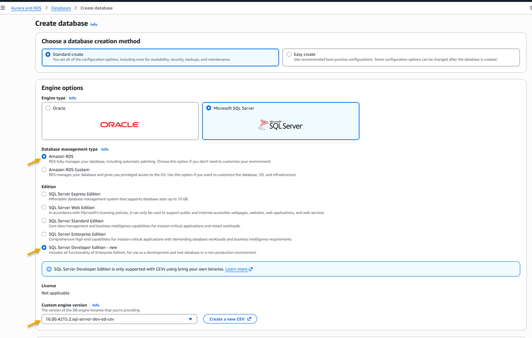
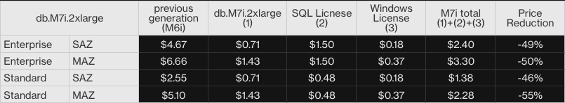
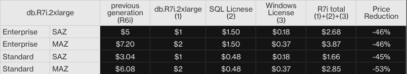
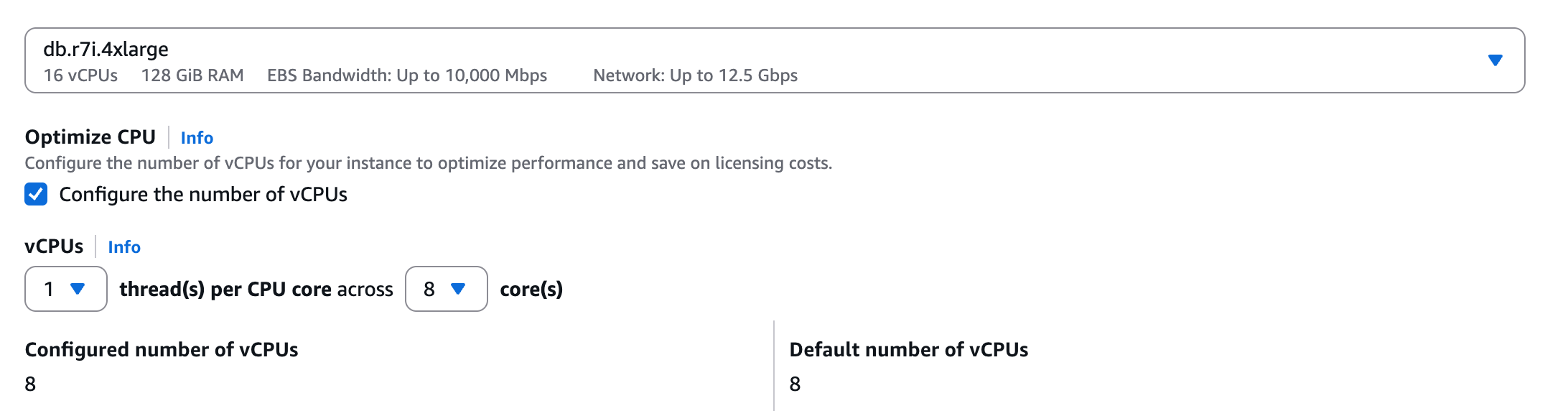
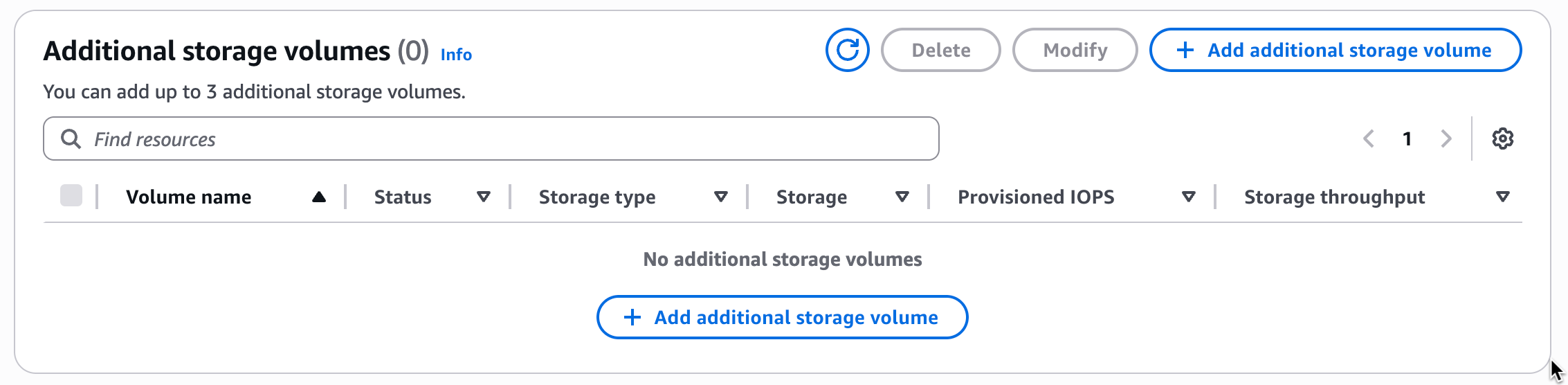
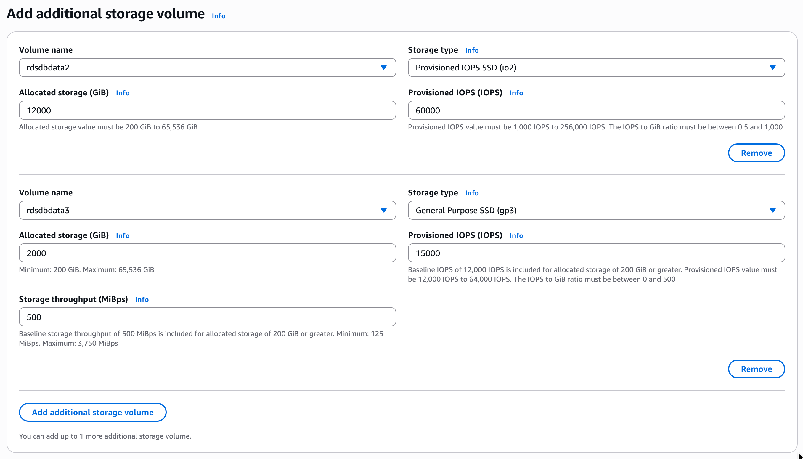
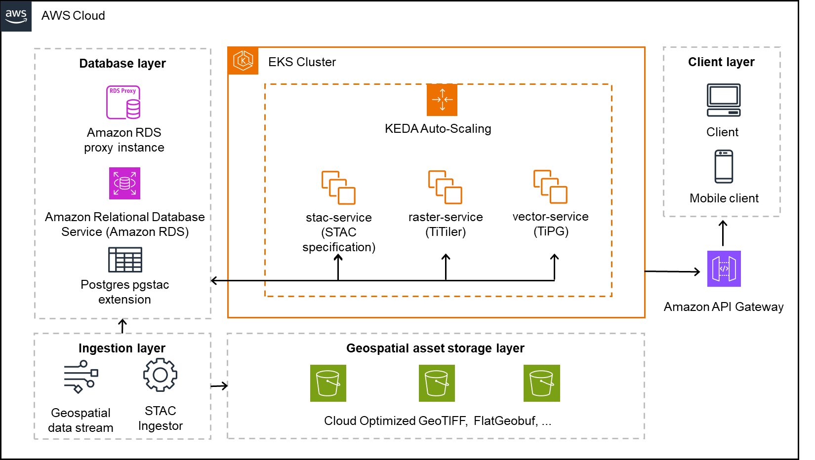
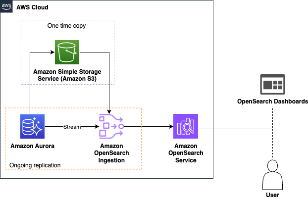
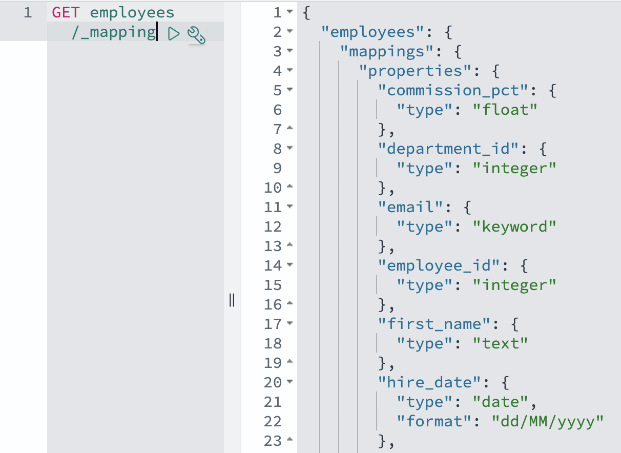
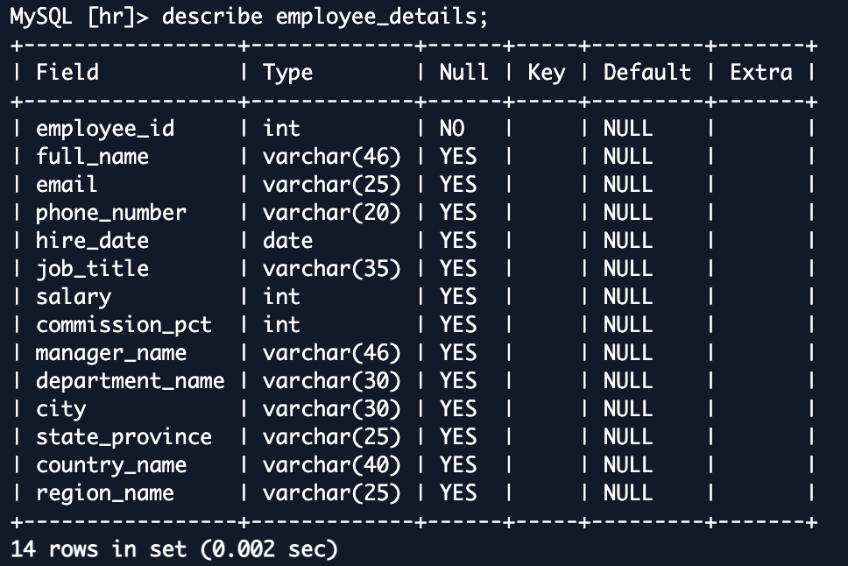
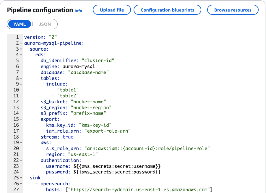
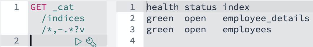
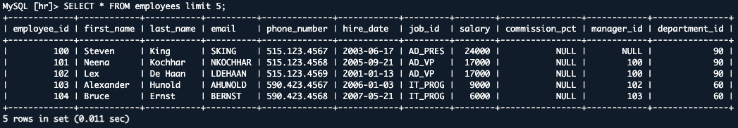

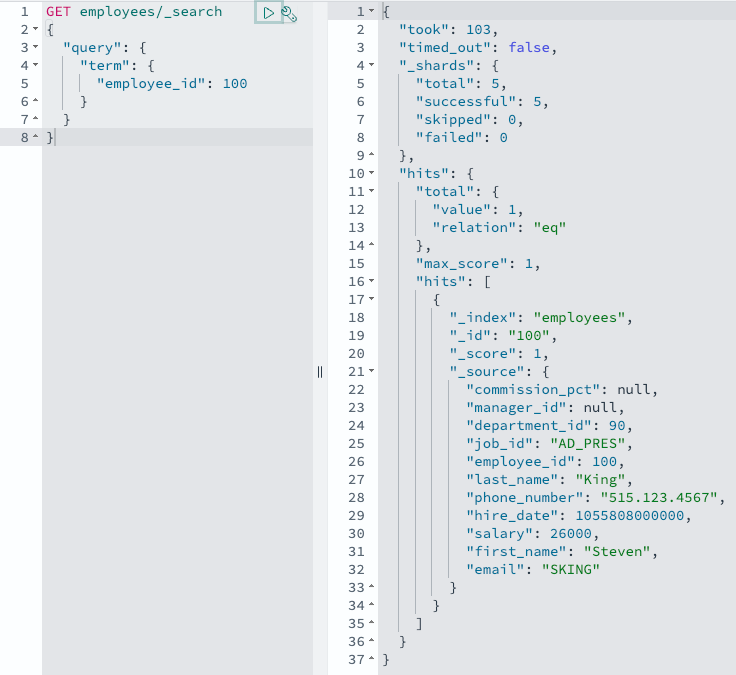
 Michael Torio is an Associate Specialist Solutions Architect at AWS focused on Amazon OpenSearch Service based out of Mountain View, CA. Michael enjoys helping customers leverage cloud technologies to solve their business challenges.
 Arjun Nambiar is a Product Manager with Amazon OpenSearch Service. He focuses on ingestion technologies that enable ingesting data from a wide variety of sources into Amazon OpenSearch Service at scale. Arjun is interested in large-scale distributed systems and cloud-centered technologies, and is based out of Seattle, Washington.


 Abhishek Pan is a Sr. Specialist SA-Data working with AWS India Public sector customers. He engages with customers to define data-driven strategy, provide deep dive sessions on analytics use cases, and design scalable and performant analytical applications. He has 12 years of experience and is passionate about databases, analytics, and AI/ML. He is an avid traveler and tries to capture the world through his lens.
 Gourang Harhare is a Senior Solutions Architect at AWS based in Pune, India. With a robust background in large-scale design and implementation of enterprise systems, application modernization, and cloud native architectures, he specializes in AI/ML, serverless, and container technologies. He enjoys solving complex problems and helping customer be successful on AWS. In his free time, he likes to play table tennis, enjoy trekking, or read books
 Kevin Phillips is a Neptune Specialist Solutions Architect working in the UK. He has 20 years of development and solutions architectural experience, which he uses to help support and guide customers. He has been enthusiastic about evangelizing graph databases since joining the Amazon Neptune team, and is happy to talk graph with anyone who will listen.
 Sandeep Varma is a principal in ZS’s Pune, India, office with over 25 years of technology consulting experience, which includes architecting and delivering innovative solutions for complex business problems leveraging AI and technology. Sandeep has been critical in driving various large-scale programs at ZS Associates. He was the founding member the Big Data Analytics Centre of Excellence in ZS and currently leads the Enterprise Service Center of Excellence. Sandeep is a thought leader and has served as chief architect of multiple large-scale enterprise big data platforms. He specializes in rapidly building high-performance teams focused on cutting-edge technologies and high-quality delivery.


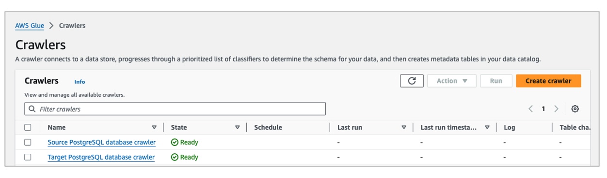


 Life is not always happy, there are difficult times. However, we can share our joys and sufferings with those we work with. The AWS Community is no exception.


 Milind Oke is a senior Redshift specialist solutions architect who has worked at Amazon Web Services for three years. He is an AWS-certified SA Associate, Security Specialty and Analytics Specialty certification holder, based out of Queens, New York.
 Aditya Samant is a relational database industry veteran with over 2 decades of experience working with commercial and open-source databases. He currently works at Amazon Web Services as a Principal Database Specialist Solutions Architect. In his role, he spends time working with customers designing scalable, secure and robust cloud native architectures. Aditya works closely with the service teams and collaborates on designing and delivery of the new features for Amazon’s managed databases.
 Happy New Year! Cloud technologies, machine learning, and generative AI have become more accessible, impacting nearly every aspect of our lives. Amazon CTO Dr. Werner Vogels offers four tech predictions for 2024 and beyond:


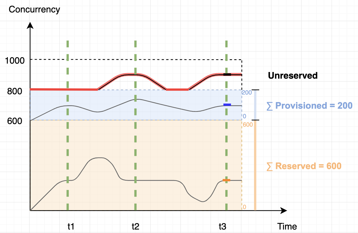


 Sriharsh Adari is a Senior Solutions Architect at Amazon Web Services (AWS), where he helps customers work backwards from business outcomes to develop innovative solutions on AWS. Over the years, he has helped multiple customers on data platform transformations across industry verticals. His core area of expertise include Technology Strategy, Data Analytics, and Data Science. In his spare time, he enjoys playing Tennis.
 Joe Morotti is a Senior Solutions Architect at Amazon Web Services (AWS), working with Enterprise customers across the Midwest US to develop innovative solutions on AWS. He has held a wide range of technical roles and enjoys showing customers the art of the possible. He has attained seven AWS certification and has a passion for AI/ML and the contact center space. In his free time, he enjoys spending quality time with his family exploring new places and overanalyzing his sports team’s performance.
 Uma Ramadoss is a specialist Solutions Architect at Amazon Web Services, focused on the Serverless platform. She is responsible for helping customers design and operate event-driven cloud-native applications and modern business workflows using services like Lambda, EventBridge, Step Functions, and Amazon MWAA.