Tag Archives: AWS ParallelCluster

Monitoring dashboard for AWS ParallelCluster

Post Syndicated from Ben Peven original https://aws.amazon.com/blogs/compute/monitoring-dashboard-for-aws-parallelcluster/

This post is contributed by Nicola Venuti, Sr. HPC Solutions Architect.

AWS ParallelCluster is an AWS-supported, open source cluster management tool that makes it easy to deploy and manage High Performance Computing (HPC) clusters on AWS. While AWS ParallelCluster includes many benefits for its users, it has not provided straightforward support for monitoring your workloads. In this post, I walk you through an add-on extension that you can use to help monitor your cloud resources with AWS ParallelCluster.

Product overview

AWS ParallelCluster offers many benefits that hide the complexity of the underlying platform and processes. Some of these benefits include:

  • Automatic resource scaling
  • A batch scheduler
  • Easy cluster management that allows you to build and rebuild your infrastructure without the need for manual actions
  • Seamless migration to the cloud supporting a wide variety of operating systems.

While all of these benefits streamline processes for you, one crucial task for HPC stakeholders that customers have found challenging with AWS ParallelCluster is monitoring.

Resources in an HPC cluster like schedulers, instances, storage, and networking are important assets to monitor, especially when you pay for what you use. Organizing and displaying all these metrics becomes challenging as the scale of the infrastructure increases or changes over time which is the typical scenario in the Cloud.

Given these challenges, AWS wants to provide AWS ParallelCluster users with two additional benefits: 1/ facilitate the optimization of price performance and 2/ visualize and monitor the components of cost for their workloads.

The HPC Solution Architects team has created an AWS ParallelCluster add-on that is easy to use and customize. In this blog post, I demonstrate how Grafana – a platform for monitoring and observability – can run on AWS ParallelCluster to enable infrastructure monitoring.

AWS ParallelCluster integrated dashboard and Grafana add-on dashboards

Many customers want a tool that consolidates information coming from different AWS services and makes it easy to monitor the computing infrastructure created and managed by AWS ParallelCluster. The AWS ParallelCluster team – just like every other service team at AWS – is open and keen to listen from our customers.

This feedback helps us inform our product roadmap and build new, customer-focused features.

We recently released AWS ParallelCluster 2.10.0 based on customer feedback. Here are some key features have been released with it:

  • Support for the CentOS 8 Operating System: Customers can now choose CentOS 8 as their base operating system of choice to run their clustersfor both x86 and Arm architectures.
  • Support for P4d instances along with NVIDIA GPUDirect Remote Direct Memory Access (RDMA).
  • FSx for Lustre enhancements (support for  FSx AutoImport and HDD-based support filesystem options)
  • And finally, a new CloudWatch Dashboards designed to help aggregating cluster information, metrics, and logging already available on CloudWatch.

The last of these features above, integrated CloudWatch Dashboards, are designed to help customers face the challenge of cluster monitoring mentioned above. In addition, the Grafana dashboards demonstrated later in this blog are a complementary add-on to this new, CloudWatch-based, dashboard. There are some key differences between the two, summarized in the table below.

The latter does not require any additional component or agent running on either the head or the compute nodes. It aggregates the metrics already pushed by AWS ParallelCluster on CloudWatch into a single dashboard. This translates into zero overhead for the cluster, but at the expense of less flexibility and expandability.

Instead, the Grafana-based dashboard offers additional flexibility and customizability and requires a few lightweight components installed on either the head or the compute nodes. Another key difference between the two monitoring dashboards is that the CloudWatch based one requires AWS credentials, IAM User and Roles configured and access to the AWS web-console, while the Grafana-based one has its-own built-in authentication and authorization system unrelated from the AWS account, end-users or HPC admins might not have permissions (or simply are not willing) to access the AWS Management Console in order to monitor their clusters.

CloudWatch based dashboard Grafana-based monitoring add-on
No additional component Grafana + Prometheus
No overhead Minimal overhead
Little to no expandability Support full customizability
Requires AWS credentials and IAM configured Custom credentials, no AWS access required
Custom user-interface

Grafana add-on dashboards on GitHub

There are many components of an HPC cluster to monitor. Moreover, the cluster is built on a system that is continuously evolving: AWS ParallelCluster and AWS services in general are updated and new features are released often. Because of this, we wanted to have a monitoring solution that is developed on flexible components, that can evolve rapidly. So, we released a Grafana add-on as an open-source project onto this GitHub repository.

Releasing it as an open-source project allows us to more easily and frequently release new updates and enhancements. It also enables users to customize and extend its functionalities by adding new dashboards, or extending the dashboards functionalities (like GPU monitoring or track EC2 Spot Instance interruptions).

At the moment, this new solution is composed of the following open-source components:

  • Grafana is an open-source platform for monitoring and observing. Grafana allows you to query, visualize, alert, and understand your metrics. It also helps you create, explore, and share dashboards fostering a data-driven culture.
  • Prometheus is an open source project for systems and service monitoring from the Cloud Native Computing Foundation. It collects metrics from configured targets at given intervals, evaluates rule expressions, displays the results, and can trigger alerts if some condition is observed to be true.
  • The Prometheus Pushgateway is an open source tool that allows ephemeral and batch jobs to expose their metrics to Prometheus.
  • NGINX is an HTTP and reverse proxy server, a mail proxy server, and a generic TCP/UDP proxy server.
  • Prometheus-Slurm-Exporter is a Prometheus collector and exporter for metrics extracted from the Slurm resource scheduling system.
  • Node_exporter is a Prometheus exporter for hardware and OS metrics exposed by *NIX kernels, written in Go with pluggable metric collectors.

Note: while almost all components are under the Apache2 license, only Prometheus-Slurm-Exporter is licensed under GPLv3. You should be aware of this license and accept its terms before proceeding and installing this component.

The dashboards

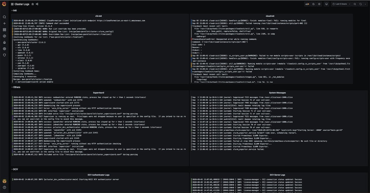
I demonstrate a few different Grafana dashboards in this post. These dashboards are available for you in the AWS Samples GitHub repository. In addition, two dashboards – still under development – are proposed in beta. The first shows the cluster logs coming from Amazon CloudWatch Logs. The second one shows the costs associated to each AWS service utilized.

All these dashboards can be used as they are or customized as you need:

  • AWS ParallelCluster Summary – This is the main dashboard that shows general monitoring info and metrics for the whole cluster. It includes: Slurm metrics, compute related metrics, storage performance metrics, and network usage.

ParallelCluster dashboard

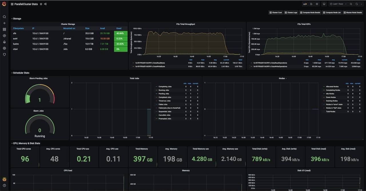
  • Master Node Details – This dashboard shows detailed metrics for the head node, including CPU, memory, network, and storage utilization.

Master node details

  • Compute Node List – This dashboard shows the list of the available compute nodes. Each entry is a link to a more detailed dashboard: the compute node details (see the following image).

Compute node list

  • Compute Node Details – Similar to the head node details, this dashboard shows detailed metrics for the compute nodes.
  • Cluster Logs – This dashboard (still under development) shows all the logs of your HPC cluster. The logs are pushed by AWS ParallelCluster to Amazon CloudWatch Logs and are reported here.

Cluster logs

  • Cluster Costs (also under development) – This dashboard shows the cost associated to AWS Service utilized by your cluster. It includes: EC2, Amazon EBS, FSx, Amazon S3, Amazon EFS. as well as an aggregation of all the costs of every single component.

Cluster costs

How to deploy it

You can simply use the post-install script that you can find in this GitHub repo as it is, or customize it as you need. For instance, you might want to change your Grafana password to something more secure and meaningful for you, or you might want to customize some dashboards by adding additional components to monitor.

#Load AWS Parallelcluster environment variables
. /etc/parallelcluster/cfnconfig
#get GitHub repo to clone and the installation script
monitoring_url=$(echo ${cfn_postinstall_args}| cut -d ',' -f 1 )
monitoring_dir_name=$(echo ${cfn_postinstall_args}| cut -d ',' -f 2 )
monitoring_tarball="${monitoring_dir_name}.tar.gz"
setup_command=$(echo ${cfn_postinstall_args}| cut -d ',' -f 3 )
monitoring_home="/home/${cfn_cluster_user}/${monitoring_dir_name}"
case ${cfn_node_type} in
    MasterServer)
        wget ${monitoring_url} -O ${monitoring_tarball}
        mkdir -p ${monitoring_home}
        tar xvf ${monitoring_tarball} -C ${monitoring_home} --strip-components 1
    ;;
    ComputeFleet)
    ;;
esac
#Execute the monitoring installation script
bash -x "${monitoring_home}/parallelcluster-setup/${setup_command}" >/tmp/monitoring-setup.log 2>&1
exit $?

The proposed post-install script takes care of installing and configuring everything for you. Although a few additional parameters are needed in the AWS ParallelCluster configuration file: the post-install argument, additional IAM policies, custom security group, and a tag. You can find an AWS ParallelCluster template here.

Please note that, at the moment, the post install script has only been tested using Amazon Linux 2.

Add the following parameters to your AWS ParallelCluster configuration file, and then build up your cluster:

base_os = alinux2
post_install = s3://<my-bucket-name>/post-install.sh
post_install_args = https://github.com/aws-samples/aws-parallelcluster-monitoring/tarball/main,aws-parallelcluster-monitoring,install-monitoring.sh
additional_iam_policies = arn:aws:iam::aws:policy/CloudWatchFullAccess,arn:aws:iam::aws:policy/AWSPriceListServiceFullAccess,arn:aws:iam::aws:policy/AmazonSSMFullAccess,arn:aws:iam::aws:policy/AWSCloudFormationReadOnlyAccess
tags = {"Grafana" : "true"}

Make sure that port 80 and port 443 of your head node are accessible from the internet or from your network. You can achieve this by creating the appropriate security group via AWS Management Console or via Command Line Interface (AWS CLI), see the following example:

aws ec2 create-security-group --group-name my-grafana-sg --description "Open Grafana dashboard ports" —vpc-id vpc-1a2b3c4d
aws ec2 authorize-security-group-ingress --group-id sg-12345 --protocol tcp --port 443 —cidr 0.0.0.0/0
aws ec2 authorize-security-group-ingress --group-id sg-12345 --protocol tcp --port 80 —cidr 0.0.0.0/0

There is more information on how to create your security groups here.

Finally, set the additional_sg parameter in the [VPC] section of your AWS ParallelCluster configuration file.

After your cluster is created, you can open a web-browser and connect to https://your_public_ip. You should see a landing page with links to the Prometheus database service and the Grafana dashboards.

Size your compute and head nodes

We looked into resource utilization of the components required for building this monitoring solution. In particular, the Prometheus node exporter installed in the compute nodes uses a small (almost negligible) number of CPU cycles, memory, and network.

Depending on the size of your cluster the components installed on the head node (see the list in the chapter “Solution components” of this blog) it might require additional CPU, memory and network capabilities. In particular, if you expect to run a large-scale cluster (hundreds of instances) because of the higher volume of network traffic due to the compute nodes continuously pushing metrics into the head node, we recommend you use an instance type bigger than what you planned.

We cannot advise you exactly how to size your head node because there are many factors that can influence resource utilization. The best recommendation we could give you is to use the Grafana dashboard itself to monitor the CPU, memory, disk, and most importantly, network utilization, and then resize your head node (or other components) accordingly.

Conclusions

This monitoring solution for AWS ParallelCluster is an add-on for your HPC Cluster on AWS and a complement to new features recently released in AWS ParallelCluster 2.10. This blog aimed to provide you with instructions and basic tooling that can be customized based on your needs and that can be adapted quickly as the underlying AWS services evolve.

We are open to hear from you, receive feedback, issues, and pull requests to extend its functionalities.

Fire Dynamics Simulation CFD workflow using AWS ParallelCluster, Elastic Fabric Adapter, Amazon FSx for Lustre and NICE DCV

Post Syndicated from Emma White original https://aws.amazon.com/blogs/compute/fire-dynamics-simulation-cfd-workflow-using-aws-parallelcluster-elastic-fabric-adapter-amazon-fsx-for-lustre-and-nice-dcv/

This post was written by By Kevin Tuil, AWS HPC consultant 

Modeling fires is key for many industries, from the design of new buildings, defining evacuation procedures for trains, planes and ships, and even the spread of wildfires. Modeling these fires is complex. It involves both the need to model the three-dimensional unsteady turbulent flow of the fire and the many potential chemical reactions. To achieve this, the fire modeling community has moved to higher-fidelity turbulence modeling approaches such as the Large Eddy Simulation, which requires both significant temporal and spatial resolution. It means that the computational cost for these simulations is typically in the order of days to weeks on a single workstation.
While there are a number of software packages, one of the most popular is the open-source code: Fire Dynamics Simulation (FDS) developed by National Institute of Standards and Technology (NIST).

In this blog, I focus on how AWS High Performance Computing (HPC) resources (e.g AWS ParallelCluster, Amazon FSx for Lustre, Elastic Fabric Adapter (EFA), and Amazon S3) allow FDS users to scale up beyond a single workstation to hundreds of cores to achieve simulation times of hours rather than days or weeks. In this blog, I outline the architecture needed, providing scripts and templates to compile FDS and run your simulation.

Service and solution overview

AWS ParallelCluster

AWS ParallelCluster is an open source cluster management tool that simplifies deploying and managing HPC clusters with Amazon FSx for Lustre, EFA, a variety of job schedulers, and the MPI library of your choice. AWS ParallelCluster simplifies cluster orchestration on AWS so that HPC environments become easy-to-use, even if you are new to the cloud. AWS released AWS ParallelCluster 2.9.1 and its user guide – which is the version I use in this blog.

These three AWS HPC resources are optimal for Fire Dynamics Simulation. Together, they provide easy deployment of HPC systems on AWS, low latency network communication for MPI workloads, and a fast, parallel file system.

Elastic Fabric Adapter

EFA is a critical service that provides low latency and high-bandwidth 100 Gbps network communication. EFA allows applications to scale at the level of on-premises HPC clusters with the on-demand elasticity and flexibility of the AWS Cloud. Computational Fluid Dynamics (CFD), among other tightly coupled applications, is an excellent candidate for the use of EFA.

Amazon FSx for Lustre

Amazon FSx for Lustre is a fully managed, high-performance file system, optimized for fast processing workloads, like HPC. Amazon FSx for Lustre allows users to access and alter data from either Amazon S3 or on-premises seamlessly and exceptionally fast. For example, you can launch and run a file system that provides sub-millisecond latency access to your data. Additionally, you can read and write data at speeds of up to hundreds of gigabytes per second of throughput, and millions of IOPS. This speed and low-latency unleash innovation at an unparalleled pace. This blog post uses the latest version of Amazon FSx for Lustre, which recently added a new API for moving data in and out of Amazon S3. This API also includes POSIX support, which allows files to mount with the same user id. Additionally, the latest version also includes a new backup feature that allows you to back up your files to an S3 bucket.

Solution and steps

The overall solution that I deploy in this blog is represented in the following diagram:

solution overview diagram

Step 1: Access to AWS Cloud9 terminal and upload data

There are two ways to start using AWS ParallelCluster. You can either install AWS CLI or turn on AWS Cloud9, which is a cloud-based integrated development environment (IDE) that includes a terminal. For simplicity, I use AWS Cloud9 to create the HPC cluster. Please refer to this link to proceed to AWS Cloud9 set up and to this link for AWS CLI setup.

Once logged into your AWS Cloud9 instance, the first thing you want to create is the S3 bucket. This bucket is key to exchange user data in and out from the corporate data center and the AWS HPC cluster. Please make sure that your bucket name is unique globally, meaning there is only one worldwide across all AWS Regions.

aws s3 mb s3://fds-smv-bucket-unique
make_bucket: fds-smv-bucket-unique

Download the latest FDS-SMV Linux version package from the official NIST website. It looks something like: FDS6.7.4_SMV6.7.14_lnx.sh

For the geometry, it should be renamed to “geometry.fds”, and must be uploaded to your AWS Cloud9 or directly to your S3 bucket.

Please note that once the FDS-SMV package has been downloaded locally to the instance, you must upload it to the S3 bucket using the following command.

aws s3 cp FDS6.7.4_SMV6.7.14_lnx.sh s3://fds-smv-bucket-unique
aws s3 cp geometry.fds s3://fds-smv-bucket-unique

You use the same S3 bucket to install FDS-SMV later on with the Amazon FSx for Lustre File System.

Step 2: Set up AWS ParallelCluster

You can install AWS ParallelCluster running the following command from your AWS Cloud9 instance:

sudo pip install aws-parallelcluster

Once it is installed, you can run the following command to check the version:

pcluster version 

At the time of writing this blog, 2.9.1 is the most up-to-date version.

Then use the text editor of your choice and open the configuration file as follows:

vim ~/.parallelcluster/config

Replace the bolded section, if not yet filled in, by your own information and save the configuration file.

[aws]
aws_region_name = <AWS-REGION>

[global]
sanity_check = true
cluster_template = fds-smv-cluster
update_check = true

[vpc public]
vpc_id = vpc-<VPC-ID>
master_subnet_id = subnet-<SUBNET-ID>

[cluster fds-smv-cluster]
key_name = <Key-Name>
vpc_settings = public
compute_instance_type=c5n.18xlarge
master_instance_type=c5.xlarge
initial_queue_size = 0
max_queue_size = 100
scheduler=slurm
cluster_type = ondemand
s3_read_write_resource=arn:aws:s3:::fds-smv-bucket-unique*
placement_group = DYNAMIC
placement = compute
base_os = alinux2
tags = {"Name" : "fds-smv"}
disable_hyperthreading = true
fsx_settings = fsxshared
enable_efa = compute
dcv_settings = hpc-dcv

[dcv hpc-dcv]
enable = master

[fsx fsxshared]
shared_dir = /fsx
storage_capacity = 1200
import_path = s3://fds-smv-bucket-unique
imported_file_chunk_size = 1024
export_path = s3://fds-smv-bucket-unique

[aliases]
ssh = ssh {CFN_USER}@{MASTER_IP} {ARGS}

Let’s review the different sections of the configuration file and explain their role:

  • scheduler: Supported job schedulers are SGE, TORQUE, SLURM and AWS Batch. I have selected SLURM for this example.
  • cluster_type: You have the choice between On-Demand (ondemand) or Spot Instances (spot) for your compute instances. For On-Demand, instances are available for use without condition (if available in the Region selected) at a certain price per hour with the pay-as-you-go model, meaning that as soon as they are started, they are reserved for your utilization. For Spot Instances, you can take advantage of unused EC2 capacity in the AWS Cloud. Spot Instances are available at up to a 90% discount compared to On-Demand Instance prices. You can use Spot Instances for various stateless, fault-tolerant, or flexible applications such as HPC, for more information about Spot Instances, feel free to visit this webpage.
  • s3_read_write_resource: This parameter allows you to read and write objects directly on your S3 bucket from the cluster you created without additional permissions. It acts as a role for your cluster, allowing you access to your specified S3 bucket.  
  • placement_groupUse DYNAMIC to ensure that your instances are located as physically close to one another as possible. Close placement minimizes the latency between compute nodes and takes advantage of EFA’s low latency networking.
  • placement: By selecting compute you only enforce compute instances to be placed within the same placement group, leaving the head node placement free.
  • compute_instance_type:Select C5n.18xlarge because it is optimized for compute-intensive workloads and supports EFA for better scaling of HPC applications. Note that EFA is supported only for specific instance types. Please visit currently supported instances for more information.
  • master_instance_type:This can be any instance type. As traffic between head and compute nodes is relatively small, and the head node runs during the entire lifetime of the cluster, I use c5.xlarge because it is inexpensive and is a good fit for this use case.
  • initial_queue_size:You start with no compute instances after the HPC cluster is up. This means that any new job submitted has some delay (time for the nodes to be powered on) before they are seen as available by the job scheduler. This helps you pay for what you use and keeps costs as low as possible.
  • max_queue_size:Limit the maximum compute fleet to 100 instances. This allows you room to scale your jobs up to a large number of cores, while putting a limit on the number of compute nodes to help control costs.
  • base_osFor this blog, select Amazon Linux 2 (alinux2) as a base OS. Currently we also support Amazon Linux (alinux), CentOS 7 (centos7), Ubuntu 16.04 (ubuntu1604), and Ubuntu 18.04 (ubuntu1804) with EFA.
  • disable_hyperthreading: This setting turns off hyperthreading (true) on your cluster, which is the right configuration in this use case.[fsx fsxshared]: This section contains the settings to define your FSx for Lustre parallel file system, including the location where the shared directory is mounted, the storage capacity for the file system, the chunk size for files to be imported, and the location from which the data will be imported. You can read more about FSx for Lustre here.
  • enable_efa: Mark as (true) in this use case since it is a tightly coupled CFD simulation use case.
  • dcv_settings:With AWS ParallelCluster, you can use NICE DCV to support your remote visualization needs.
  • [dcv hpc-dcv]:This section contains the settings to define your remote visualization setup. You can read more about DCV with AWS ParallelCluster here.
  • import_path: This parameter enables all the objects on the S3 bucket available when creating the cluster to be seen directly from the FSx for Lustre file system. In this case, you are able to access the FDS-SMV package and the geometry under the /fsx mounted folder.
  • export_path: This parameter is useful for backup purposes using the Data Repository Tasks. I share more details about this in step 7 (optional).

Step 3: Create the HPC cluster and log in

Now, you can create the HPC cluster, named fds-smv. It takes around 10 minutes to complete and you can see the status changing (going through the different AWS CloudFormation template steps). At the end of creation, two IP addresses are prompted, a public IP and/or a private IP depending on your network choice.

pcluster create fds-smv
Creating stack named: parallelcluster-fds-smv
Status: parallelcluster-fds-smv - CREATE_COMPLETE                               
MasterPublicIP: X.X.X.X
ClusterUser: ec2-user
MasterPrivateIP: X.X.X.X

In order to log in, you must use the key you specified in the AWS ParallelCluster configuration file before creating the cluster:

pcluster ssh fds-smv -i <Key-Name>

You should now be logged in as an ec2-user (since we are using Amazon Linux 2 base OS).

Step 4: Install FDS-SMV package

Now that the HPC cluster using AWS ParallelCluster is set up, it is time to install the FDS-SMV package.  In the prior steps, you uploaded both the FDS-SMV package and the geometry to your S3 bucket. Since you enabled “import_path” to that bucket, they are already available on the Amazon FSx for Lustre storage under /fsx.

Run the script as follows and select /fsx/fds-smv as final target for installation:

cd /fsx
./FDS6.7.4_SMV6.7.14_lnx.sh
[ec2-user@ip-X-X-X-X fsx]$ ./FDS6.7.4_SMV6.7.14_lnx.sh 

Installing FDS and Smokeview  for Linux

Options:
  1) Press <Enter> to begin installation [default]
  2) Type "extract" to copy the installation files to:
     FDS6.7.4_SMV6.7.14_lnx.tar.gz
 

FDS install options:
  Press 1 to install in /home/ec2-user/FDS/FDS6 [default]
  Press 2 to install in /opt/FDS/FDS6
  Press 3 to install in /usr/local/bin/FDS/FDS6
  Enter a directory path to install elsewhere
/fsx/fds-smv

It is important to source the following scripts as part of the installed packages to check if the installation is successful with the correct versions. Here is the correct output you should get:

[ec2-user@ip-X-X-X-X ~]$ source /fsx/fds-smv/bin/SMV6VARS.sh 
[ec2-user@ip-X-X-X-X ~]$ source /fsx/fds-smv/bin/FDS6VARS.sh 
[ec2-user@ip-X-X-X-X ~]$ fds -version
FDS revision       : FDS6.7.4-0-gbfaa110-release
MPI library version: Intel(R) MPI Library 2019 Update 4 for Linux* OS

[ec2-user@ip-10-0-2-233 ~]$ smokeview -version

Smokeview  SMV6.7.14-0-g568693b-release - Mar  9 2020

Revision         : SMV6.7.14-0-g568693b-release
Revision Date    : Wed Mar 4 23:13:42 2020 -0500
Compilation Date : Mar  9 2020 16:31:22
Compiler         : Intel C/C++ 19.0.4.243
Checksum(SHA1)   : e801eace7c6597dc187739e51ba6f546bfde4e48
Platform         : LINUX64

Important notes:

The way FDS-SMV package has been installed is the default installation. Binaries are already compiled and Intel MPI libraries are embedded as part of the installation package. It is what one would call a self-contained application. For further builds and source codes, please visit this webpage.

Step 5: Running the fire dynamics simulation using FDS

Now that everything is installed, it is time to create the SLURM submission script. In this step, you take advantage of the FSx for Lustre File System, the compute-optimized instance, and the EFA network to maximize simulation performance.

cd /fsx/
vi fds-smv.sbatch

Here is the information you should specify in your submission script:

#!/bin/bash
#SBATCH --job-name=fds-smv-job
#SBATCH --ntasks=<Total number of MPI processes>
#SBATCH --ntasks-per-node=36
#SBATCH --output=%x_%j.out

source /fsx/fds-smv/bin/FDS6VARS.sh
source /fsx/fds-smv/bin/SMV6VARS.sh

module load intelmpi 

export OMP_NUM_THREADS=1
export I_MPI_PIN_DOMAIN=omp

cd /fsx/<results>

time mpirun -ppn 36 -np <Total number of MPI processes>  fds geometry.fds

Replace the <results> with the one of your choice, and don’t forget to copy the geometry.fds file in it before submitting your job. Once ready, save the file and submit the job using the following command:

sbatch fds-smv.sbatch 

If you decided to build your HPC cluster with c5n.18xlarge instances, the number of MPI processes per node is 36 since you turned off the hyperthreading, and that the instance has 36 physical cores. That is the meaning of the “#SBATCH --ntasks-per-node=36” line.

For any run exceeding 36 MPI processes, the job is split among multiple instances and take advantage of EFA for internode communication.

It is important to note that FDS only allows the number of MPI processes to be equal to the number of meshes in the input geometry (geometry.fds in this scenario). In case the number of meshes in the input geometry cannot be modified, OpenMP threads can be enabled and efficiently increase performance. Do this using up to four OpenMP Threads across four CPU cores attached to one MPI process.

Please read best practices provided by NIST for that topic on their user guide.

In order to take advantage of the distributed computing capability of FDS, it is mandatory to work first on the input geometry, and divide it into the appropriate number of meshes. It is also highly advised to evenly distribute the number of cells/elements per mesh across all meshes. This best practice optimizes the load balancing for each CPU core.

Step 6: Visualizing the results using NICE DCV and SMV

In order to visualize results, you must connect to the head node using NICE DCV streaming protocol.

As a reminder, the current instance type for the head node is a c5.xlarge, which is not a graphics-accelerated instance. For heavy and GPU intensive visualization, it is important to set up a more appropriate instance such as the G4 instance group.

Go back to your AWS Cloud9 instance, open a new terminal side by side to your session connected to your AWS HPC cluster, and enter the following command in the terminal:

pcluster dcv connect fds-smv -k <Key-Name>

You are provided a one-time HTTPS URL available for a short period of time in order to connect to your head node using the NICE DCV protocol.

Once connected, open the terminal inside your session and source the FDS-SMV scripts as before:

source /fsx/fds-smv/bin/FDS6VARS.sh
source /fsx/fds-smv/bin/SMV6VARS.sh

Navigate to your <results> folder and start SMV with your result.

I have selected one of the geometries named fire_whirl_pool.fds in the Examples folder, part of the default FDS-SMV installation package located here:

/fsx/fds-smv/Examples/Fires/fire_whirl_pool.fds

You can find other scenarios under the Examples folder to run some more use cases if you did not already choose your geometry.fds file.

Now you can run SMV and visualize your results:

smokeview fire_whirl_pool.smv

SMV (smokeview) takes as an input .smv extension files, please replace with your appropriate file. If you have already chosen your geometry.fds, then run the following command:

smokeview geometry.smv

The application then open as follows, and you can visualize the results. The following image is an output of the SOOT DENSITY of the 3D smoke.

fire simulation picture

Step 7 (optional): Back up your FDS-SMV results to an S3 bucket

First update the AWS CLI to its most recent version. It is compatible with 1.16.309 and above.

After running your FDS-SMV simulation, you can back up your data in /fsx to the S3 bucket you used earlier to upload the installation package, and input files using Data Repository Tasks.

Data Repository Tasks represent bulk operations between your Amazon FSx for Lustre file system and your S3 bucket. One of the jobs is to export your changed file system contents back to its linked S3 bucket.

Open your AWS Cloud9 terminal and exit the HPC head node cluster. Retrieve your Amazon FSx for Lustre ID using:

aws fsx describe-file-systems

It looks something like, fs-0533eebf1148fc8dd. Then create a backup of the data as follows:

aws fsx create-data-repository-task --file-system-id fs-0533eebf1148fc8dd --type EXPORT_TO_REPOSITORY --paths results --report Enabled=true,Scope=FAILED_FILES_ONLY,Format=REPORT_CSV_20191124,Path=s3://fds-smv-bucket-unique/

The following are definitions about the command parameters:

  • file-system-id: Your file system ID.
  • type EXPORT_TO_REPOSITORY: Exports the data back to the S3 bucket.
  • paths results: The directory you want to export to your S3 bucket. If you have more than one folder to back up, use a comma-separated notation such as: results1,results2,…
  • Format=REPORT_CSV_20191124: Note this is only the name the Amazon FSx Lustre supports. Please keep it the same.

You can check the backup status by running:

aws fsx describe-data-repository-tasks

Please wait for the copy to be achieved, once finished you should see on the Lifecycle line "Lifecycle": "SUCCEEDED"

Also go back to your S3 bucket, and your folder(s) should appear with all the files correctly uploaded from your /fsx folder you specified.

In terms of data management, Amazon S3 is an important service. You started by uploading installation package and geometry files from an external source, such as your laptop or an on-premises system. Then made these files available to the AWS HPC cluster under the Amazon FSx for Lustre file system and ran the simulation. Finally, you backed up the results from the Amazon FSx for Lustre to Amazon S3. You can also decide to download the results on Amazon S3 back to your local system if needed.

Step 8: Delete your AWS resources created during the deployment of this blog

After your run is completed and your data backed up successfully (Step 7 is optional) on your S3 bucket, you can then delete your cluster by using the following command in your Cloud9 terminal:

pcluster delete fds-smv

Warning:

If you run the command above all resources you created during this blog are automatically deleted beside your Cloud9 session and your data on your S3 bucket you created earlier.

Your S3 bucket still contains your input “geometry.fds” and your installation package “FDS6.7.4_SMV6.7.14_lnx.sh” files.

If you selected to back up your data during Step 7 (optional), then your S3 bucket also contains that data on top of the two previous files mentioned above.

If you want to delete your S3 bucket and all data mentioned above, go to your AWS Management Console, select S3 service then select your S3 bucket and hit delete on the top section.

If you want to terminate your Cloud9 session, go to your AWS Management Console, select Cloud9 service then select your session and hit delete on the top right section.

After performing these operations, there will be no more resources running on AWS related to this blog.

Conclusion

I showed that AWS ParallelCluster, Amazon FSx for Lustre, EFA, and Amazon S3 are key AWS services and features for HPC workloads such as CFD and in particular for FDS.

You can achieve simulation times of hours on AWS rather than days or weeks on a single workstation.

Please visit this workshop  for a more in-depth tutorial on running Fire Dynamics Simulation on AWS and our HPC dedicated homepage.