All posts by Emma White

Insulating AWS Outposts Workloads from Amazon EC2 Instance Size, Family, and Generation Dependencies

Post Syndicated from Emma White original https://aws.amazon.com/blogs/compute/insulating-aws-outposts-workloads-from-amazon-ec2-instance-size-family-and-generation-dependencies/

This post is written by Garry Galinsky, Senior Solutions Architect.

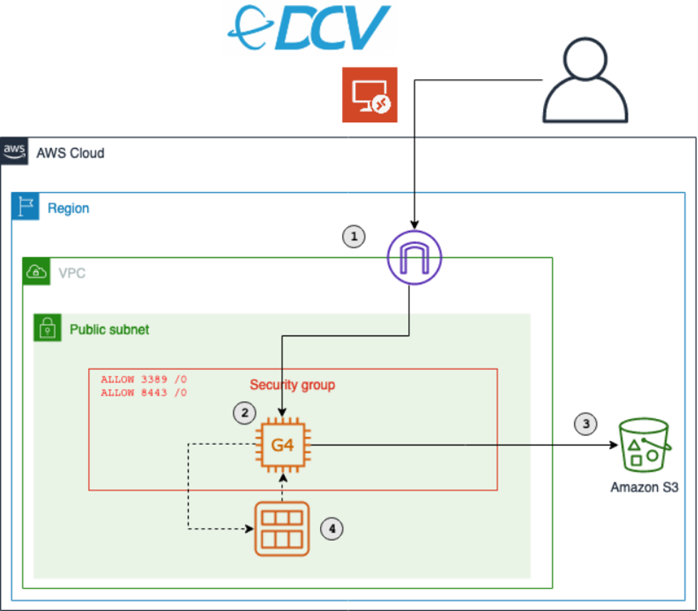
AWS Outposts is a fully managed service that offers the same AWS infrastructure, AWS services, APIs, and tools to virtually any datacenter, co-location space, or on-premises facility for a truly consistent hybrid experience. AWS Outposts is ideal for workloads that require low-latency access to on-premises systems, local data processing, data residency, and application migration with local system interdependencies.

Unlike AWS Regions, which offer near-infinite scale, Outposts are limited by their provisioned capacity, EC2 family and generations, configured instance sizes, and availability of compute capacity that is not already consumed by other workloads. This post explains how Amazon EC2 Fleet can be used to insulate workloads running on Outposts from EC2 instance size, family, and generation dependencies, reducing the likelihood of encountering an error when launching new workloads or scaling existing ones.

Product Overview

Outposts is available as a 42U rack that can scale to create pools of on-premises compute and storage capacity. When you order an Outposts rack, you specify the quantity, family, and generation of Amazon EC2 instances to be provisioned. As of this writing, five EC2 families, each of a single generation, are available on Outposts (m5, c5, r5, g4dn, and i3en). However, in the future, more families and generations may be available, and a given Outposts rack may include a mix of families and generations. EC2 servers on Outposts are partitioned into instances of homogenous or heterogeneous sizes (e.g., large, 2xlarge, 12xlarge) based on your workload requirements.

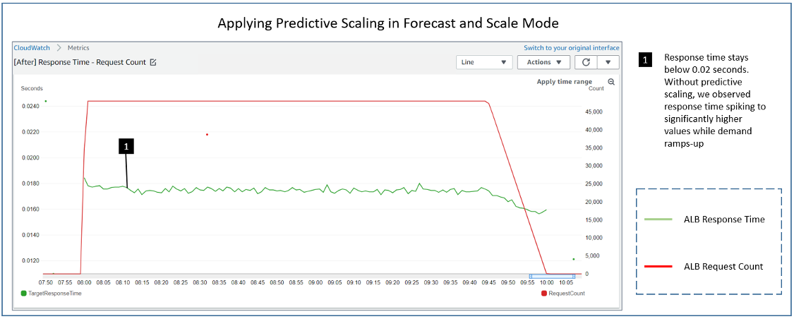
Workloads deployed through AWS CloudFormation or scaled through Amazon EC2 Auto Scaling generally assume that the required EC2 instance type will be available when the deployment or scaling event occurs. Although in the Region this is a reasonable assumption, the same is not true for Outposts. Whether as a result of competing workloads consuming the capacity, the Outpost having been configured with limited capacity for a given instance size, or an Outpost update resulting in instances being replaced with a newer generation, a deployment or scaling event tied to a specific instance size, family, and generation may encounter an InsufficentInstanceCapacity error (ICE). And this may occur even though sufficient unused capacity of a different size, family, or generation is available.

EC2 Fleet

Amazon EC2 Fleet simplifies the provisioning of Amazon EC2 capacity across different Amazon EC2 instance types and Availability Zones, as well as across On-Demand, Amazon EC2 Reserved Instances (RI), and Amazon EC2 Spot purchase models. A single API call lets you provision capacity across EC2 instance types and purchase models in order to achieve the desired scale, performance, and cost.

An EC2 Fleet contains a configuration to launch a fleet, or group, of EC2 instances. The LaunchTemplateConfigs parameter lets multiple instance size, family, and generation combinations be specified in a priority order.

This feature is commonly used in AWS Regions to optimize fleet costs and allocations across multiple deployment strategies (reserved, on-demand, and spot), while on Outposts it can be used to eliminate the tight coupling of a workload to specific EC2 instances by specifying multiple instance families, generations, and sizes.

Launch Template Overrides

The EC2 Fleet LaunchTemplateConfigs definition describes the EC2 instances required for the fleet. A specific parameter of this definition, the Overrides, can include prioritized and/or weighted options of EC2 instances that can be launched to satisfy the workload. Let’s investigate how you can use Overrides to decouple the EC2 size, family, and generation dependencies.

Overriding EC2 Instance Size

Let’s assume our Outpost was provisioned with an m5 server. The server is the equivalent of an m5.24xlarge, which can be configured into multiple instances. For example, the server can be homogeneously provisioned into 12 x m5.2xlarge, or heterogeneously into 1 x m5.8xlarge, 3 x m5.2xlarge, 8 x m5.xlarge, and 4 x m5.large. Let’s assume the heterogeneous configuration has been applied.

Our workload requires compute capacity equivalent to an m5.4xlarge (16 vCPUs, 64 GiB memory), but that instance size is not available on the Outpost. Attempting to launch this instance would result in an InsufficentInstanceCapacity error. Instead, the following LaunchTemplateConfigs override could be used:

"Overrides": [
    {
        "InstanceType": "m5.4xlarge",
        "WeightedCapacity": 1.0,
        "Priority": 1.0
    },
    {
        "InstanceType": "m5.2xlarge",
        "WeightedCapacity": 0.5,
        "Priority": 2.0
    },
    {
        "InstanceType": "m5.8xlarge",
        "WeightedCapacity": 2.0,
        "Priority": 3.0
    }
]

The Priority describes our order of preference. Ideally, we launch a single m5.4xlarge instance, but that’s not an option. Therefore, in this case, the EC2 Fleet would move to the next priority option, an m5.2xlarge. Given that an m5.2xlarge (8 vCPUs, 32 GiB memory) offers only half of the resource of the m5.4xlarge, the override includes the WeightedCapacity parameter of 0.5, resulting in two m5.2xlarge instances launching instead of one.

Our overrides include a third, over-provisioned and less preferable option, should the Outpost lack two m5.2xlarge capacity: launch one m5.8xlarge. Operating within finite resources requires tradeoffs, and priority lets us optimize them. Note that had the launch required 2 x m5.4xlarge, only one instance of m5.8xlarge would have been launched.

Overriding EC2 Instance Family

Let’s assume our Outpost was provisioned with an m5 and a c5 server, homogeneously partitioned into 12 x m5.2xlarge and 12 x c5.2xlarge instances. Our workload requires compute capacity equivalent to a c5.2xlarge instance (8 vCPUs, 16 GiB memory). As our workload scales, more instances must be launched to meet demand. If we couple our workload to c5.2xlarge, then our scaling will be blocked as soon as all 12 instances are consumed. Instead, we use the following LaunchTemplateConfigs override:

"Overrides": [
    {
        "InstanceType": "c5.2xlarge",
        "WeightedCapacity": 1.0,
        "Priority": 1.0
    },
    {
        "InstanceType": "m5.2xlarge",
        "WeightedCapacity": 1.0,
        "Priority": 2.0
    }
]

The Priority describes our order of preference. Ideally, we scale more c5.2xlarge instances, but when those are not an option EC2 Fleet would launch the next priority option, an m5.2xlarge. Here again the outcome may result in over-provisioned memory capacity (32 vs 16 GiB memory), but it’s a reasonable tradeoff in a finite resource environment.

Overriding EC2 Instance Generation

Let’s assume our Outpost was provisioned two years ago with an m5 server. Since then, m6 servers have become available, and there’s an expectation that m7 servers will be available soon. Our single-generation Outpost may unexpectedly become multi-generation if the Outpost is expanded, or if a hardware failure results in a newer generation replacement.

Coupling our workload to a specific generation could result in future scaling challenges. Instead, we use the following LaunchTemplateConfigs override:

"Overrides": [
    {
        "InstanceType": "m6.2xlarge",
        "WeightedCapacity": 1.0,
        "Priority": 1.0
    },
    {
        "InstanceType": "m5.2xlarge",
        "WeightedCapacity": 1.0,
        "Priority": 2.0
    },
    {
        "InstanceType": "m7.2xlarge",
        "WeightedCapacity": 1.0,
        "Priority": 3.0
    }

]

Note the Priority here, our preference is for the current generation m6, even though it’s not yet provisioned in our Outpost. The m5 is what would be launched now, given that it’s the only provisioned generation. However, we’ve also future-proofed our workload by including the yet unreleased m7.

Deploying an EC2 Fleet

To deploy an EC2 Fleet, you must:

  1. Create a launch template, which streamlines and standardizes EC2 instance provisioning by simplifying permission policies and enforcing best practices across your organization.
  2. Create a fleet configuration, where you set the number of instances required and specify the prioritized instance family/generation combinations.
  3. Launch your fleet (or a single EC2 instance).

These steps can be codified through AWS CloudFormation or executed through AWS Command Line Interface (CLI) commands. However, fleet definitions cannot be implemented by using the AWS Console. This example will use CLI commands to conduct these steps.

Prerequisites

To follow along with this tutorial, you should have the following prerequisites:

Create a Launch Template

Launch templates let you store launch parameters so that you do not have to specify them every time you launch an EC2 instance. A launch template can contain the Amazon Machine Images (AMI) ID, instance type, and network settings that you typically use to launch instances. For more details about launch templates, reference Launch an instance from a launch template .

For this example, we will focus on these specifications:

  • AMI image ImageId
  • Subnet (the SubnetId associated with your Outpost)
  • Availability zone (the AvailabilityZone associated with your Outpost)
  • Tags

Create a launch template configuration (launch-template.json) with the following content:

{
    "ImageId": "<YOUR-AMI>",
    "NetworkInterfaces": [
        {
            "DeviceIndex": 0,
            "SubnetId": "<YOUR-OUTPOST-SUBNET>"
        }
    ],
    "Placement": {
        "AvailabilityZone": "<YOUR-OUTPOST-AZ>"
    },
    "TagSpecifications": [
        {
            "ResourceType": "instance",
            "Tags": [
                {
                    "Key": "<YOUR-TAG-KEY>",
                    "Value": "<YOUR-TAG-VALUE>"
                }
            ]
        }
    ]
}

Create your launch template using the following CLI command:

aws ec2 create-launch-template \
  --launch-template-name <YOUR-LAUNCH-TEMPLATE-NAME> \
  --launch-template-data file://launch-template.json

You should see a response like this:

{
    "LaunchTemplate": {
        "LaunchTemplateId": "lt-010654c96462292e8",
        "LaunchTemplateName": "<YOUR-LAUNCH-TEMPLATE-NAME>",
        "CreateTime": "2021-07-12T15:55:00+00:00",
        "CreatedBy": "arn:aws:sts::<YOUR-AWS-ACCOUNT>:assumed-role/<YOUR-AWS-ROLE>",
        "DefaultVersionNumber": 1,
        "LatestVersionNumber": 1
    }
}

The value for LaunchTemplateId is the identifier for your newly created launch template. You will need this value lt-010654c96462292e8 in the subsequent step.

Create a Fleet Configuration

Refer to Generate an EC2 Fleet JSON configuration file for full documentation on the EC2 Fleet configuration.

For this example, we will use this configuration to override a mix of instance size, family, and generation. The override includes three EC2 instance types:

  • m5.large, the instance family and generation currently available on the Outpost.
  • m6.large, a forthcoming family and generation not yet available for Outposts.
  • m7.large, a potential future family and generation.

Create an EC2 fleet configuration (ec2-fleet.json) with the following content (note that the LaunchTemplateId was the value returned in the prior step):

{
    "TargetCapacitySpecification": {
        "TotalTargetCapacity": 1,
        "OnDemandTargetCapacity": 1,
        "SpotTargetCapacity": 0,
        "DefaultTargetCapacityType": "on-demand"
    },
    "OnDemandOptions": {
        "AllocationStrategy": "prioritized",
        "SingleInstanceType": true,
        "SingleAvailabilityZone": true,
        "MinTargetCapacity": 1
    },
    "LaunchTemplateConfigs": [
        {
            "LaunchTemplateSpecification": {
                "LaunchTemplateId": "lt-010654c96462292e8",
                "Version": "1"
            },
            "Overrides": [
                {
                    "InstanceType": "m6.2xlarge",
                    "WeightedCapacity": 1.0,
                    "Priority": 1.0
                },
                {
                    "InstanceType": "c5.2xlarge",
                    "WeightedCapacity": 1.0,
                    "Priority": 2.0
                },
                {
                    "InstanceType": "m5.large",
                    "WeightedCapacity": 0.25,
                    "Priority": 3.0
                },
                {
                    "InstanceType": "m5.2xlarge",
                    "WeightedCapacity": 1.0,
                    "Priority": 4.0
                },
                {
                    "InstanceType": "r5.2xlarge",
                    "WeightedCapacity": 1.0,
                    "Priority": 5.0
                }


            ]
        }
    ],
    "Type": "instant"
}

Launch the Single Instance Fleet

To launch the fleet, execute the following CLI command (this will launch a single instance, but a similar process can be used to launch multiple):

aws ec2 create-fleet \
  --cli-input-json file://ec2-fleet.json

You should see a response like this:

{
    "FleetId": "fleet-dc630649-5d77-60b3-2c30-09808ef8aa90",
    "Errors": [
        {
            "LaunchTemplateAndOverrides": {
                "LaunchTemplateSpecification": {
                    "LaunchTemplateId": "lt-010654c96462292e8",
                    "Version": "1"
                },
                "Overrides": {
                    "InstanceType": "m6.2xlarge",
                    "WeightedCapacity": 1.0,
                    "Priority": 1.0
                }
            },
            "Lifecycle": "on-demand",
            "ErrorCode": "InvalidParameterValue",
            "ErrorMessage": "The instance type 'm6.2xlarge' is not supported in Outpost 'arn:aws:outposts:us-west-2:111111111111:outpost/op-0000ffff0000fffff'."
        },
        {
            "LaunchTemplateAndOverrides": {
                "LaunchTemplateSpecification": {
                    "LaunchTemplateId": "lt-010654c96462292e8",
                    "Version": "1"
                },
                "Overrides": {
                    "InstanceType": "c5.2xlarge",
                    "WeightedCapacity": 1.0,
                    "Priority": 2.0
                }
            },
            "Lifecycle": "on-demand",
            "ErrorCode": "InsufficientCapacityOnOutpost",
            "ErrorMessage": "There is not enough capacity on the Outpost to launch or start the instance."
        }
    ],
    "Instances": [
        {
            "LaunchTemplateAndOverrides": {
                "LaunchTemplateSpecification": {
                    "LaunchTemplateId": "lt-010654c96462292e8",
                    "Version": "1"
                },
                "Overrides": {
                    "InstanceType": "m5.large",
                    "WeightedCapacity": 0.25,
                    "Priority": 3.0
                }
            },
            "Lifecycle": "on-demand",
            "InstanceIds": [
                "i-03d6323c8a1df8008",
                "i-0f62593c8d228dba5",
                "i-0ae25baae1f621c15",
                "i-0af7e688d0460a60a"
            ],
            "InstanceType": "m5.large"
        }
    ]
}

Results

Navigate to the EC2 Console where you will find new instances running on your Outpost. An example is shown in the following screenshot:

EC2 running instances, AWS console, network view, filtered by tag

Although multiple instance size, family, and generation combinations were included in the Overrides, only the c5.large was available on the Outpost. Instead of launching one m6.2xlarge, four c5.large were launched in order to compensate for their lower WeightedCapacity. From the fleet-create response, the overrides were clearly evaluated in priority order with the error messages explaining why the top two overrides were ignored.

Clean up

AWS CLI EC2 commands can be used to create fleets but can also be used to delete them.

To clean up the resources created in this tutorial:

    1. Note the FleetId values returned in the create-fleet command.
    2. Run the following command for each fleet created:
aws ec2 delete-fleets \
  --fleet-ids  \
  --terminate-instances
  1. Note the launch-template-name used in the create-launch-template command.
  2. Run the following command for each fleet created:
{
    "SuccessfulFleetDeletions": [
        {
            "CurrentFleetState": "deleted_terminating",
            "PreviousFleetState": "active",
            "FleetId": "fleet-dc630649-5d77-60b3-2c30-09808ef8aa90"
        }
    ],
    "UnsuccessfulFleetDeletions": []
}
  1. Clean up any resources you created for the prerequisites.

Conclusion

This post discussed how EC2 Fleet can be used to decouple the availability of specific EC2 instance sizes, families, and generation from the ability to launch or scale workloads. On an Outpost provisioned with multiple families of EC2 instances (say m5 and c5) and different sizes (say m5.large and m5.2xlarge), EC2 Fleet can be used to satisfy a workload launch request even if the capacity of the preferred instance size, family, or generation is unavailable.

To learn more about AWS Outposts, check out the Outposts product page. To see a full list of pre-defined Outposts configurations, visit the Outposts pricing page

Monitoring delay of AWS Batch jobs in transit before execution

Post Syndicated from Emma White original https://aws.amazon.com/blogs/compute/monitoring-delay-of-aws-batch-jobs-in-transit-before-execution/

This post is written by Nikhil Anand, Solutions Architect 

AWS Batch enables developers, scientists, and engineers to easily and efficiently run hundreds of thousands of batch processing jobs on AWS. With AWS Batch you no longer have to install and manage batch computing software or server clusters used to run your jobs. This lets you focus on analyzing results and solving problems, not managing infrastructure. When you use AWS Batch, in the job lifetime, a job goes through several states. When creating a compute environment to run the Batch jobs and submit Batch jobs, a settings misconfiguration could cause the job to get stuck in a transit state. This means the job will not proceed to the desired RUNNING state – a common issue faced by most customers.

If your compute environment contains compute resources, but your jobs don’t progress beyond the RUNNABLE state, then something is preventing the jobs from being placed on a compute resource. There are various reasons why a job could remain in the RUNNABLE state. The usual call to action is referring the troubleshooting documentation in order to fix the issue. Similarly, if your job is dependent on another job, then the job would stay in the PENDING state.

However, if you have scheduled actions to be completed with Batch jobs, or if you do not have any mechanism monitoring the jobs, then your jobs might stay in any of the transit states if left unattended. You may end up continuing forward, unaware that your job has yet to run. Eventually, when you see the jobs not progressing beyond the RUNNABLE or PENDING state, you miss the task that the job was expected to do in the given timeframe. This can result in additional time and effort troubleshooting the stuck job.

To prevent this accidental avoidance or lack of in-transit job monitoring, this post provides a monitoring solution for jobs in transit (from the SUBMITTED to the RUNNING state) in AWS Batch.

You can configure a threshold monitoring duration for your jobs so that if a job stays in SUBMITTED/PENDING/RUNNABLE longer than that, then you get a notification. For example, you might have a job that you would want to proceed to the RUNNING state in approximately 15 minutes since the job submission. Sometimes a slight misconfiguration can cause the job to get stuck in RUNNABLE indefinitely. In that case, you can set a threshold of 15 minutes. Or, suppose you have a job that is dependent on the other job that is stuck in processing. In these situations, once the specified duration is crossed, you are notified about your job staying in transit beyond your defined threshold status.

The solution is deployed by using AWS CloudFormation.

Overview of solution

The solution creates an Amazon CloudWatch Events rule that triggers an AWS Lambda function on a schedule. Then, the Lambda function checks every job in transit for more than ‘X’ seconds on all compute environments since the job submission. Specify your own value for ‘X’ when you launch the AWS CloudFormation stack. The solution consists of the following components created via CloudFormation:

  • An Amazon CloudWatch event rule to monitor the submitted jobs in Batch using the target Lambda function
  • An AWS Lambda function with the logic to monitor the submitted jobs and trigger Amazon Simple Notification Service (Amazon SNS) notifications
  • A Lambda execution AWS Identity and Access Management (IAM) role
  • An Amazon SNS topic to be subscribed by end users in order to be notified about the submitted jobs

The solution components and workflow.

Prerequisites

For this walkthrough, you should have the following prerequisites:

Walkthrough

To provision the necessary solution components, use this CloudFormation template. 

  1. While launching the CloudFormation stack, you will be asked to input the following information in addition to the CloudFormation stack name:
    1. The upper threshold (in seconds) for the jobs to stay in the transit state
    2. The evaluation period after which the Lambda runs periodically
    3. The email ID to get notifications after the job stays in the transit state for the defined threshold value.

pecify parameter values during CloudFormation stack launch

  1. Once the stack is created, the following resources will be provisioned – SNS topic, CloudWatch Events rule, Lambda function, Lambda invoke permissions, and Lambda execution role. View it in the ‘Resources’ tab of your CloudFormation stack.

Successful creation of the CloudFormation stack

  1. After the stack is created, the email ID you entered in step III above will receive an email from Amazon SNS in order to confirm the Amazon SNS subscription.

Subscription confirmation email that you receive on the specified email ID.

Click Confirm subscription in the email.

Subscription confirmed.

  1. Based on the customer’s inputs during stack launch, a Lambda function will be periodically invoked to look out for Batch jobs stuck in the RUNNABLE state for the defined threshold.
  2. An Amazon SNS notification is sent out at the evaluation periods with the job IDs of the jobs that have stayed stuck in the RUNNABLE state.

Verifying the solution

Launch your monitoring solution by using the CloudFormation template. Once the stack creation is complete, I get an email to subscribe to the SNS topic. Then, I subscribe to the SNS topic.

Click to launch Stack. 

Submit a job in AWS Batch by using console, CLI, or SDK. To test the solution, submit a job, Job1, to a job queue associated with a compute environment with no public subnets. Compute resources require access in order to communicate with the Amazon ECS service endpoint. This can be done through an interface VPC endpoint or your compute resources having public IP addresses. Since the compute environment was configured to only have a private subnet, Job1 will not proceed from the RUNNABLE state. Similarly, submit another job, Job2, and during submission add a dependency of Job1 on Job2. Therefore, Job2 will not proceed from the PENDING state. Thus, creating a sample space wherein two jobs will be stuck in transit.

AWS Batch jobs submitted and in transit.

Based on the CloudFormation template inputs, you will get notified on the subscribed Email ID when the job stays in transit for more than ‘X’ seconds (the input provided during stack launch).

otification received for the jobs that stayed in transit longer than expected.

Modifications

The Lambda function uses the ListJobs API call. The maximum number of results is returned by ListJobs in paginated output. Therefore, if you are submitting many jobs, then you must modify the Lambda function to fetch more results from the initial response of the call by using the nextToken response element. Use this nextToken element and iterate through in a loop to keep fetching the paginated results until there are no further nextToken elements present.

Cleaning up

To avoid incurring future charges, delete the resources. You can delete the CloudFormation stack that will clean up every resource that it provisioned for the monitoring solution.

Conclusion

This solution lets you detect AWS Batch jobs that remain in the transit state longer than expected. It provides you with an efficient way to monitor your Batch jobs. If the jobs stay in the RUNNABLE/PENDING/SUBMITTED state for a significant amount of time, then it is indicative of potential misconfiguration with either the compute environment setup, or with the job parameters that were passed during the job submission. An early notification around the issue can help you troubleshoot the misconfigurations early on and take subsequent actions.

If you have multiple jobs that remain in the RUNNABLE state and you realize that they will not proceed further to the RUNNING state due to a misconfiguration, then you can shut down all RUNNABLE jobs by using a simple bash script.

For additional references regarding troubleshooting RUNNABLE jobs in AWS Batch, refer to the suggested Knowledge Center article and the troubleshooting documentation.

Optimizing Apache Flink on Amazon EKS using Amazon EC2 Spot Instances

Post Syndicated from Emma White original https://aws.amazon.com/blogs/compute/optimizing-apache-flink-on-amazon-eks-using-amazon-ec2-spot-instances/

This post is written by Kinnar Sen, Senior EC2 Spot Specialist Solutions Architect

Apache Flink is a distributed data processing engine for stateful computations for both batch and stream data sources. Flink supports event time semantics for out-of-order events, exactly-once semantics, backpressure control, and optimized APIs. Flink has connectors for third-party data sources and AWS Services, such as Apache Kafka, Apache NiFi, Amazon Kinesis, and Amazon MSK. Flink can be used for Event Driven (Fraud Detection), Data Analytics (Ad-Hoc Analysis), and Data Pipeline (Continuous ETL) applications. Amazon Elastic Kubernetes Service (Amazon EKS) is the chosen deployment option for many AWS customers for Big Data frameworks such as Apache Spark and Apache Flink. Flink has native integration with Kubernetes allowing direct deployment and dynamic resource allocation.

In this post, I illustrate the deployment of scalable, highly available (HA), resilient, and cost optimized Flink application using Kubernetes via Amazon EKS and Amazon EC2 Spot Instances (Spot). Learn how to save money on big data streaming workloads by implementing this solution.

Overview

Amazon EC2 Spot Instances

Amazon EC2 Spot Instances let you take advantage of spare EC2 capacity in the AWS Cloud and are available at up to a 90% discount compared to On-Demand Instances. Spot Instances receive a two-minute warning when these instances are about to be reclaimed by Amazon EC2. There are many graceful ways to handle the interruption. Recently EC2 Instance rebalance recommendation has been added to send proactive notifications when a Spot Instance is at elevated risk of interruption. Spot Instances are a great way to scale up and increase throughput of Big Data workloads and has been adopted by many customers.

Apache Flink and Kubernetes

Apache Flink is an adaptable framework and it allows multiple deployment options and one of them being Kubernetes. Flink framework has a couple of key building blocks.

  • Job Client submits the job in form of a JobGraph to the Job Manager.
  • Job Manager plays the role of central work coordinator which distributes the job to the Task Managers.
  • Task Managers are the worker component, which runs the operators for source, transformations and sinks.
  • External components which are optional such as Resource Provider, HA Service Provider, Application Data Source, Sinks etc., and this varies with the deployment mode and options.

Image shows Flink application deployment architecture with Job Manager, Task Manager, Scheduler, Data Flow Graph, and client.

Flink supports different deployment (Resource Provider) modes when running on Kubernetes. In this blog we will use the Standalone Deployment mode, as we just want to showcase the functionality. We recommend first-time users however to deploy Flink on Kubernetes using the Native Kubernetes Deployment.

Flink can be run in different modes such as Session, Application, and Per-Job. The modes differ in cluster lifecycle, resource isolation and execution of the main() method. Flink can run jobs on Kubernetes via Application and Session Modes only.

  • Application Mode: This is a lightweight and scalable way to submit an application on Flink and is the preferred way to launch application as it supports better resource isolation. Resource isolation is achieved by running a cluster per job. Once the application shuts down all the Flink components are cleaned up.
  • Session Mode: This is a long running Kubernetes deployment of Flink. Multiple applications can be launched on a cluster and the applications competes for the resources. There may be multiple jobs running on a TaskManager in parallel. Its main advantage is that it saves time on spinning up a new Flink cluster for new jobs, however if one of the Task Managers fails it may impact all the jobs running on that.

Amazon EKS

Amazon EKS is a fully managed Kubernetes service. EKS supports creating and managing Spot Instances using Amazon EKS managed node groups following Spot best practices. This enables you to take advantage of the steep savings and scale that Spot Instances provide for interruptible workloads. EKS-managed node groups require less operational effort compared to using self-managed nodes. You can learn more in the blog “Amazon EKS now supports provisioning and managing EC2 Spot Instances in managed node groups.”

Apache Flink and Spot

Big Data frameworks like Spark and Flink are distributed to manage and process high volumes of data. Designed for failure, they can run on machines with different configurations, inherently resilient and flexible. Spot Instances can optimize runtimes by increasing throughput, while spending the same (or less). Flink can tolerate interruptions using restart and failover strategies.

Fault Tolerance

Fault tolerance is implemented in Flink with the help of check-pointing the state. Checkpoints allow Flink to recover state and positions in the streams. There are two per-requisites for check-pointing a persistent data source (Apache Kafka, Amazon Kinesis) which has the ability to replay data and a persistent distributed storage to store state (Amazon Simple Storage Service (Amazon S3), HDFS).

Cost Optimization

Job Manager and Task Manager are key building blocks of Flink. The Task Manager is the compute intensive part and Job Manager is the orchestrator. We would be running Task Manager on Spot Instances and Job Manager on On Demand Instances.

Scaling

Flink supports elastic scaling via Reactive Mode, Task Managers can be added/removed based on metrics monitored by an external service monitor like Horizontal Pod Autoscaling (HPA). When scaling up new pods would be added, if the cluster has resources they would be scheduled it not then they will go in pending state. Cluster Autoscaler (CA) detects pods in pending state and new nodes will be added by EC2 Auto Scaling. This is ideal with Spot Instances as it implements elastic scaling with higher throughput in a cost optimized way.

Tutorial: Running Flink applications in a cost optimized way

In this tutorial, I review steps, which help you launch cost optimized and resilient Flink workloads running on EKS via Application mode. The streaming application will read dummy Stock ticker prices send to an Amazon Kinesis Data Stream by Amazon Kinesis Data Generator, try to determine the highest price within a per-defined window, and output will be written onto Amazon S3 files.

Image shows Flink application pipeline with data flowing from Amazon Kinesis Data Generator to Kinesis Data Stream, processed in Apache Flink and output being written in Amazon S3

The configuration files can be found in this github location. To run the workload on Kubernetes, make sure you have eksctl and kubectl command line utilities installed on your computer or on an AWS Cloud9 environment. You can run this by using an AWS IAM user or role that has the Administrator Access policy attached to it, or check the minimum required permissions for using eksctl. The Spot node groups in the Amazon EKS cluster can be launched both in a managed or a self-managed way, in this post I use the EKS Managed node group for Spot Instances.

Steps

When we deploy Flink in Application Mode it runs as a single application. The cluster is exclusive for the job. We will be bundling the user code in the Flink image for that purpose and upload in Amazon Elastic Container Registry (Amazon ECR). Amazon ECR is a fully managed container registry that makes it easy to store, manage, share, and deploy your container images and artifacts anywhere.

1. Build the Amazon ECR Image

  • Login using the following cmd and don’t forget to replace the AWS_REGION and AWS_ACCOUNT_ID with your details.

aws ecr get-login-password --region ${AWS_REGION} | docker login --username AWS —password-stdin ${ACCOUNT_ID}.dkr.ecr.${AWS_REGION}.amazonaws.com

  • Create a repository

aws ecr create-repository --repository-name flink-demo --image-scanning-configuration scanOnPush=true —region ${AWS_REGION}

  • Build the Docker image:

Download the Docker file. I am using multistage docker build here. The sample code is from Github’s Amazon Kinesis Data Analytics Java examples. I modified the code to allow checkpointing and change the sliding window interval. Build and push the docker image using the following instructions.

docker build --tag flink-demo .

  • Tag and Push your image to Amazon ECR

docker tag flink-demo:latest ${ACCOUNT_ID}.dkr.ecr.${AWS_REGION}.amazonaws.com/flink-demo:latest
docker push ${ACCOUNT_ID}.dkr.ecr.${AWS_REGION}.
amazonaws.com/flink-demo:latest

2. Create Amazon S3/Amazon Kinesis Access Policy

First, I must create an access policy to allow the Flink application to read/write from Amazon fFS3 and read Kinesis data streams. Download the Amazon S3 policy file from here and modify the <<output folder>> to an Amazon S3 bucket which you have to create.

  • Run the following to create the policy. Note the ARN.

aws iam create-policy --policy-name flink-demo-policy --policy-document file://flink-demo-policy.json

3. Cluster and node groups deployment

  • Create an EKS cluster using the following command:

eksctl create cluster –name= flink-demo --node-private-networking --without-nodegroup --asg-access –region=<<AWS Region>>

The cluster takes approximately 15 minutes to launch.

  • Create the node group using the nodeGroup config file. I am using multiple nodeGroups of different sizes to adapt Spot best practice of diversification.  Replace the <<Policy ARN>> string using the ARN string from the previous step.

eksctl create nodegroup -f managedNodeGroups.yml

  • Download the Cluster Autoscaler and edit it to add the cluster-name (flink-demo)

curl -LO https://raw.githubusercontent.com/kubernetes/autoscaler/master/cluster-autoscaler/cloudprovider/aws/examples/cluster-autoscaler-autodiscover.yaml

4. Install the Cluster AutoScaler using the following command:

kubectl apply -f cluster-autoscaler-autodiscover.yaml

  • Using EKS Managed node groups requires significantly less operational effort compared to using self-managed node group and enables:
    • Auto enforcement of Spot best practices.
    • Spot Instance lifecycle management.
    • Auto labeling of Pods.
  • eksctl has integrated amazon-ec2-instance-selector to enable auto selection of instances based on the criteria passed. This has multiple benefits
    • ‘instance diversification’ is implemented by enabling multiple instance types selection in the node group which works well with CA
    • Reduces manual effort of selecting the instances.
  • We can create node group manifests using ‘dryrun’ and then create node groups using that.

eksctl create cluster --name flink-demo --instance-selector-vcpus=2 --instance-selector-memory=4 --dry-run

eksctl create node group -f managedNodeGroups.yml

5. Create service accounts for Flink

$ kubectl create serviceaccount flink-service-account
$ kubectl create clusterrolebinding flink-role-binding-flink --clusterrole=edit --serviceaccount=default:flink-service-account

6. Deploy Flink

This install folder here has all the YAML files required to deploy a standalone Flink cluster. Run the install.sh file. This will deploy the cluster with a JobManager, a pool of TaskManagers and a Service exposing JobManager’s ports.

  • This is a High-Availability(HA) deployment of Flink with the use of Kubernetes high availability service.
  • The JobManager runs on OnDemand and TaskManager on Spot. As the cluster is launched in Application Mode, if a node is interrupted only one job will be restarted.
  • Autoscaling is enabled by the use of ‘Reactive Mode’. Horizontal Pod Autoscaler is used to monitor the CPU load and scale accordingly.
  • Check-pointing is enabled which allows Flink to save state and be fault tolerant.

Image shows the Flink dashboard highlighting checkpoints for a job

7. Create Amazon Kinesis data stream and send dummy data      

Log in to AWS Management Console and create a Kinesis data stream name ‘ExampleInputStream’. Kinesis Data Generator is used to send data to the data stream. The template of the dummy data can be found here. Once this sends data the Flink application starts processing.

Image shows Amazon Kinesis Data Generator console sending data to Kinesis Data Strea

Observations

Spot Interruptions

If there is an interruption then the Flick application will be restarted using check-pointed data. The JobManager will restore the job as highlighted in the following log. The node will be replaced automatically by the Managed Node Group.

mage shows logs from a Flink job highlighting job restart using checkpoints.

One will be able to observe the graceful restart in the Flink UI.

Image shows the Flink dashboard highlighting job restart after failure.

AutoScaling

You can observe the elastic scaling using logs. The number of TaskManagers in the Flink UI will also reflect the scaling state.

Image shows kubectl output showing status of HPA during scale-out

Cleanup

If you are trying out the tutorial, run the following steps to make sure that you don’t encounter unwanted costs.

  • Run the delete.sh file.
  • Delete the EKS cluster and the node groups:
    • eksctl delete cluster --name flink-demo
  • Delete the Amazon S3 Access Policy:
    • aws iam delete-policy --policy-arn <<POLICY ARN>>
  • Delete the Amazon S3 Bucket:
    • aws s3 rb --force s3://<<S3_BUCKET>>
  • Delete the CloudFormation stack related to Kinesis Data Generator named ‘Kinesis-Data-Generator-Cognito-User’
  • Delete the Kinesis Data Stream.

Conclusion

In this blog, I demonstrated how you can run Flink workloads on a Kubernetes Cluster using Spot Instances, achieving scalability, resilience, and cost optimization. To cost optimize your Flink based big data workloads you should start thinking about using Amazon EKS and Spot Instances.

Use Amazon EC2 for cost-efficient cloud gaming with pay-as-you-go pricing

Post Syndicated from Emma White original https://aws.amazon.com/blogs/compute/use-amazon-ec2-for-cost-efficient-cloud-gaming-with-pay-as-you-go-pricing/

This post is written by Markus Ziller, Solutions Architect

Since AWS launched in 2006, cloud computing disrupted traditional IT operations by providing a more cost-efficient, scalable, and secure alternative to owning hardware and data centers. Similarly, cloud gaming today enables gamers to play video games with pay-as-you go pricing. This removes the need of high upfront investments in gaming hardware. Cloud gaming platforms like Amazon Luna are an entryway, but customers are limited to the games available on the service. Furthermore, many customers also prefer to own their games, or they already have a sizable collection. For those use cases, vendor-neutral software like NICE DCV or Parsec are powerful solutions for streaming your games from anywhere.

This post shows a way to stream video games from the AWS Cloud to your local machine. I will demonstrate how you can provision a powerful gaming machine with pay-as-you-go pricing that allows you to play even the most demanding video games with zero upfront investment into gaming hardware.

The post comes with code examples on GitHub that let you follow along and replicate this post in your account.

In this example, I use the AWS Cloud Development Kit (AWS CDK), an open source software development framework, to model and provision cloud application resources. Using the CDK can reduce the complexity and amount of code needed to automate resource deployment.

Overview of the solution

The main services in this solution are Amazon Elastic Compute Cloud (Amazon EC2) and Amazon Elastic Block Store (Amazon EBS). The architecture is as follows:

The architecture of the solution. It shows an EC2 instance of the G4 family deployed in a public subnet. The EC2 instances communicates with S3. Also shown is how a security group controls access from users to the EC2 instance

The key components of this solution are described in the following list. During this post, I will explain each component in detail. Deploy this architecture with the sample CDK project that comes with this blog post.

  1. An Amazon Virtual Private Cloud (Amazon VPC) that lets you launch AWS resources in a logically isolated virtual network. This includes a network configuration that lets you connect with instances in your VPC on ports 3389 and 8443.
  2. An Amazon EC2 instance of the G4 instance family. Amazon EC2 G4 instances are the most cost-effective and versatile GPU instances. Utilize G4 instances to run your games.
  3. Access to an Amazon Simple Storage Service (Amazon S3) bucket. S3 is an object storage that contains the graphics drivers required for GPU instances.
  4. A way to create a personal gaming Amazon Machine Images (AMI). AMIs mean that you only need to conduct the initial configuration of your gaming instance once. After that, create new gaming instances on demand from your AMI.

Walkthrough

The following sections walk through the steps required to set up your personal gaming AMI. You will only have to do this once.

For this walkthrough, you need:

  • An AWS account
  • Installed and authenticated AWS CLI
  • Installed Node.js, TypeScript
  • Installed git
  • Installed AWS CDK

You will also need an EC2 key pair for the initial instance setup. List your available key pairs with the following CLI command:

aws ec2 describe-key-pairs --query 'KeyPairs[*].KeyName' --output table

Alternatively, create a new key pair with the CLI. You will need the created .pem file later, so make sure to keep it.

KEY_NAME=Gaming
aws ec2 create-key-pair --key-name $KEY_NAME –query 'KeyMaterial' --output text > $KEY_NAME.pem

Checkout and deploy the sample stack

  1. After completing the prerequisites, clone the associated GitHub repository by running the following command in a local directory:git clone [email protected]:aws-samples/cloud-gaming-on-ec2-instances
  1. Open the repository in your preferred local editor, and then review the contents of the *.ts files in cdk/bin/ and cdk/lib/
  1. In gaming-on-g4-instances.ts you will find two CDK stacks: G4DNStack and G4ADStack. A CDK stack is a unit of deployment. All AWS resources defined within the scope of a stack, either directly or indirectly, are provisioned as a single unit.

The architecture for both stacks is similar, and it only differs in the instance type that will be deployed.

G4DNStack and G4ADStack share parameters that determine the configuration of the EC2 instance, the VPC network and the preinstalled software. The stacks come with defaults for some parameters – I recommend keeping the default values.

EC2

  • instanceSize: Sets the EC2 size. Defaults to g4dn.xlarge and g4ad.4xlarge, respectively. Check the service page for a list of valid configurations.
  • sshKeyName: The name of the EC2 key pair you will use to connect to the instance. Ensure you have access to the respective .pem file.
  • volumeSizeGiB: The root EBS volume size. Around 20 GB will be used for the Windows installation, the rest will be available for your software.

VPC

  • openPorts: Access from these ports will be allowed. Per default, this will allow access for Remote Desktop Protocol (RDP) (3389) and NICE DCV (8443).
  • associateElasticIp: Controls if an Elastic IP address will be created and added to the EC2 instance. An Elastic IP address is a static public IPv4 address. Contrary to dynamic IPv4 addresses managed by AWS, it will not change after an instance restart. This is an optional convenience that comes at a small cost for reserving the IP address for you.
  • allowInboundCidr: Access from this CIDR range will be allowed. This limits the IP space from where your instance is routable. It can be used to add an additional security layer. Per default, traffic from any IP address will be allowed to reach your instance. Notwithstanding allowInboundCidr, an RDP or NICE DCV connection to your instance requires valid credentials and will be rejected otherwise.

Software

For g4dn instances, one more parameter is required (see process of installing NVIDIA drivers):

  • gridSwCertUrl: The NVIDIA driver requires a certificate file, which can be downloaded from Amazon S3.

Choose an instance type based on your performance and cost requirements, and then adapt the config accordingly. I recommend starting with the G4DNStack, as it comes at the lowest hourly instance cost. If you need more graphics performance, then choose the G4ADStack for up to 40% improvement in graphics performance.

After choosing an instance, follow the instructions in the README.md in order to deploy the stack.

The CDK will create a new Amazon VPC with a public subnet. It will also configure security groups to allow inbound traffic from the CIDR range and ports specific in the config. By default, this will allow inbound traffic from any IP address. I recommend restricting access to your current IP address by going to checkip.amazonaws.com and replacing 0.0.0.0/0 with <YOUR_IP>/32 for the allowInboundCidr config parameter.

Besides the security groups, the CDK also manages all required IAM permissions.

It creates the following resources in your VPC:

  • An EC2 GPU instance running Windows Server 2019. Depending on the stack you chose, the default instance type will be g4dn.xlarge or g4ad.4xlarge. You can override this in the template. When the EC2 instance is launched, the CDK runs an instance-specific PowerShell script. This PowerShell script downloads all drivers and NICE DCV. Check the code to see the full script or add your own commands.
  • An EBS gp3 volume with your defined size (default: 150 GB).
  • An EC2 launch template.
  • (Optionally) An Elastic IP address as a static public IP address for your gaming instances.

After the stack has been deployed, you will see the following output:

The output of a CDK deployment of the CloudGamingOnG4DN stack. Shows values for Credentials, InstanceId, KeyName, LaunchTemplateId, PublicIp. Values for Credentials, InstanceId and PublicIp are redacted

Click the first link, and download the remote desktop file in order to connect to your instance. Use the .pem file from the previous step to receive the instance password.

Install drivers on EC2

You will use the RDP to initially connect to your instance. RDP provides a user with a graphical interface to connect to another computer over a network connection. RDP clients are available for a large number of platforms. Use the public IP address provided by the CDK output, the username Administrator, and the password displayed by the EC2 dialogue.

Ensure that you note the password for later steps.

Most configuration process steps are automated by the CDK. However, a few actions (e.g., driver installation) cannot be properly automated. For those, the following manual steps are required once.

Navigate to $home\Desktop\InstallationFiles. If the folder contains an empty file named “OK”, then everything was downloaded correctly and you can proceed with the installation. If you connect while the setup process is still in progress, then wait until the OK file gets created before proceeding. This typically takes 2-3 minutes.

The next step differs slightly for g4ad and g4dn instances.

g4ad instances with AMD Radeon Pro V520

Follow the instructions in the EC2 documentation to install the AMD driver from the InstallationFiles folder. The installation may take a few minutes, and it will display the following output when successfully finished.

The output of the PowerShell command that installs the graphics driver for AMD Radeon Pro V520

The contents of the InstallationFiles folder. It contains a folder 1_AMD_driver and files 2_NICEDCV-Server, 3_NICEDCV-DisplayDriver, OK

Next, install NICE DCV Server and Display driver by double-clicking the respective files. Finally, restart the instance by running the Restart-Computer PowerShell command.


g4dn instances with NVIDIA T4

Navigate to 1_NVIDIA_drivers, run the NVIDIA driver installer for Windows Server 2019 and follow the instructions.

The contents of the InstallationFiles folder. It contains a folder 1_NVIDIA_drivers and files 2_NICEDCV-Server, 3_NICEDCV-DisplayDriver, 4_update_registry, OK

Next, double-click the respective files in the InstallationFiles folder in order to install NICE DCV Server and Display driver.

Finally, right-click on 4_update_registry.ps1, and select “Run with PowerShell” to activate the driver. In order to complete the setup, restart the instance.

Install your software

After the instance restart, you can connect from your local machine to your EC2 instance with NICE DCV. The NICE DCV bandwidth-adaptive streaming protocol allows near real-time responsiveness for your applications without compromising the image accuracy. This is the recommended way to stream latency sensitive applications.

Download the NICE DCV viewer client and connect to your EC2 instance with the same credentials that you used for the RDP connection earlier. After testing the NICE DCV connection, I recommend disabling RDP by removing the corresponding rule in your security group.

You are now all set to install your games and tools on the EC2 instance. Make sure to install it on the C: drive, as you will create an AMI with the contents of C: later.

Start and stop your instance on demand

At this point, you have fully set up the EC2 instance for cloud gaming on AWS. You can now start and stop the instance when needed. The following CLI commands are all you need to remember:

aws ec2 start-instances --instance-ids <INSTANCE_ID>

aws ec2 stop-instances --instance-ids <INSTANCE_ID>

This will use the regular On-Demand instance capacity of EC2, and you will be billed hourly charges for the time that your instance is running. If your instance is stopped, you will only be charged for the EBS volume and the Elastic IP address if you chose to use one.

Launch instances from AMI

Make sure you have installed all of the applications you require on your EC2, and then create your personal gaming AMI by running the following AWS CLI command.

aws ec2 create-image --instance-id <YOUR_INSTANCE_ID> --name <THE_NAME_OF_YOUR_AMI>

Use the following command to get details about your AMI creation. When the status changes from pending to available, then your AMI is ready.

aws ec2 describe-images --owners self --query 'Images[*].[Name, ImageId, BlockDeviceMappings[0].Ebs.SnapshotId, State]' --output table

The CDK created an EC2 launch template when it deployed the stack. Run the following CLI command to spin up an EC2 instance from this template.

aws ec2 run-instances --image-id <YOUR_AMI_ID> --launch-template LaunchTemplateName=<LAUNCH_TEMPLATE_NAME> --query "Instances[*].[InstanceId, PublicIpAddress]" --output table

This command will start a new EC2 instance with the exact same configuration as your initial EC2, but with all your software already installed.

Conclusion

This post walked you through creating your personal cloud gaming stack. You are now all set to lean back and enjoy the benefits of per second billing while playing your favorite video games in the AWS cloud.

Visit the Amazon EC2 G4 instances service page to learn more about how AWS continues to push the boundaries of cost-effectiveness for graphic-intensive applications.

Building Modern Applications with Amazon EKS on Amazon Outposts

Post Syndicated from Emma White original https://aws.amazon.com/blogs/compute/building-modern-applications-with-amazon-eks-on-amazon-outposts/

This post is written by Brad Kirby, Principal Outposts Specialist, and Chris Lunsford, Senior Outposts SA. 

Customers are modernizing applications by deconstructing monolithic architectures and migrating application components into container–based, service-oriented, and microservices architectures. Modern applications improve scalability, reliability, and development efficiency by allowing services to be owned by smaller, more focused teams.

This post shows how you can combine Amazon Elastic Kubernetes Service (Amazon EKS) with AWS Outposts to deploy managed Kubernetes application environments on-premises alongside your existing data and applications.

For a brief introduction to the subject matter, the watch this video, which demonstrates:

  • The benefits of application modernization
  • How containers are an ideal enabling technology for microservices architectures
  • How AWS Outposts combined with Amazon container services enables you to unwind complex service interdependencies and modernize on-premises applications with low latency, local data processing, and data residency requirements

Understanding the Amazon EKS on AWS Outposts architecture

Amazon EKS

Many organizations chose Kubernetes as their container orchestration platform because of its openness, flexibility, and a growing pool of Kubernetes literate IT professionals. Amazon EKS enables you to run Kubernetes clusters on AWS without needing to install and manage the Kubernetes control plane. The control plane, including the API servers, scheduler, and cluster store services, runs within a managed environment in the AWS Region. Kubernetes clients (like kubectl) and cluster worker nodes communicate with the managed control plane via public and private EKS service endpoints.

AWS Outposts

The AWS Outposts service delivers AWS infrastructure and services to on-premises locations from the AWS Global Cloud Infrastructure. An Outpost functions as an extension of the Availability Zone (AZ) where it is anchored. AWS operates, monitors, and manages AWS Outposts infrastructure as part of its parent Region. Each Outpost connects back to its anchor AZ via a Service Link connection (a set of encrypted VPN tunnels). AWS Outposts extend Virtual Private Cloud (VPC) environments from the Region to on-premises locations and enables you to deploy VPC subnets to Outposts in your data center and co-location spaces. The Outposts Local Gateway (LGW) routes traffic between Outpost VPC subnets and the on-premises network.

Amazon EKS on AWS Outposts

You deploy Amazon EKS worker nodes to Outposts using self-managed node groups. The worker nodes run on Outposts and register with the Kubernetes control plane in the AWS Region. The worker nodes, and containers running on the nodes, can communicate with AWS services and resources running on the Outpost and in the region (via the Service Link) and with on-premises networks (via the Local Gateway).


You use the same AWS and Kubernetes tools and APIs to work with EKS on Outposts nodes that you use to work with EKS nodes in the Region. You can use eksctl, the AWS Management Console, AWS CLI, or infrastructure as code (IaC) tools like AWS CloudFormation or HashiCorp Terraform to create self-managed node groups on AWS Outposts.

Amazon EKS self-managed node groups on AWS Outposts

Like many customers, you might use managed node groups when you deploy EKS worker nodes in your Region, and you may be wondering, “what are self-managed node groups?”

Self-managed node groups, like managed node groups, use standard Amazon Elastic Compute Cloud (Amazon EC2) instances in EC2 Auto Scaling groups to deploy, scale-up, and scale-down EKS worker nodes using Amazon EKS optimized Amazon Machine Images (AMIs). Amazon configures the EKS optimized AMIs to work with the EKS service. The images include Docker, kubelet, and the AWS IAM Authenticator. The AMIs also contain a specialized bootstrap script /etc/eks/bootstrap.sh that allows worker nodes to discover and connect to your cluster control plane and add Kubernetes labels that identify the nodes in the cluster.

What makes the node groups self-managed? Managed node groups have additional features that simplify updating nodes in the node group. With self-managed nodes, you must implement a process to update or replace your node group when you want to update the nodes to use a new Amazon EKS optimized AMI.

You create self-managed node groups on AWS Outposts using the same process and resources that you use to deploy EC2 instances using EC2 Auto Scaling groups. All instances in a self-managed node group must:

  • Be the same Instance type
  • Be running the same Amazon Machine Image (AMI)
  • Use the same Amazon EKS node IAM role
  • Be tagged with the io/cluster/<cluster-name>=owned tag

Additionally, to deploy on AWS Outposts, instances must:

  • Use encrypted EBS volumes
  • Launch in Outposts subnets

Kubernetes authenticates all API requests to a cluster. You must configure an EKS cluster to allow nodes from a self-managed node group to join the cluster. Self-managed nodes use the node IAM role to authenticate with an EKS cluster. Amazon EKS clusters use the AWS IAM Authenticator for Kubernetes to authenticate requests and Kubernetes native Role Based Access Control (RBAC) to authorize requests. To enable self-managed nodes to register with a cluster, configure the AWS IAM Authenticator to recognize the node IAM role and assign the role to the system:bootstrappers and system:nodes RBAC groups.

In the following tutorial, we take you through the steps required to deploy EKS worker nodes on an Outpost and register those nodes with an Amazon EKS cluster running in the Region. We created a sample Terraform module aws-eks-self-managed-node-group to help you get started quickly. If you are interested, you can dive into the module sample code to see the detailed configurations for self-managed node groups.

Deploying Amazon EKS on AWS Outposts (Terraform)

To deploy Amazon EKS nodes on an AWS Outposts deployment, you must complete two high-level steps:

Step 1: Create a self-managed node group

Step 2: Configure Kubernetes to allow the nodes to register

We use Terraform in this tutorial to provide visibility (through the sample code) into the details of the configurations required to deploy self-managed node groups on AWS Outposts.

Prerequisites

To follow along with this tutorial, you should have the following prerequisites:

  • An AWS account.
  • An operational AWS Outposts deployment (Outpost) associated with your AWS account.
  • AWS Command Line Interface (CLI) version 1.25 or later installed and configured on your workstation.
  • HashiCorp Terraform version 14.6 or later installed on your workstation.
  • Familiarity with Terraform HashiCorp Configuration Language (HCL) syntax and experience using Terraform to deploy AWS resources.
  • An existing VPC that meets the requirements for an Amazon EKS cluster. For more information, see Cluster VPC considerations. You can use the Getting started with Amazon EKS guide to walk you through creating a VPC that meets the requirements.
  • An existing Amazon EKS cluster. You can use the Creating an Amazon EKS cluster guide to walk you through creating the cluster.
  • Tip: We recommend creating and using a new VPC and Amazon EKS cluster to complete this tutorial. Procedures like modifying the aws-auth ConfigMap on the cluster may impact other nodes, users, and workloads on the cluster. Using a new VPC and Amazon EKS cluster will help minimize the risk of impacting other applications as you complete the tutorial.
  • Note: Do not reference subnets deployed on AWS Outposts when creating Amazon EKS clusters in the Region. The Amazon EKS cluster control plane runs in the Region and attaches to VPC subnets in the Region availability zones.
  • A symmetric KMS key to encrypt the EBS volumes of the EKS worker nodes. You can use the alias/aws/ebs AWS managed key for this prerequisite.

Using the sample code

The source code for the amazon-eks-self-managed-node-group Terraform module is available in AWS-Samples on GitHub.

Setup

To follow along with this tutorial, complete the following steps to setup your workstation:

  1. Open your terminal.
  2. Make a new directory to hold your EKS on Outposts Terraform configurations.
  3. Change to the new directory.
  4. Create a new file named providers.tf with the following contents:
    terraform {
      required_providers {
        aws = {
          source  = "hashicorp/aws"
          version = "~> 3.27"
        }
    
        kubernetes = {
          source  = "hashicorp/kubernetes"
          version = "~> 1.13.3"
        }
      }
    }

  5. Keep your terminal open and do all the work in this tutorial from this directory.

Step 1: Create a self-managed node group

To create a self-managed node group on your Outpost

  1. Create a new Terraform configuration file named self-managed-node-group.tf.
  2. Configure the aws Terraform provider with your AWS CLI profile and Outpost parent Region:
    provider "aws" {
      region  = "us-west-2"
      profile = "default"
    }
    

  3. Configure the aws-eks-self-managed-node-group module with the following (minimum) arguments:
    • eks_cluster_name the name of your EKS cluster
    • instance_type an instance type supported on your AWS Outposts deployment
    • desired_capacity, min_size, and max_size as desired to control the number of nodes in your node group (ensure that your Outpost has sufficient resources available to run the desired number nodes of the specified instance type)
    • subnets the subnet IDs of the Outpost subnets where you want the nodes deployed
    • (Optional) Kubernetes node_labels to apply to the nodes
    • Allow ebs_encrypted and configure the ebs_kms_key_arn with KMS key you want to use to encrypt the nodes’ EBS volumes (required for Outposts deployments)

Example:

module "eks_self_managed_node_group" {
  source = "github.com/aws-samples/amazon-eks-self-managed-node-group"

  eks_cluster_name = "cmluns-eks-cluster"
  instance_type    = "m5.2xlarge"
  desired_capacity = 1
  min_size         = 1
  max_size         = 1
  subnets          = ["subnet-0afb721a5cc5bd01f"]

  node_labels = {
    "node.kubernetes.io/outpost"    = "op-0d4579457ff2dc345"
    "node.kubernetes.io/node-group" = "node-group-a"
  }

  ebs_encrypted   = true
  ebs_kms_key_arn = "arn:aws:kms:us-west-2:799838960553:key/0e8f15cc-d3fc-4da4-ae03-5fadf45cc0fb"
}

You may configure other optional arguments as appropriate for your use case – see the module README for details.

Step 2: Configure Kubernetes to allow the nodes to register

Use the following procedures to configure Terraform to manage the AWS IAM Authenticator (aws-auth) ConfigMap on the cluster. This adds the node-group IAM role to the IAM authenticator and Kubernetes RBAC groups.

Configure the Terraform Kubernetes Provider to allow Terraform to interact with the Kubernetes control plane.

Note: If you add a node group to a cluster with existing node groups, mapped IAM roles, or mapped IAM users, the aws-auth ConfigMap may already be configured on your cluster. If the ConfigMap exists, you must download, edit, and replace the ConfigMap on the cluster using kubectl. We do not provide a procedure for this operation as it may affect workloads running on your cluster. Please see the section Managing users or IAM roles for your cluster in the Amazon EKS User Guide for more information.

To check if your cluster has the aws-auth ConfigMap configured

  1. Run the aws eks --region <region> update-kubeconfig --name <cluster-name> command to update your workstation’s ~/.kube/config with the information needed to connect to your cluster, substituting your <region> and <cluster-name>.
❯ aws eks --region us-west-2 update-kubeconfig --name cmluns-eks-cluster
Updated context arn:aws:eks:us-west-2:799838960553:cluster/cmluns-eks-cluster in ~/.kube/config
  1. Run the kubectl describe configmap -n kube-system aws-auth
  • If you receive an error stating, Error from server (NotFound): configmaps "aws-auth" not found, then proceed with the following procedures to use Terraform to apply the ConfigMap.
❯ kubectl describe configmap -n kube-system aws-auth
Error from server (NotFound): configmaps "aws-auth" not found
  • If you do not receive the preceding error, and kubectl returns an aws-auth ConfigMap, then you should not use Terraform to manage the ConfigMap.

To configure the Terraform Kubernetes provider

  1. Create a new Terraform configuration file named aws-auth-config-map.tf.
  2. Add the aws_eks_cluster Terraform data source, and configure it to look up your cluster by name.
data "aws_eks_cluster" "selected" {
  name = "cmluns-eks-cluster"
}
  1. Add the aws_eks_cluster_auth Terraform data source, and configure it to look up your cluster by name.
data "aws_eks_cluster_auth" "selected" {
  name = "cmluns-eks-cluster"
}
  1. Configure the kubernetes provider with your cluster host (endpoint address), cluster_ca_certificate, and the token from the aws_eks_cluster and aws_eks_cluster_auth data sources.
provider "kubernetes" {
  load_config_file       = false
  host                   = data.aws_eks_cluster.selected.endpoint
  cluster_ca_certificate = base64decode(data.aws_eks_cluster.selected.certificate_authority[0].data)
  token                  = data.aws_eks_cluster_auth.selected.token
}

To configure the AWS IAM Authenticator on the cluster

  1. Open the aws-auth-config-map.tf Terraform configuration file you created in the last step.
  2. Add a kubernetes_config_map Terraform resource to add the aws-auth ConfigMap to the kube-system
  3. Configure the data argument with a YAML format heredoc string that adds the Amazon Resource Name (ARN) for your IAM role to the mapRoles
resource "kubernetes_config_map" "aws_auth" {
  metadata {
    name      = "aws-auth"
    namespace = "kube-system"
  }

  data = {
    mapRoles = <<-EOT
      - rolearn: ${module.eks_self_managed_node_group.role_arn}
        username: system:node:{{EC2PrivateDNSName}}
        groups:
          - system:bootstrappers
          - system:nodes
    EOT
  }
}

Apply the configuration and verify node registration

You have created the Terraform configurations to deploy an EKS self-managed node group to your Outpost and configure Kubernetes to authenticate the nodes. Now you apply the configurations and verify that the nodes register with your Kubernetes cluster.

To apply the Terraform configurations

  1. Run the terraform init command to download the providers, self-managed node group module, and prepare the directory for use.
  2. Run the terraform apply
  3. Review the resources that will be created.
  4. Enter yes to confirm that you want to create the resources.
    ❯ terraform apply
    
    Terraform used the selected providers to generate the following execution plan. Resource actions are indicated with the following symbols:
      + create
    
    Terraform will perform the following actions:
    
    <-- Output omitted for brevity -->
    
    Plan: 9 to add, 0 to change, 0 to destroy.
    
    Do you want to perform these actions?
      Terraform will perform the actions described above.
      Only 'yes' will be accepted to approve.
    
      Enter a value: yes
    

  5. Press Enter.
    <-- Output omitted for brevity -->
    
    Apply complete! Resources: 9 added, 0 changed, 0 destroyed.
    

  6. Run the aws eks --region <region> update-kubeconfig --name <cluster-name> command to update your workstation’s ~/.kube/config with the information required to connect to your cluster – substituting your <region> and <cluster-name>.
    ❯ aws eks --region us-west-2 update-kubeconfig --name cmluns-eks-cluster
    Updated context arn:aws:eks:us-west-2:799838960553:cluster/cmluns-eks-cluster in ~/.kube/config
    

  7. Run the kubectl get nodes command to view the status of your cluster nodes.
  8. Verify your new nodes show up in the list with a STATUS of Ready.
    ❯ kubectl get nodes
    NAME                                          STATUS   ROLES    AGE   VERSION
    ip-10-253-46-119.us-west-2.compute.internal   Ready    <none>   37s   v1.18.9-eks-d1db3c
    

  9. (Optional) If your nodes are registering, and their STATUS does not show Ready, run the kubectl get nodes --watch command to watch them come online.
  10. (Optional) Run the kubectl get nodes --show-labels command to view the node list with the labels assigned to each node. The nodes created by your AWS Outposts node group will have the labels you assigned in Step 1.

To verify the Kubernetes system pods deploy on the worker nodes

  1. Run the kubectl get pods --namespace kube-system
  2. Verify that each pod shows READY 1/1 with a STATUS of Running.
❯ kubectl get pods --namespace kube-system
NAME                       READY   STATUS    RESTARTS   AGE
aws-node-84xlc             1/1     Running   0          2m16s
coredns-559b5db75d-jxqbp   1/1     Running   0          5m36s
coredns-559b5db75d-vdccc   1/1     Running   0          5m36s
kube-proxy-fspw4           1/1     Running   0          2m16s

The nodes in your AWS Outposts node group should be registered with the EKS control plane in the Region and the Kubernetes system pods should successfully deploy on the new nodes.

Clean up

One of the nice things about using infrastructure as code tools like Terraform is that they automate stack creation and deletion. Use the following procedure to remove the resources you created in this tutorial.

To clean up the resources created in this tutorial

  1. Run the terraform destroy
  2. Review the resources that will be destroyed.
  3. Enter yes to confirm that you want to destroy the resources.
❯ terraform destroy

An execution plan has been generated and is shown below.
Resource actions are indicated with the following symbols:
  - destroy

Terraform will perform the following actions:

Plan: 0 to add, 0 to change, 9 to destroy.

Do you really want to destroy all resources?
  Terraform will destroy all your managed infrastructure, as shown above.
  There is no undo. Only 'yes' will be accepted to confirm.

  Enter a value: yes
  1. Press Enter.

Destroy complete! Resources: 9 destroyed.

  1. Clean up any resources you created for the prerequisites.

Conclusion

In this post, we discussed how containers sit at the heart of the application modernization process, making it easy to adopt microservices architectures that improve application scalability, availability, and performance. We also outlined the challenges associated with modernizing on-premises applications with low latency, local data processing, and data residency requirements. In these cases, AWS Outposts brings cloud services, like Amazon EKS, close to the workloads being refactored. We also walked you through deploying Amazon EKS worker nodes on-premises on AWS Outposts.

Now that you have deployed Amazon EKS worker nodes on in a test VPC using Terraform, you should adapt the Terraform module(s) and resources to prepare and deploy your production Kubernetes clusters on-premises on Outposts. If you don’t have an Outpost and you want to get started modernizing your on-premises applications with Amazon EKS and AWS Outposts, contact your local AWS account Solutions Architect (SA) to help you get started.

Optimize costs by up to 70% with new Amazon T3 Dedicated Hosts

Post Syndicated from Emma White original https://aws.amazon.com/blogs/compute/optimize-costs-by-up-to-70-with-new-amazon-t3-dedicated-hosts/

This post is written by Andy Ward, Senior Specialist Solutions Architect, and Yogi Barot, Senior Specialist Solutions Architect.

Customers have been taking advantage of Amazon Elastic Compute Cloud (Amazon EC2) Dedicated Hosts to enable them to use their eligible software licenses from vendors such as Microsoft and Oracle since the feature launched in 2015. Amazon EC2 Dedicated Hosts have gained new features over the years. For example, Customers can launch different-sized instances within the same instance family and use AWS License Manager to track and manage software licenses. Host Resource Groups have enabled customers to take advantage of automated host management. Further, the ability to use license included Windows Server on Dedicated Hosts has opened up new possibilities for cost-optimization.

The ability to bring your own license (BYOL) to Amazon EC2 Dedicated Hosts has been an invaluable cost-optimization tool for customers. Since the introduction of Dedicated Hosts on Amazon EC2, customers have requested additional flexibility to further optimize their ability to save on licensing costs on AWS. We listened to that feedback, and are now launching a new type of Amazon EC2 Dedicated Host to enable additional cost savings.

In this blog post, we discuss how our customers can benefit from the newest member of our Amazon EC2 Dedicated Hosts family – the T3 Dedicated Host. The T3 Dedicated Host is the first Amazon EC2 Dedicated Host to support general-purpose burstable T3 instances, providing the most cost-efficient way of using eligible BYOL software on dedicated hardware.

Introducing T3 Dedicated Hosts

When we talk to our customers about BYOL, we often hear the following:

  • We currently run our workloads on-premises and want to move our workloads to AWS with BYOL.
  • We currently benefit from oversubscribing CPU on our on-premises hosts, and want to retain our oversubscription benefits when bringing our eligible BYOL software to AWS.
  • How can we further cost-optimize our AWS environment, increasing the flexibility and cost effectiveness of our licenses?
  • Some of our virtual servers use minimal resources. How can we use smaller instance sizes with BYOL?

T3 Dedicated Hosts differ from our other EC2 Dedicated Hosts. Where our traditional EC2 Dedicated Hosts provide fixed CPU resources, T3 Dedicated Hosts support burstable instances capable of sharing CPU resources, providing a baseline CPU performance and the ability to burst when needed. Sharing CPU resources, also known as oversubscription, is what enables a single T3 Dedicated Host to support up to 4x more instances than comparable general-purpose Dedicated Hosts. This increase in the number of instances supported can enable customers to save on licensing and infrastructure costs by as much as 70%.

Advantages of T3 Dedicated Hosts

 T3 Dedicated Hosts drive a lower total cost of ownership (TCO) by delivering a higher instance density than any other EC2 Dedicated Host. Burstable T3 instances allow customers to consolidate a higher number of instances with low-to-moderate average CPU utilization on fewer hosts than ever before.

T3 Dedicated Hosts also offer smaller instance sizes, in a greater number of vCPU and memory combinations, than other EC2 Dedicated Hosts. Smaller instance sizes can contribute to lower TCO and help deliver consolidation ratios equivalent to or greater than on-premises hosts.

AWS hypervisor management features provide consistent performance for customer workloads. Customers can choose between a wide selection of instance configurations with different vCPU and memory sizes, mixing and matching instances sizes from t3.nano up to t3.2xlarge

You can use your existing eligible per-socket, per-core, or per-VM software licenses, including licenses for Windows Server, SQL Server, SUSE Linux Enterprise Server and Red Hat Enterprise Linux. As licensing terms often change over time, we recommend checking eligibility for BYOL with your license vendor.

You can track your license usage using your license configuration in AWS License Manager. For more information, see the Track your license using AWS License Manager blog post and the Manage Software Licenses with AWS License Manager video on YouTube.

When to use T3 Dedicated Hosts

T3 Dedicated Hosts are best suited for running instances such as small and medium databases and application servers, virtual desktops, and development and test environments. In common with on-premises hypervisor hosts that allow CPU oversubscription, T3 Dedicated Hosts are less suitable for workloads that experience correlated CPU burst patterns.

T3 Dedicated Hosts support all instance sizes of the T3 family, with a wide variety of CPU and RAM ratios. Additionally, as T3 Dedicated Hosts are powered by the AWS Nitro System, they support multiple instance sizes on a single host. Customers can run up to 192 instances on a single T3 Dedicated Host, each capable of supporting multiple processes. The maximum instance limits are shown in the following table:

Instance Family Sockets Physical Cores nano micro small medium large xlarge 2xlarge
t3 2 48 192 192 192 192 96 48 24


Any combination of T3 instance types can be run, up to the memory limit of the host (768GB). Examples of supported blended instance type combinations are:

  • 132 t3.small and 60 t3.large
  • 128 t3.small and 64 t3.large
  • 24 t3.xlarge and 12 t3.2xlarge

Use Cases

If you are looking for ways to decrease your license costs and host footprint in order to achieve the lowest TCO, then using T3 Dedicated Hosts enables a set of previously unavailable scenarios to help you achieve this goal. The ability to run a greater number of instances per host compared to existing Dedicated Hosts leads directly to lower licensing and infrastructure costs on AWS, for suitable BYOL workloads.

The following three scenarios are typical examples of benefits that can be realized by customers using T3 Dedicated Hosts.

Retaining Existing Server Consolidation Ratios While Migrating to AWS

On-premises, you are taking advantage of the fact that you can easily oversubscribe your physical CPUs on VMware hosts and achieve high-levels of consolidation. As you can license Windows Server on a per-physical-core basis, you only need to license the physical cores of the VMware hosts, and not the vCPUs of the Windows Server virtual machines.

  • You are currently running 7 x 48 core VMware Hosts on-premises.
  • Each host is running 150 x 2 vCPU low average-CPU-utilization Windows Server virtual machines.
  • You have Windows Server Datacenter licenses that are eligible for BYOL to AWS.

In this scenario, T3 Dedicated Hosts enable you to achieve similar, or better, levels of consolidation. Additionally, the number of Windows Server Datacenter licenses required in order to bring your workloads to AWS is reduced from 336 cores to 288 cores – a saving of 14%.

On-Premises VMware Hosts T3 Dedicated Hosts Savings
Physical Servers (48 Cores) 7 6
2 vCPU VMs per Host 150 192
Total number of VMs 1000 1000
Total Windows Server Datacenter Licenses (Per Core) 336 288 14%

Reducing License Requirements While Migrating To AWS

On-premises you are taking advantage of the fact that you can easily oversubscribe your physical CPUs on VMware hosts and achieve high-levels of consolidation. You can now achieve far greater levels of consolidation by moving your virtual machines to T3 Dedicated Hosts, which have double the amount of RAM compared to your current on-premises VMware hosts.

  • You are currently using 10 x 36 core, 384GB RAM VMware Hosts on-premises.
  • Each host is running 96 x 2 vCPU, 4GB RAM low average-CPU-utilization Windows Server virtual machines.

By taking advantage of oversubscription and the increased RAM on T3 Dedicated Hosts, you can now achieve far greater levels of consolidation. Additionally, you are able to reduce the number of Windows Server Datacenter licenses required for BYOL. In this scenario, you can achieve a license reduction from 360 cores to 240 cores – a 33% saving.

On-Premises VMware Hosts T3 Dedicated Hosts Savings
Physical Servers 10 5
Physical Cores per Host 36 48
RAM per Host (GB) 384 768
2 vCPU, 4GB RAM VMs per Host 96 192
Total number of VMs 960 960
Total Windows Server Datacenter Licenses (Per Core) = Number of Servers * Physical Core Count 10 * 36 = 360 5 * 48 = 240 33%

Reducing License and Infrastructure Cost by Migrating from C5 Dedicated Hosts to T3 Dedicated Hosts

In this scenario, you are taking advantage of the fact that you can bring your own eligible Windows Server and SQL Server licenses to AWS for use on Dedicated Hosts. However, as your instances all have low average-CPU-utilization, your current C5 Dedicated Hosts, with fixed CPU resources, are largely underutilized.

  • You are currently using C5 EC2 Dedicated Hosts on AWS with eligible Windows Server Datacenter licenses and SQL Server 2017 Enterprise Edition (BYOL).
  • Each host is running 36 x 2 vCPU low average-CPU-utilization Windows Server virtual machines.

By migrating to T3 Dedicated Hosts, you can achieve a substantial reduction in licensing costs. As the total number of physical cores requiring licensing is reduced, you can benefit from a corresponding reduction in the number of SQL Server Enterprise Edition licenses required – a saving of 71%.

C5 Dedicated Hosts T3 Dedicated Hosts Savings
Total Number of Hosts Required 28 6
2 vCPU, 4GB VMs per Host 36 192
Total number of VMs 1008 1008
Total SQL Server EE Licenses = Number of Servers * Physical Core Count 36 * 28 = 1008 48 * 6 = 288 71%

Conclusion

In this blog post, we described the new T3 Dedicated Hosts and how they help customers benefit from running more instances per host in BYOL scenarios. We showed that heavily oversubscribed on-premises environments can be migrated to T3 Dedicated Hosts on AWS while lowering existing licensing and infrastructure costs. We further showed how significant licensing and infrastructure savings can be realized by moving existing workloads from EC2 Dedicated Hosts with fixed CPU resources to new T3 Dedicated Hosts.

Visit the Dedicated Hosts, AWS License Manager and host resource group pages to get started with saving costs on licensing and infrastructure.

AWS can help you assess how your company can get the most out of cloud. Join the millions of AWS customers that trust us to migrate and modernize their most important applications in the cloud. To learn more on modernizing Windows Server or SQL Server, visit Windows on AWS. Contact us to start your migration journey today.

How to run massively multiplayer games with EC2 Spot using Aurora Serverless

Post Syndicated from Emma White original https://aws.amazon.com/blogs/compute/how-to-run-massively-multiplayer-games-with-ec2-spot-using-aurora-serverless/

This post is written by Yahav Biran, Principal Solutions Architect, and Pritam Pal, Sr. EC2 Spot Specialist SA

Massively multiplayer online (MMO) game servers must dynamically scale their compute and storage to create a world-scale persistence simulation with millions of dynamic objects, such as complex AR/VR synthetic environments that match real-world fidelity. The Elastic Kubernetes Service (EKS) powered by Amazon EC2 Spot and Aurora Serverless allow customers to create world-scale persistence simulations processed by numerous cost-effective compute chipsets, such as ARM, x86, or Nvidia GPU. It also persists them On-Demand — an automatic scaling configuration of open-source database engines like MySQL or PostgreSQL without managing any database capacity. This post proposes a fully open-sourced option to build, deploy, and manage MMOs on AWS. We use a Python-base game server to demonstrate the MMOs.

Challenge

Increasing competition in the gaming industry has driven game developers to architect cost-effective game servers that can scale up to meet player demands and scale down to meet cost goals. AWS enables MMO developers to scale their game beyond the limits of a single server. The game state (world) can spatially partition across many Regions based on the requested number of sessions or simulations using Amazon EC2 compute power. As the game progresses over many sessions, you must track the simulation’s global state. Amazon Aurora maintains the global game state in memory to manage complex interactions, such as hand-offs across instances and Regions. Amazon Aurora Serverless powers all of these for PostgreSQL or MySQL.

This blog shows how to use a commodity server using an ephemeral disk and decouple the game state from the game server. We store the game state in Aurora for PostgreSQL, but you can also use DynamoDB or KeySpaces for the NoSQL case.


Game overview

We use a Minecraft clone to demonstrate a distributed persistence simulation. The game server is python-based deployed on Agones, an open-source multiplayer dedicated game-server platform on Kubernetes. The Kubernetes cluster is powered by EC2 Spot Instances and configured with EC2 instances to auto-scale that expands and shrinks the compute seamlessly upon game-server allocation. We add a git-ops-based continuous delivery system that stores the game-server binaries and config in a git repository and deploys the game in a cluster deploy in one or more Regions to allow global compute scale. The following image is a diagram of the architecture.

The game server persists every object in an Aurora Serverless PostgreSQL-compatible edition. The serverless database configuration aids automatic start-up and scales capacity up or down as per player demand. The world is divided into 32×32 block chunks in the XYZ plane (Y is up). This allows it to be “infinite” (PostgreSQL Bigint type) and eases data management. Only visible chunks must be queried from the database.

The central database table is named “block” and has the columns p, q, x, y, z, w. (p, q) identifies the chunk, (x, y, z) identifies the block position, and (w) identifies the block type. 0 represents an empty block (air).

In the game, the chunks store their blocks in a hash map. An (x, y, z) key maps to a (w) value.

The y positions of blocks are limited to 0 <= y < 256. The upper limit is essentially an artificial limitation that prevents users from building tall structures. Users cannot destroy blocks at y = 0 to avoid falling underneath the world.

Solution overview

Kubernetes allows dedicated game server scaling and orchestration without limiting the compute platform spanning across many Regions and staying closer to the player. For simplicity, we use EKS to reduce operational overhead.

Amazon EC2 runs the compute simulation, which might require different EC2 instance types. These include compute-optimized instances for compute-bound applications benefiting from high-performance processors or accelerated compute (GPU), using hardware accelerators to perform functions like graphics processing or data pattern matching. In addition, the EC2 Auto Scaling  runs the game-server configured to use Amazon EC2 Spot Instances in order to allow up to 90% discount as compared to On-Demand Instance prices. However, Amazon EC2 can interrupt your Spot Instance when the demand for Spot Instances rises, when the supply of Spot Instances decreases, or when the Spot price exceeds your maximum price.

The following two mechanisms minimize the EC2 reclaim compute capacity impact:

  1. Pull interruption notifications and notify the game-server to replicate the session to another game server.
  2. Prioritize compute capacity based on availability.

Two Auto Scaling groups are deployed for method two. The first Auto Scaling group uses latest generation Spot Instances (C5, C5a, C5n, M5, M5a, and M5n) instances, and the second uses all generations x86-based instances (C4 and M4). We configure the cluster-autoscaler that controls the Auto Scaling group size with the Expander priority option in order to favor the latest generation Spot Auto Scaling group. The priority should be a positive value, and the highest value wins. For each priority value, a list of regular expressions should be given. The following example assumes an EKS cluster craft-us-west-2 and two ASGs. The craft-us-west-2-nodegroup-spot5 Auto Scaling group wins the priority. Therefore, new instances will be spawned from the EC2 Spot Auto Scaling group.

.…
- --expander=priority
- --node-group-auto-discovery=asg:tag=k8s.io/cluster-autoscaler/enabled,k8s.io/cluster-autoscaler/craft-us-west-2
….
---
apiVersion: v1
kind: ConfigMap
metadata:
  name: cluster-autoscaler-priority-expander
  namespace: kube-system
data:
  priorities: |-
    10:
      - .*craft-us-west-2-nodegroup-spot4*
    50:
      - .*craft-us-west-2-nodegroup-spot5*
---

The complete working spec is available in https://github.com/aws-samples/spotable-game-server/blob/master/specs/cluster_autoscaler.yml.

We propose the following two options to minimize player impact during interruption. The first is based on two-minute interruption notification, and the second on rebalance recommendations.

  1. Notify that that the instance will be shut down within two minutes.
  2. Notify when a Spot Instance is at elevated risk of interruption, this signal can arrive sooner than the two-minute Spot Instance interruption notice.

Choosing between the two depends on the transition you want for the player. Both cases deploy DaemonSet that listens to either notification and notifies every game server running on the EC2 instance. It also prevents new game-servers from running on this instance.

The daemon set pulls from the instance metadata every five seconds denoted by POLL_INTERVAL as follows:

while http_status=$(curl -o /dev/null -w '%{http_code}' -sL ${NOTICE_URL}); [ ${http_status} -ne 200 ]; do
  echo $(date): ${http_status}
  sleep ${POLL_INTERVAL}
done

where NOTICE_URL can be either

NOTICE_URL=”http://169.254.169.254/latest/meta-data/spot/termination-time”

Or, for the second option:

NOTICE_URL=”http://169.254.169.254/latest/meta-data/events/recommendations/rebalance”

The command that notifies all the game-servers about the interruption is:

kubectl drain ${NODE_NAME} --force --ignore-daemonsets --delete-local-data

From that point, every game server that runs on the instance gets notified by the Unix signal SIGTERM.

In our example server.py, we tell the OS to signal the Python process and complete the sig_handler function. The example prompts a message to every connected player regarding the incoming interruption.

def sig_handler(signum, frameframe):
  log('Signal handler called with signal',signum)
  model.send_talk("WARN game server maintenance is pending - your universe is saved")

def main():
    ..
    signal.signal(signal.SIGTERM,sig_handler)


Why Agones?

Agones orchestrates game servers via declarative configuration in order to manage groups of ready game-servers to play. It also offers integrated SDK for managing game server lifecycle, health, and configuration. Finally, it runs on Kubernetes, so it is an all-up open-source platform that runs anywhere. The Agones SDK is easily implemented. Furthermore, combining the compute platform AWS and Agones offers the most secure, resilient, scalable, and cost-effective method for running an MMO.


In our example, we implemented the /health in agones_health and /allocate in agones_allocate calls. Then, the agones_health() called upon the server init to indicate that it is ready to assign new players.

def agones_allocate(model):
  url="http://localhost:"+agones_port+"/allocate"
  req = urllib2.Request(url)
  req.add_header('Content-Type','application/json')
  req.add_data('')
  r = urllib2.urlopen(req)
  resp=r.getcode()
  log('agones- Response code from agones allocate was:',resp)
  model.send_talk("new player joined - reporting to agones the server is allocated") 

The agones_health() using the native health and relay its health to keep the game-server in a viable state.

def agones_health(model):
  url="http://localhost:"+agones_port+"/health"
  req = urllib2.Request(url)
  req.add_header('Content-Type','application/json')
  req.add_data('')
  while True:
    model.ishealthy()
    r = urllib2.urlopen(req)
    resp=r.getcode()
    log('agones- Response code from agones health was:',resp)
    time.sleep(10)

The main() function forks a new process that reports health. Agones manages the port allocation and maintains the game state, e.g., Allocated, Scheduled, Shutdown, Creating, and Unhealthy.

def main():
    …
    server = Server((host, port), Handler)
    server.model = model
    newpid=os.fork()
    if newpid ==0:
      log('agones-in child process about to call agones_health()')
      agones_health()
      log('agones-in child process called agones_health()')
    else:
      pids = (os.getpid(), newpid)
      log('agones server pid and health pid',pids)
    log('SERV', host, port)
    server.serve_forever()


Other ways than Agones on EKS?

Configuring an Agones group of ready game-servers behind a load balancer is difficult. Agones game-servers endpoint must be published so that players’ clients can connect and play. Agones creates game-servers endpoints that are an IP and port pair. The IP is the public IP of the EC2 Instance. The port results from PortPolicy, which generates a non-predictable port number. Hence, make it impossible to use with load balancer such as Amazon Network Load Balancer (NLB).

Suppose you want to use a load balancer to route players via a predictable endpoint. You could use the Kubernetes Deployment construct and configure a Kubernetes Service construct with NLB and no need to implement additional SDK or install any additional components on your EKS cluster.

The following example defines a service craft-svc that creates an NLB that will route TCP connections to Pod targets carrying the selector craft and listening on port 4080.

apiVersion: v1
kind: Service
metadata:
  name: craft-svc
  annotations:
    service.beta.kubernetes.io/aws-load-balancer-type: nlb
spec:
  selector:
    app: craft
  ports:
    - protocol: TCP
      port: 4080
      targetPort: 4080
  type: LoadBalancer

The game server Deployment set the metadata label for the Service load balancer and the port.

Furthermore, the Kubernetes readinessProbe and livenessProbe offer similar features as the Agones SDK /allocate and /health implemented prior, making the Deployment option parity with the Agones option.

apiVersion: extensions/v1beta1
kind: Deployment
metadata:
  labels:
    app: craft
  name: craft
spec:
…
    metadata:
      labels:
        app: craft
    spec:
      …
        readinessProbe:
          tcpSocket:
            port: 4080
          initialDelaySeconds: 5
          periodSeconds: 10
        livenessProbe:
          tcpSocket:
            port: 4080
          initialDelaySeconds: 5
          periodSeconds: 10

Overview of the Database

The compute layer running the game could be reclaimed at any time within minutes, so it is imperative to continuously store the game state as players progress without impacting the experience. Furthermore, it is essential to read the game state quickly from scratch upon session recovery from an unexpected interruption. Therefore, the game requires fast reads and lazy writes. More considerations are consistency and isolation. Developers could handle inconsistency via the game in order to relax hard consistency requirements. As for isolation, in our Craft example players can build a structure without other players seeing it and publish it globally only when they choose.

Choosing the proper database for the MMO depends on the game state structure, e.g., a set of related objects such as our Craft example or a single denormalized table. The former fits the relational model used with RDS or Aurora open-source databases such as MySQL or PostgreSQL. While the latter can be used with Keyspaces, an AWS managed Cassandra, or a key-value store such as DynamoDB. Our example includes two options to store the game state with Aurora Serverless for PostgreSQL or DynamoDB. We chose those because of the ACID support. PostgreSQL offers four isolation levels: dirty read, nonrepeatable read, phantom read, and serialization anomaly. DynamoDB offers two isolation levels: serializable and read-committed. Both databases’ options allow the game developer to implement the best player experience and avoid additional implementation efforts.

Moreover, both engines offer Restful connection methods to the database. Aurora uses Data API. The Data API doesn’t require a persistent DB cluster connection. Instead, it provides a secure HTTP endpoint and integration with AWS SDKs. Game developers can run SQL statements via the endpoint without managing connections. DynamoDB only supports a Restful connection. Finally, Aurora Serverless and DynamoDB scale the compute and storage to reduce operational overhead and pay only for what was played.


Conclusion

MMOs are unique because they require infrastructure features similar to other game types like FPS or casual games, and reliable persistence storage for the game-state. Unfortunately, this leads to expensive choices that make monetizing the game difficult. Therefore, we proposed an option with a fun game to help you, the developer, analyze what is best for your MMO. Our option is built upon open-source projects that allow you to build it anywhere, but we also show that AWS offers the most cost-effective and scalable option. We encourage you to read recent announcements about these topics, including several at AWS re:Invent 2021.


Understanding Amazon Machine Images for Red Hat Enterprise Linux with Microsoft SQL Server

Post Syndicated from Emma White original https://aws.amazon.com/blogs/compute/understanding-amazon-machine-images-for-red-hat-enterprise-linux-with-microsoft-sql-server/

This post is written by Kumar Abhinav, Sr. Product Manager EC2, and David Duncan, Principal Solution Architect. 

Customers now have access to AWS license-included Amazon Machine Images (AMI) for hosting their SQL Server workloads with Red Hat Enterprise Linux (RHEL). With these AMIs, customers can easily build highly available, reliable, and performant Microsoft SQL Server 2017 and 2019 clusters with RHEL 7 and 8, with a simple pay-as-you-go pricing model that doesn’t require long-term commitments or upfront costs. By switching from Windows Server to RHEL to run SQL Server workloads, customers can reduce their operating system licensing costs and further lower total cost of ownership. This blog post provides a deep dive into how to deploy SQL Server on RHEL using these new AMIs, how to tune instances for performance, and how to reduce licensing costs with RHEL.

Overview

The RHEL AMIs with SQL Server are customized for the following editions of SQL Server 2019 or SQL Server 2017:

  • Express/Web Edition is an entry-level database for small web and mobile apps.
  • Standard Edition is a full-featured database designed for medium-sized applications and data marts.
  • Enterprise Edition is a mission-critical database built for high-performing, intelligent apps.

To maintain high availability (HA), you can bring the same HA configuration from an on-premises Enterprise Edition to AWS by combining SQL Server Availability Groups with the Red Hat Enterprise Linux HA add-on. The HA add-on provides a light-weight cluster management portfolio that runs across multiple AWS Availability Zones to eliminate single point of failure and deliver timely recovery when there is need.

These AMIs include all the software packages required to run SQL Server on RHEL along with the most recent updates and security patches. By removing some of the heavy lifting around deployment, you can deploy SQL Server instances faster to accommodate growth and service events.

The following architecture diagram shows the necessary building blocks for SQL Server Enterprise HA configuration on RHEL.

instance configuration

To build the RHEL 7 and RHEL 8 AMIs, we focused on requirements from the Red Hat community of practice for SQL Server, which includes code, documentation, playbooks, and other artifacts relating to deployment of SQL Server on RHEL. We used Amazon EC2 Image Builder for installing and updating Microsoft SQL Server. For custom configuration or for installing any additional software, you can use the base machine image and extend it using EC2 Image Builder. If you have different, requirements, you can build your own images using the Red Hat Image Builder.

Tuning for virtual performance and compatibility with storage options

It is a common practice to apply pre-built performance profiles for SQL Server deployments when running on-premises. However, you do not need to apply the operating system performance tuning profiles for SQL Server to optimize the performance on Amazon EC2. The AMIs include the virtual-guest tuning from Red Hat along with additional optimizations for the EC2 environment. For example, the images include the timeout for NVMe IO operations set to the maximum possible value for an experience that is more consistent with the way EBS volumes are managed. Database administrators can further configure workload specific tuning parameters such as paging, swapping, and memory pressure using the Microsoft SQL Server performance best practices guidelines.

SQL Server availability groups help achieve HA and improve the read performance of your database cluster. However, this approach only improves availability at the database layer. RHEL with HA further improves the availability of a SQL Server cluster by providing service failover capabilities at the operating system layer. You can easily build a highly available database cluster as shown in the following figure by using the RHEL with SQL Server and HA add-on AMI on an instance of their choice in multiple Availability Zones.


High availability SQL Cluster built on top of RHEL HA

When it comes to storage, AWS offers many different choices. Amazon Elastic Block Storage (EBS) offers Provisioned IOPS volumes for specific performance requirements, where you know you need a specific level of performance required for the database operations. Provisioned IOPS are an excellent option when the general-purpose volume doesn’t meet your requirements of levels of I/O operations necessary for your production database. EBS volumes add the flexibility you need to increase your volume storage space size and performance through API calls. With Amazon EBS, you can also use additional data volumes directly attached to your instance or leverage multiple instance store volumes for performance targets. Volume IOPS are optimized to be sustainable even if they climb into the thousands, and your maximum IOPS does not decrease.

Storing data on secondary volumes improves performance of your database

Provisioning only one large root EBS volume for the database storage and sharing that with the operating system and any logging, management tools, or monitoring processes is not a well-architected solution. That shared activity reduces the bandwidth and operational performance of the database workloads. On the other hand, using practices like separating the database workloads onto separate EBS volumes or leveraging instance store volumes work well for use cases like storing a large number of temp tables. By separating the volumes by specialized activities, the performance of each component is independently manageable. Profile your utilization to choose the right combination of EBS and instance storage options for your workload.

Lower Total Cost of Ownership

Another benefit of using RHEL AMIs with SQL Server is cost savings. When you move from Windows Server to RHEL to run SQL Server, you can reduce the operating system licensing costs. Windows Server virtual machines are priced per core and hence you pay more for virtual machines with large numbers of cores. In other words, the more virtual machine cores you have, the more you pay in software license fees. On the other hand, RHEL has just two pricing tiers. One is for virtual machines with fewer than four cores and the other is for virtual machines with four cores or more. You pay the same operating system software subscription fees whether you choose a virtual machine with two or three virtual cores. Similarly, for larger workloads, your operating system software subscription costs are the same no matter whether you choose a virtual machine with eight or 16 virtual cores.

In addition, with the elasticity of EC2, you can save costs by sizing your starting workloads accordingly and later resizing your instances to prevent over provisioning compute resources when workloads experience uneven usage patterns, such as month end business reporting and batch programs. You can choose to use On-Demand Instances or use Savings Plans to build flexible pricing for long-term compute costs effectively. With AWS, you have the flexibility to right-size your instances and save costs without compromising business agility.

Conclusion

These new RHEL with SQL Server AMIs on Amazon EC2 are pre-configured and optimized to reduce undifferentiated heavy lifting. Customers can easily build highly available, reliable, and performant database clusters using RHEL with SQL Server along with the HA add-on and Provisioned IOPS EBS volumes. To get started, search for RHEL with SQL Server in the Amazon EC2 Console or find it in the AWS Marketplace. To learn more about Red Hat Enterprise Linux on EC2, check out the frequently asked questions page.


Evaluating effort to port a container-based application from x86 to Graviton2

Post Syndicated from Emma White original https://aws.amazon.com/blogs/compute/evaluating-effort-to-port-a-container-based-application-from-x86-to-graviton2/

This post is written by Kevin Jung, a Solution Architect with Global Accounts at Amazon Web Services.

AWS Graviton2 processors are custom designed by AWS using 64-bit Arm Neoverse cores. AWS offers the AWS Graviton2 processor in five new instance types – M6g, T4g, C6g, R6g, and X2gd. These instances are 20% lower cost and lead up to 40% better price performance versus comparable x86 based instances. This enables AWS to provide a number of options for customers to balance the need for instance flexibility and cost savings.

You may already be running your workload on x86 instances and looking to quickly experiment running your workload on Arm64 Graviton2. To help with the migration process, AWS provides the ability to quickly set up to build multiple architectures based Docker images using AWS Cloud9 and Amazon ECR and test your workloads on Graviton2. With multiple-architecture (multi-arch) image support in Amazon ECR, it’s now easy for you to build different images to support both on x86 and Arm64 from the same source and refer to them all by the same abstract manifest name.

This blog post demonstrates how to quickly set up an environment and experiment running your workload on Graviton2 instances to optimize compute cost.

Solution Overview

The goal of this solution is to build an environment to create multi-arch Docker images and validate them on both x86 and Arm64 Graviton2 based instances before going to production. The following diagram illustrates the proposed solution.

The steps in this solution are as follows:

  1. Create an AWS Cloud9
  2. Create a sample Node.js
  3. Create an Amazon ECR repository.
  4. Create a multi-arch image
  5. Create multi-arch images for x86 and Arm64 and  push them to Amazon ECR repository.
  6. Test by running containers on x86 and Arm64 instances.

Creating an AWS Cloud9 IDE environment

We use the AWS Cloud9 IDE to build a Node.js application image. It is a convenient way to get access to a full development and build environment.

  1. Log into the AWS Management Console through your AWS account.
  2. Select AWS Region that is closest to you. We use us-west-2Region for this post.
  3. Search and select AWS Cloud9.
  4. Select Create environment. Name your environment mycloud9.
  5. Choose a small instance on Amazon Linux2 platform. These configuration steps are depicted in the following image.

  1. Review the settings and create the environment. AWS Cloud9 automatically creates and sets up a new Amazon EC2 instance in your account, and then automatically connects that new instance to the environment for you.
  2. When it comes up, customize the environment by closing the Welcome tab.
  3. Open a new terminal tab in the main work area, as shown in the following image.

  1. By default, your account has read and write access to the repositories in your Amazon ECR registry. However, your Cloud9 IDE requires permissions to make calls to the Amazon ECR API operations and to push images to your ECR repositories. Create an IAM role that has a permission to access Amazon ECR then attach it to your Cloud9 EC2 instance. For detail instructions, see IAM roles for Amazon EC2.

Creating a sample Node.js application and associated Dockerfile

Now that your AWS Cloud9 IDE environment is set up, you can proceed with the next step. You create a sample “Hello World” Node.js application that self-reports the processor architecture.

  1. In your Cloud9 IDE environment, create a new directory and name it multiarch. Save all files to this directory that you create in this section.
  2. On the menu bar, choose File, New File.
  3. Add the following content to the new file that describes application and dependencies.
{
  "name": "multi-arch-app",
  "version": "1.0.0",
  "description": "Node.js on Docker"
}
  1. Choose File, Save As, Choose multiarch directory, and then save the file as json.
  2. On the menu bar (at the top of the AWS Cloud9 IDE), choose Window, New Terminal.

  1. In the terminal window, change directory to multiarch .
  2. Run npm install. It creates package-lock.json file, which is copied to your Docker image.
npm install
  1. Create a new file and add the following Node.js code that includes {process.arch} variable that self-reports the processor architecture. Save the file as js.
// Copyright Amazon.com, Inc. or its affiliates. All Rights Reserved. SPDX-License-Identifier: MIT-0

const http = require('http');
const port = 3000;
const server = http.createServer((req, res) => {
      res.statusCode = 200;
      res.setHeader('Content-Type', 'text/plain');
      res.end(`Hello World! This web app is running on ${process.arch} processor architecture` );
});
server.listen(port, () => {
      console.log(`Server running on ${process.arch} architecture.`);
});
  1. Create a Dockerfile in the same directory that instructs Docker how to build the Docker images.
FROM public.ecr.aws/amazonlinux/amazonlinux:2
WORKDIR /usr/src/app
COPY package*.json app.js ./
RUN curl -sL https://rpm.nodesource.com/setup_14.x | bash -
RUN yum -y install nodejs
RUN npm install
EXPOSE 3000
CMD ["node", "app.js"]
  1. Create .dockerignore. This prevents your local modules and debug logs from being copied onto your Docker image and possibly overwriting modules installed within your image.
node_modules
npm-debug.log
  1. You should now have the following 5 files created in your multiarch.
  • .dockerignore
  • app.js
  • Dockerfile
  • package-lock.json
  • package.json

Creating an Amazon ECR repository

Next, create a private Amazon ECR repository where you push and store multi-arch images. Amazon ECR supports multi-architecture images including x86 and Arm64 that allows Docker to pull an image without needing to specify the correct architecture.

  1. Navigate to the Amazon ECR console.
  2. In the navigation pane, choose Repositories.
  3. On the Repositories page, choose Create repository.
  4. For Repository name, enter myrepo for your repository.
  5. Choose create repository.

Creating a multi-arch image builder

You can use the Docker Buildx CLI plug-in that extends the Docker command to transparently build multi-arch images, link them together with a manifest file, and push them all to Amazon ECR repository using a single command.

There are few ways to create multi-architecture images. I use the QEMU emulation to quickly create multi-arch images.

  1. Cloud9 environment has Docker installed by default and therefore you don’t need to install Docker. In your Cloud9 terminal, enter the following commands to download the latest Buildx binary release.
export DOCKER_BUILDKIT=1
docker build --platform=local -o . git://github.com/docker/buildx
mkdir -p ~/.docker/cli-plugins
mv buildx ~/.docker/cli-plugins/docker-buildx
chmod a+x ~/.docker/cli-plugins/docker-buildx
  1. Enter the following command to configure Buildx binary for different architecture. The following command installs emulators so that you can run and build containers for x86 and Arm64.
docker run --privileged --rm tonistiigi/binfmt --install all
  1. Check to see a list of build environment. If this is first time, you should only see the default builder.
docker buildx ls
  1. I recommend using new builder. Enter the following command to create a new builder named mybuild and switch to it to use it as default. The bootstrap flag ensures that the driver is running.
docker buildx create --name mybuild --use
docker buildx inspect --bootstrap

Creating multi-arch images for x86 and Arm64 and push them to Amazon ECR repository

Interpreted and bytecode-compiled languages such as Node.js tend to work without any code modification, unless they are pulling in binary extensions. In order to run a Node.js docker image on both x86 and Arm64, you must build images for those two architectures. Using Docker Buildx, you can build images for both x86 and Arm64 then push those container images to Amazon ECR at the same time.

  1. Login to your AWS Cloud9 terminal.
  2. Change directory to your multiarch.
  3. Enter the following command and set your AWS Region and AWS Account ID as environment variables to refer to your numeric AWS Account ID and the AWS Region where your registry endpoint is located.
AWS_ACCOUNT_ID=aws-account-id
AWS_REGION=us-west-2
  1. Authenticate your Docker client to your Amazon ECR registry so that you can use the docker push commands to push images to the repositories. Enter the following command to retrieve an authentication token and authenticate your Docker client to your Amazon ECR registry. For more information, see Private registry authentication.
aws ecr get-login-password --region ${AWS_REGION} | docker login --username AWS --password-stdin ${AWS_ACCOUNT_ID}.dkr.ecr.${AWS_REGION}.amazonaws.com
  1. Validate your Docker client is authenticated to Amazon ECR successfully.

  1. Create your multi-arch images with the docker buildx. On your terminal window, enter the following command. This single command instructs Buildx to create images for x86 and Arm64 architecture, generate a multi-arch manifest and push all images to your myrepo Amazon ECR registry.
docker buildx build --platform linux/amd64,linux/arm64 --tag ${AWS_ACCOUNT_ID}.dkr.ecr.${AWS_REGION}.amazonaws.com/myrepo:latest --push .
  1. Inspect the manifest and images created using docker buildx imagetools command.
docker buildx imagetools inspect ${AWS_ACCOUNT_ID}.dkr.ecr.${AWS_REGION}.amazonaws.com/myrepo:latest

The multi-arch Docker images and manifest file are available on your Amazon ECR repository myrepo. You can use these images to test running your containerized workload on x86 and Arm64 Graviton2 instances.

Test by running containers on x86 and Arm64 Graviton2 instances

You can now test by running your Node.js application on x86 and Arm64 Graviton2 instances. The Docker engine on EC2 instances automatically detects the presence of the multi-arch Docker images on Amazon ECR and selects the right variant for the underlying architecture.

  1. Launch two EC2 instances. For more information on launching instances, see the Amazon EC2 documentation.
    a. x86 – t3a.micro
    b. Arm64 – t4g.micro
  2. Your EC2 instances require permissions to make calls to the Amazon ECR API operations and to pull images from your Amazon ECR repositories. I recommend that you use an AWS role to allow the EC2 service to access Amazon ECR on your behalf. Use the same IAM role created for your Cloud9 and attach the role to both x86 and Arm64 instances.
  3. First, run the application on x86 instance followed by Arm64 Graviton instance. Connect to your x86 instance via SSH or EC2 Instance Connect.
  4. Update installed packages and install Docker with the following commands.
sudo yum update -y
sudo amazon-linux-extras install docker
sudo service docker start
sudo usermod -a -G docker ec2-user
  1. Log out and log back in again to pick up the new Docker group permissions. Enter docker info command and verify that the ec2-user can run Docker commands without sudo.
docker info
  1. Enter the following command and set your AWS Region and AWS Account ID as environment variables to refer to your numeric AWS Account ID and the AWS Region where your registry endpoint is located.
AWS_ACCOUNT_ID=aws-account-id
AWS_REGION=us-west-2
  1. Authenticate your Docker client to your ECR registry so that you can use the docker pull command to pull images from the repositories. Enter the following command to authenticate to your ECR repository. For more information, see Private registry authentication.
aws ecr get-login-password --region ${AWS_REGION} | docker login --username AWS --password-stdin ${AWS_ACCOUNT_ID}.dkr.ecr.${AWS_REGION}.amazonaws.com
  1. Validate your Docker client is authenticated to Amazon ECR successfully.
  1. Pull the latest image using the docker pull command. Docker will automatically selects the correct platform version based on the CPU architecture.
docker pull ${AWS_ACCOUNT_ID}.dkr.ecr.${AWS_REGION}.amazonaws.com/myrepo:latest
  1. Run the image in detached mode with the docker run command with -dp flag.
docker run -dp 80:3000 ${AWS_ACCOUNT_ID}.dkr.ecr.${AWS_REGION}.amazonaws.com/myrepo:latest
  1. Open your browser to public IP address of your x86 instance and validate your application is running. {process.arch} variable in the application shows the processor architecture the container is running on. This step validates that the docker image runs successfully on x86 instance.

  1. Next, connect to your Arm64 Graviton2 instance and repeat steps 2 to 9 to install Docker, authenticate to Amazon ECR, and pull the latest image.
  2. Run the image in detached mode with the docker run command with -dp flag.
docker run -dp 80:3000 ${AWS_ACCOUNT_ID}.dkr.ecr.${AWS_REGION}.amazonaws.com/myrepo:latest
  1. Open your browser to public IP address of your Arm64 Graviton2 instance and validate your application is running. This step validates that the Docker image runs successfully on Arm64 Graviton2 instance.

  1. We now create an Application Load Balancer. This allows you to control the distribution of traffic to your application between x86 and Arm64 instances.
  2. Refer to this document to create ALB and register both x86 and Arm64 as target instances. Enter my-alb for your Application Load Balancer name.
  3. Open your browser and point to your Load Balancer DNS name. Refresh to see the output switches between x86 and Graviton2 instances.

Cleaning up

To avoid incurring future charges, clean up the resources created as part of this post.

First, we delete Application Load Balancer.

  1. Open the Amazon EC2 Console.
  2. On the navigation pane, under Load Balancing, choose Load Balancers.
  3. Select your Load Balancer my-alb, and choose ActionsDelete.
  4. When prompted for confirmation, choose Yes, Delete.

Next, we delete x86 and Arm64 EC2 instances used for testing multi-arch Docker images.

  1. Open the Amazon EC2 Console.
  2. On the instance page, locate your x86 and Arm64 instances.
  3. Check both instances and choose Instance StateTerminate instance.
  4. When prompted for confirmation, choose Terminate.

Next, we delete the Amazon ECR repository and multi-arch Docker images.

  1. Open the Amazon ECR Console.
  2. From the navigation pane, choose Repositories.
  3. Select the repository myrepo and choose Delete.
  4. When prompted, enter delete, and choose Delete. All images in the repository are also deleted.

Finally, we delete the AWS Cloud9 IDE environment.

  1. Open your Cloud9 Environment.
  2. Select the environment named mycloud9and choose Delete. AWS Cloud9 also terminates the Amazon EC2 instance that was connected to that environment.

Conclusion

With Graviton2 instances, you can take advantage of 20% lower cost and up to 40% better price-performance over comparable x86-based instances. The container orchestration services on AWS, ECR and EKS, support Graviton2 instances, including mixed x86 and Arm64 clusters. Amazon ECR supports multi-arch images and Docker itself supports a full multiple architecture toolchain through its new Docker Buildx command.

To summarize, we created a simple environment to build multi-arch Docker images to run on x86 and Arm64. We stored them in Amazon ECR and then tested running on both x86 and Arm64 Graviton2 instances. We invite you to experiment with your own containerized workload on Graviton2 instances to optimize your cost and take advantage better price-performance.


Optimizing EC2 Workloads with Amazon CloudWatch

Post Syndicated from Emma White original https://aws.amazon.com/blogs/compute/optimizing-ec2-workloads-with-amazon-cloudwatch/

This post is written by David (Dudu) Twizer, Principal Solutions Architect, and Andy Ward, Senior AWS Solutions Architect – Microsoft Tech.

In December 2020, AWS announced the availability of gp3, the next-generation General Purpose SSD volumes for Amazon Elastic Block Store (Amazon EBS), which allow customers to provision performance independent of storage capacity and provide up to a 20% lower price-point per GB than existing volumes.

This new release provides an excellent opportunity to right-size your storage layer by leveraging AWS’ built-in monitoring capabilities. This is especially important with SQL workloads as there are many instance types and storage configurations you can select for your SQL Server on AWS.

Many customers ask for our advice on choosing the ‘best’ or the ‘right’ storage and instance configuration, but there is no one solution that fits all circumstances. This blog post covers the critical techniques to right-size your workloads. We focus on right-sizing a SQL Server as our example workload, but the techniques we will demonstrate apply equally to any Amazon EC2 instance running any operating system or workload.

We create and use an Amazon CloudWatch dashboard to highlight any limits and bottlenecks within our example instance. Using our dashboard, we can ensure that we are using the right instance type and size, and the right storage volume configuration. The dimensions we look into are EC2 Network throughput, Amazon EBS throughput and IOPS, and the relationship between instance size and Amazon EBS performance.


The Dashboard

It can be challenging to locate every relevant resource limit and configure appropriate monitoring. To simplify this task, we wrote a simple Python script that creates a CloudWatch Dashboard with the relevant metrics pre-selected.

The script takes an instance-id list as input, and it creates a dashboard with all of the relevant metrics. The script also creates horizontal annotations on each graph to indicate the maximums for the configured metric. For example, for an Amazon EBS IOPS metric, the annotation shows the Maximum IOPS. This helps us identify bottlenecks.

Please take a moment now to run the script using either of the following methods described. Then, we run through the created dashboard and each widget, and guide you through the optimization steps that will allow you to increase performance and decrease cost for your workload.


Creating the Dashboard with CloudShell

First, we log in to the AWS Management Console and load AWS CloudShell.

Once we have logged in to CloudShell, we must set up our environment using the following command:

# Download the script locally
wget -L https://raw.githubusercontent.com/aws-samples/amazon-ec2-mssql-workshop/master/resources/code/Monitoring/create-cw-dashboard.py

# Prerequisites (venv and boto3)
python3 -m venv env # Optional
source env/bin/activate  # Optional
pip3 install boto3 # Required

The commands preceding download the script and configure the CloudShell environment with the correct Python settings to run our script. Run the following command to create the CloudWatch Dashboard.

# Execute
python3 create-cw-dashboard.py --InstanceList i-example1 i-example2 --region eu-west-1

At its most basic, you just must specify the list of instances you are interested in (i-example1 and i-example2 in the preceding example), and the Region within which those instances are running (eu-west1 in the preceding example). For detailed usage instructions see the README file here. A link to the CloudWatch Dashboard is provided in the output from the command.


Creating the Dashboard Directly from your Local Machine

If you’re familiar with running the AWS CLI locally, and have Python and the other pre-requisites installed, then you can run the same commands as in the preceding CloudShell example, but from your local environment. For detailed usage instructions see the README file here. If you run into any issues, we recommend running the script from CloudShell as described prior.


Examining Our Metrics


Once the script has run, navigate to the CloudWatch Dashboard that has been created. A direct link to the CloudWatch Dashboard is provided as an output of the script. Alternatively, you can navigate to CloudWatch within the AWS Management Console, and select the Dashboards menu item to access the newly created CloudWatch Dashboard.

The Network Layer

The first widget of the CloudWatch Dashboard is the EC2 Network throughput:

The automatic annotation creates a red line that indicates the maximum throughput your Instance can provide in Mbps (Megabits per second). This metric is important when running workloads with high network throughput requirements. For our SQL Server example, this has additional relevance when considering adding replica Instances for SQL Server, which place an additional burden on the Instance’s network.


In general, if your Instance is frequently reaching 80% of this maximum, you should consider choosing an Instance with greater network throughput. For our SQL example, we could consider changing our architecture to minimize network usage. For example, if we were using an “Always On Availability Group” spread across multiple Availability Zones and/or Regions, then we could consider using an “Always On Distributed Availability Group” to reduce the amount of replication traffic. Before making a change of this nature, take some time to consider any SQL licensing implications.


If your Instance generally doesn’t pass 10% network utilization, the metric is indicating that networking is not a bottleneck. For SQL, if you have low network utilization coupled with high Amazon EBS throughput utilization, you should consider optimizing the Instance’s storage usage by offloading some Amazon EBS usage onto networking – for example by implementing SQL as a Failover Cluster Instance with shared storage on Amazon FSx for Windows File Server, or by moving SQL backup storage on to Amazon FSx.

The Storage Layer

The second widget of the CloudWatch Dashboard is the overall EC2 to Amazon EBS throughput, which means the sum of all the attached EBS volumes’ throughput.

Each Instance type and size has a different Amazon EBS Throughput, and the script automatically annotates the graph based on the specs of your instance. You might notice that this metric is heavily utilized when analyzing SQL workloads, which are usually considered to be storage-heavy workloads.

If you find data points that reach the maximum, such as in the preceding screenshot, this indicates that your workload has a bottleneck in the storage layer. Let’s see if we can find the EBS volume that is using all this throughput in our next series of widgets, which focus on individual EBS volumes.

And here is the culprit. From the widget, we can see the volume ID and type, and the performance maximum for this volume. Each graph represents one of the two dimensions of the EBS volume: throughput and IOPS. The automatic annotation gives you visibility into the limits of the specific volume in use. In this case, we are using a gp3 volume, configured with a 750-MBps throughput maximum and 3000 IOPS.

Looking at the widget, we can see that the throughput reaches certain peaks, but they are less than the configured maximum. Considering the preceding screenshot, which shows that the overall instance Amazon EBS throughput is reaching maximum, we can conclude that the gp3 volume here is unable to reach its maximum performance. This is because the Instance we are using does not have sufficient overall throughput.

Let’s change the Instance size so that we can see if that fixes our issue. When changing Instance or volume types and sizes, remember to re-run the dashboard creation script to update the thresholds. We recommend using the same script parameters, as re-running the script with the same parameters overwrites the initial dashboard and updates the threshold annotations – the metrics data will be preserved.  Running the script with a different dashboard name parameter creates a new dashboard and leaves the original dashboard in place. However, the thresholds in the original dashboard won’t be updated, which can lead to confusion.

Here is the widget for our EBS volume after we increased the size of the Instance:

We can see that the EBS volume is now able to reach its configured maximums without issue. Let’s look at the overall Amazon EBS throughput for our larger Instance as well:

We can see that the Instance now has sufficient Amazon EBS throughput to support our gp3 volume’s configured performance, and we have some headroom.

Now, let’s swap our Instance back to its original size, and swap our gp3 volume for a Provisioned IOPS io2 volume with 45,000 IOPS, and re-run our script to update the dashboard. Running an IOPS intensive task on the volume results in the following:

As you can see, despite having 45,000 IOPS configured, it seems to be capping at about 15,000 IOPS. Looking at the instance level statistics, we can see the answer:

Much like with our throughput testing earlier, we can see that our io2 volume performance is being restricted by the Instance size. Let’s increase the size of our Instance again, and see how the volume performs when the Instance has been correctly sized to support it:

We are now reaching the configured limits of our io2 volume, which is exactly what we wanted and expected to see. The instance level IOPS limit is no longer restricting the performance of the io2 volume:

Using the preceding steps, we can identify where storage bottlenecks are, and we can identify if we are using the right type of EBS volume for the workload. In our examples, we sought bottlenecks and scaled upwards to resolve them. This process should be used to identify where resources have been over-provisioned and under-provisioned.

If we see a volume that never reaches the maximums that it has been configured for, and that is not subject to any other bottlenecks, we usually conclude that the volume in question can be right-sized to a more appropriate volume that costs less, and better fits the workload.

We can, for example, change an Amazon EBS gp2 volume to an EBS gp3 volume with the correct IOPS and throughput. EBS gp3 provides up to 1000-MBps throughput per volume and costs $0.08/GB (versus $0.10/GB for gp2). Additionally, unlike with gp2, gp3 volumes allow you to specify provisioned IOPS independently of size and throughput. By using the process described above, we could identify that a gp2, io1, or io2 volume could be swapped out with a more cost-effective gp3 volume.

If during our analysis we observe an SSD-based volume with relatively high throughput usage, but low IOPS usage, we should investigate further. A lower-cost HDD-based volume, such as an st1 or sc1 volume, might be more cost-effective while maintaining the required level of performance. Amazon EBS st1 volumes provide up to 500 MBps throughput and cost $0.045 per GB-month, and are often an ideal volume-type to use for SQL backups, for example.

Additional storage optimization you can implement

Move the TempDB to Instance Store NVMe storage – The data on an SSD instance store volume persists only for the life of its associated instance. This is perfect for TempDB storage, as when the instance stops and starts, SQL Server saves the data to an EBS volume. Placing the TempDB on the local instance store frees the associated Amazon EBS throughput while providing better performance as it is locally attached to the instance.

Consider Amazon FSx for Windows File Server as a shared storage solutionAs described here, Amazon FSx can be used to store a SQL database on a shared location, enabling the use of a SQL Server Failover Cluster Instance.


The Compute Layer

After you finish optimizing your storage layer, wait a few days and re-examine the metrics for both Amazon EBS and networking. Use these metrics in conjunction with CPU metrics and Memory metrics to select the right Instance type to meet your workload requirements.

AWS offers nearly 400 instance types in different sizes. From a SQL perspective, it’s essential to choose instances with high single-thread performance, such as the z1d instance, due to SQL’s license-per-core model. z1d instances also provide instance store storage for the TempDB.

You might also want to check out the AWS Compute Optimizer, which helps you by automatically recommending instance types by using machine learning to analyze historical utilization metrics. More details can be found here.

We strongly advise you to thoroughly test your applications after making any configuration changes.


Conclusion

This blog post covers some simple and useful techniques to gain visibility into important instance metrics, and provides a script that greatly simplifies the process. Any workload running on EC2 can benefit from these techniques. We have found them especially effective at identifying actionable optimizations for SQL Servers, where small changes can have beneficial cost, licensing and performance implications.


Introducing Native Support for Predictive Scaling with Amazon EC2 Auto Scaling

Post Syndicated from Emma White original https://aws.amazon.com/blogs/compute/introducing-native-support-for-predictive-scaling-with-amazon-ec2-auto-scaling/

This post is written by Scott Horsfield, Principal Solutions Architect, EC2 Scalability and Ankur Sethi, Sr. Product Manager, EC2

Amazon EC2 Auto Scaling allows customers to realize the elasticity benefits of AWS by automatically launching and shutting down instances to match application demand. Today, we are excited to tell you about predictive scaling. It is a new EC2 Auto Scaling policy that predicts demand surges, and proactively increases capacity ahead of time, resulting in higher availability. With predictive scaling, you can avoid the need to overprovision capacity, resulting in lower Amazon EC2 costs. Predictive scaling has been available through AWS Auto Scaling plans since 2018 but you can now use it directly as an EC2 Auto Scaling group configuration alongside your other scaling policies. In this blog post, we give you an overview of predictive scaling and illustrate a scenario that this feature helps you with. We also walk you through the steps to configure a predictive scaling policy for an EC2 Auto Scaling group.

Product Overview

EC2 Auto Scaling offers a suite of dynamic scaling policies including target trackingsimple scaling and step scaling. Scaling policies are customer-defined guidelines for when to add or remove instances in an Auto Scaling group based on the value of a certain Amazon CloudWatch metric that represents an application’s load. EC2 Auto Scaling constantly monitors the metric and reacts according to customer-defined policies to trigger the launch of additional number of instances.

Given the inherently reactive nature of dynamic scaling policies, you may find it useful to use predictive scaling in addition to dynamic scaling when:

  • Your application demand changes rapidly but with a recurring pattern. For example, weekly increases in capacity requirement as business resumes after weekends.
  • Your application instances require a long time to initialize.

Now, you can easily configure predictive scaling alongside your existing dynamic scaling policies to increase capacity in advance of a predicted demand increase. You no longer have to overprovision your Auto Scaling group or spend time manually configuring scheduled scaling for routine demand patterns. Predictive scaling uses machine learning to predict capacity requirements based on historical usage and continuously learns on new data to make forecasts more accurate.

A primer on EC2 Auto Scaling capacity parameters

When you launch an Auto Scaling group, you define the minimum, maximum, and desired capacity, expressed as number of EC2 instances. Minimum and maximum capacity are the customer-defined lower and upper boundaries of the Auto Scaling group. Desired capacity is the actual capacity of an Auto Scaling group and is constantly calibrated by EC2 Auto Scaling. With predictive scaling, AWS is introducing a new parameter called predicted capacity.

Every day, predictive scaling forecasts the hourly capacity needed for each of the next 48 hours. Then, at the beginning of each hour, the predicted capacity value is set to the forecasted capacity needed for that hour. At any point of time, three scenarios play out for your Auto Scaling group when using predictive scaling:

  • If actual capacity is lower than predicted capacity, EC2 Auto Scaling scales out your Auto Scaling group so that its desired capacity is equal to the predicted capacity.
  • If actual capacity is already higher than predicted capacity, EC2 Auto Scaling does not scale-in your Auto Scaling group.
  • If the predicted capacity is outside the range of minimum and maximum capacity that you defined, EC2 Auto Scaling does not violate those limits.

Note that predictive scaling policy is not designed for use on its own because it does not trigger scale-in events. It only triggers scale-out events in anticipation of predicted demand. Therefore, you should use predictive scaling with another dynamic scaling policy, either provided by AWS or your own custom scaling automation. Dynamic scaling scales in capacity when it’s no longer needed. Each policy determines its capacity value independently, and the desired capacity is set to the higher value. This ensures that your application scales out when real-time demand is higher than predicted demand.

Predictive scaling policies operate in two modes: Forecast Only or Forecast And Scale. Forecast Only mode allows you to validate that predictive scaling accurately anticipates your routine hourly demand. This is a great way to get started with predictive scaling without impacting your current scaling behavior. Also, you can create multiple policies in Forecast Only mode to compare different configurations, such as forecasting on different metrics. Once you verify the predictions, a simple update is required to switch to Forecast And Scale mode for the policy configuration that is best-suited for your Auto Scaling group. Now that you have an understanding of this new feature, let’s walk through the steps to set it up.

Getting started with Predictive Scaling

In this section, we walk you through steps to add a predictive scaling policy to an Auto Scaling group. But first, let’s look at how dynamic scaling reacts when the demand increases rapidly. To illustrate, we created a load simulation that you can use to follow along by deploying this example AWS CloudFormation Stack in your account. This example deploys two Auto Scaling groups. The first Auto Scaling group is used to run a sample application and is configured with an Application Load Balancer (ALB). The second Auto Scaling group is for generating recurring requests to the application running on the first Auto Scaling group through the ALB. For this example, we have applied a target tracking policy to maintain CPU utilization at 25% to automatically scale the first Auto Scaling group running the application.

The following graph illustrates how dynamic scaling adjusts capacity (blue line) with changing load (red line). We are interested in the ALB Response Time metric (green line).  It represents the time an application takes to process and respond to the incoming requests from the ALB. It is a good representation of the latency observed by the end users of the application. Therefore, any spike observed in this metric (green line) results in bad user experience.

Huge spike in response time when demand changes rapidly

As you can see, there are recurring periods of increased requests (red line) of different ramp-up velocity. For example, from 16:00 to 18:00 UTC, before stabilizing, the load increase is relatively more gradual than what is observed for 08:00 to 10:00 UTC time range. The ALB Response Time metric (green line) remains low for the former period of gradual ramp-up. However, for the latter steep ramp-up, while auto scaling is adding the required number of instances (blue line), we observe a spike in the response time. Let’s zoom in to have a better look at the response time metric.

ALB request count vs request time

In the preceding graph, we see the response time spikes to as high as 35 seconds for the first 5 minutes of the hour before dropping down to subsecond level. Because dynamic scaling is reactive in nature, it failed to keep up with the steep demand change observed here. This may be acceptable for applications that are not sensitive to these latencies. But for others, predictive scaling helps you better manage such scenarios, by setting the baseline capacity proactively at the beginning of the hour.

We’ll now walk you through the steps to configure a predictive scaling policy. Note that, predictive scaling requires at least 24 hours of historical load data to generate forecasts. If you are using the preceding example, allow it to run for 24 hours for the load data to be generated.

Configure Predictive Scaling policy in Forecast Only mode

First, configure your Auto Scaling group with a predictive scaling policy in Forecast Only mode so that you can review the results of the forecast and adjust any parameters to more accurately reflect the behavior you desire.

To do so, create a scaling configuration file where you define the metrics, target value, and the predictive scaling mode for your policy. The following example produces forecasts based on CPU Utilization, with each instance handling 25% of the average hourly CPU utilization for the Auto Scaling group. You can further customize these policies based on the needs of your workload.


cat <<EoF > predictive-scaling-policy-cpu.json
{
    "MetricSpecifications": [
        {
            "TargetValue": 25,
            "PredefinedMetricPairSpecification": {
                "PredefinedMetricType": "ASGCPUUtilization"
            }
        }
    ],
    "Mode": "ForecastAndScale"
}
EoF

Once you have created the configuration file, you can run the following command to add the predictive scaling policy to your Auto Scaling group.

aws autoscaling put-scaling-policy \
    --auto-scaling-group-name "Example Application Auto Scaling Group" \
    --policy-name "CPUUtilizationpolicy" \
    --policy-type "PredictiveScaling" \
    --predictive-scaling-configuration file://predictive-scaling-policy-cpu.json


Reviewing Predictive Scaling forecasts

With the scaling policy in place, and 24 hours of historical load data, you can now use predictive scaling forecasts API to review the forecasted load and forecasted capacity for the Auto Scaling group. You can also use the console to review forecasts by navigating to the Amazon EC2 console, clicking Auto Scaling Groups, selecting the Auto Scaling group that you configured with predictive scaling, and viewing the predictive scaling policy located under the Automatic Scaling section of the Auto Scaling group details view. In the policy details, a chart represents the LoadForecast and CapacityForecast, showing what is forecasted for the next 48 hours, in addition to previous forecasts and actual average instance counts. The following screenshot demonstrates the forecasts for the policy just applied to the Auto Scaling group. The orange line represents the actual values, blue line represents the historic forecast, while the green line represents the forecast for next 2 days.

historic forecast and future forecasts

The upper graph shows that the load forecast against the actual load observed. Since the scaling policy based its forecasts on Auto Scaling group CPU Utilization, the load forecast reflects the total forecasted CPU load your Auto Scaling group must handle hourly. The lower graph shows the corresponding capacity forecast against the actual. As you can see, the forecast gets more accurate with time. Predictive scaling constantly learns about the pattern and improves the forecast accuracy as it gets more data points to forecast on.

For this example, the predictive scaling policy calculates capacity such that instances in an Auto Scaling group consume 25% of the CPU load on average for each hour. Predictive scaling also provides three other predefined metric configurations to help you quickly set up forecasts on metrics other than CPU. You can create multiple predictive scaling policies in Forecast Only mode based on different metrics and target value to determine which scaling policy is the best match for your workload. This helps you compare the behavior of the predictive scaling policy for existing workloads without impacting your current configuration. The current forecasts seem fairly accurate, so we will stick with the same configurations.

Configure scaling policies in forecast and scale mode

When you are ready to allow predictive scaling to automatically adjust your Auto Scaling group’s hourly capacity, you can easily update one of the scaling policies to allow Forecast And Scale directly on the console. Else, to switch modes, create a new predictive scaling policy configuration file with the “Mode” set to “ForecastAndScale”. You can do this with the following command:


cat <<EoF > predictive-scaling-policy-cpu.json
{
    "MetricSpecifications": [
        {
            "TargetValue": 25,
            "PredefinedMetricPairSpecification": {
                "PredefinedMetricType": "ASGCPUUtilization"
            }
        }
    ],
    "Mode": "ForecastAndScale"
}
EoF

Using the configuration file generated, run the following command to update the CPU Predictive Scaling policy.

aws autoscaling put-scaling-policy \
    --auto-scaling-group-name "Example Application Auto Scaling Group" \
    --policy-name "CPUUtilizationpolicy" \
    --policy-type "PredictiveScaling" \
    --predictive-scaling-configuration file://predictive-scaling-policy-cpu.json

With this updated scaling policy in place, the Auto Scaling group’s predicted capacity will now change hourly based on the predictive scaling forecasts. The predicted capacity, which acts as the baseline for an hour, will be launched at the beginning of the hour itself. You may configure to further advance the launch time according to the time an instance takes to get provisioned and warmed-up.

Impact of Switching-On Predictive Scaling

Now that we have switched to ForecastAndScale mode and predictive scaling is actively scaling the Auto Scaling group, let’s revisit the ALB Request Time metric for the Auto Scaling group.

no latency spikes after applying predictive scaling

As you can see in the preceding screenshot, prior to the steep demand (8:00 – 10:00 UTC), 40 instances (blue line) have been added in a single step by predictive scaling. The dynamic scaling policy continues to add the remaining 9 instances required for the increasing demand. Because of the combined effect of both scaling policies, we no longer observe the spike in the response time metric (green line). Let’s zoom into the specific time frame to get a better look.

applying predictive scaling in forecast and scale mode

Throughout, the response time remains less than 0.02 seconds compared to reaching as high as 35 seconds earlier when we were only using dynamic scaling. By launching the instances ahead of steep demand change, predictive scaling has improved the end users’ experience. You do not need to resort to overprovisioning or do manual interventions to scale out your Auto Scaling groups ahead of such demand patterns. As long as there is predictable pattern, auto scaling enhanced with predictive scaling maintains high availability for your applications.

If you are using the example stack, do not forget to clean up after you are done testing the feature by deleting the stack.

Conclusion

Predictive scaling, when combined with dynamic scaling, help you ensure that your EC2 Auto Scaling group workloads have the required capacity to handle predicted and real-time load. You can allow predictive scaling on existing Auto Scaling groups in Forecast Only mode to gain visibility of the predicted capacity without actually taking any scaling actions. You can refine and tune your predictive scaling policies by choosing one of the four predefined metrics and adjusting its target value as necessary. Once completed, you can switch to Forecast And Scale mode to proactively scale your Auto Scaling group capacity based on predicted demand. By using predictive scaling and dynamic scaling together, your Auto Scaling group will have the capacity it needs to meet demand, which can improve your application’s responsiveness and reduce your EC2 costs. To learn more about the feature, refer the EC2 Auto Scaling User Guide.

Monitoring memory usage in Amazon Lightsail instance

Post Syndicated from Emma White original https://aws.amazon.com/blogs/compute/monitoring-memory-usage-lightsail-instance/

This post is written by Sebastian Lee, Solution Architect, Startup Singapore.

Amazon Lightsail is a great starting point for those looking to get started on AWS. Lightsail is ideal for startups, SMBs, and hobbyist developers because it simplifies the deployment of instances, databases, load-balancers, CDNs, and even containers. However, you cannot track metrics beyond  CPU utilization, network utilization, and error messages. Many startups and small businesses need to review more metrics like memory usage and disk usage.

In this blog, I walk through the steps to configure a Lightsail instance to send memory usage to Amazon CloudWatch for monitoring, alarming and notifications.

architecture overview

Product and Solution Overview

Amazon CloudWatch is a monitoring and observability service built for DevOps engineers, developers, site-reliability engineers and IT managers. CloudWatch collects monitoring and operational data in the form of logs, metrics, and events. It provides a unified view of your AWS resources, applications and services that run on AWS and on-premise servers. You can configure your Lightsail resources to work with Amazon CloudWatch to receive more metrics.

The following sections include steps to install a Cloudwatch agent on your Amazon Lightsail instance and configure it to have the necessary permission to send memory usage metrics to Amazon Cloudwatch.

Prerequisites

Before you begin the walkthrough, you must have an instance running in your Lightsail account. You can follow the steps here if you need help creating an instance.

Walkthrough

1. Create IAM user

First, you must create an IAM user to provide permission to send data to CloudWatch.

  1. Sign in to the AWS Management Console and open the IAM console.
  2. In the navigation pane, choose Users, and then choose Add user.
  3. Enter “lightsail-cloudwatch-agent” in the User name text box.
  4. For Access type, select Programmatic access, and then choose Next: Permissions.
  5. For Set permissions, choose Attach existing policies directly.
    1. In the list of policies, select the check box next to CloudWatchAgentServerPolicy. You can use the search text box to find the policy.
  6. Choose Next: Tags.
  7. Optionally, you can add one or more tag-key value pairs to organize, track, or control access for this role, and then choose Next: Review.
  8. Confirm that the correct policies are listed, and then choose Create user.
  9. In the row for the new user, choose Show. Copy the access key and secret key to a file so that you can use them when installing the agent.
    1. Important: You will not be able to copy the secret key after leaving this page. If you lose it, you will have to create a new oneconsole screenshot
  10. Choose Close.

Now that you created an IAM user, you can SSH into your Lightsail instance.

2. SSH into Amazon Lightsail instance

You can connect to your instance using the browser-based SSH client available in the Lightsail console, or by using your own SSH client with the SSH key of your instance.

Complete the following steps to connect to your instance using the browser-based SSH client in the Lightsail console:

  1. Open the Lightsail console.
  2. Click the terminal icon, next to the instance, as shown in the following screenshot.amazon lightsail console

3. Installing the CloudWatch agent

Now that you have SSH’d into your instance, you are ready to install the CloudWatch agent. The CloudWatch agent is available as a package on Amazon Linux 2 instances. For other operating systems, see Download and configure the CloudWatch agent using the command line.

Enter the following command to install the CloudWatch agent on a linux instance.

> sudo yum -y install amazon-cloudwatch-agent

========================================================================
Install 1 Package
…
Installed:
amazon-cloudwatch-agent.x86_64 0:1.247347.4-1.amzn2  

Complete!

4. Setup credentials

Now that you installed the CloudWatch Agent, you must allow it to access your AWS resources. First, setup the necessary credentials.

Enter the following command to create a credentials profile in the AWS Command Line Interface (AWS CLI).

Follow the prompts to enter the access key ID and secret access key you copied in the preceding steps.

> sudo aws configure --profile AmazonCloudWatchAgent

Follow the prompts to enter the access key ID and secret access key you copied earlier in this tutorial

AWS Access Key ID [None]: <Enter the access key from step 1>
AWS Secret Access Key [None]: <Enter the secret key from step 1>
Default region name [None]:
Default output format [None]:

5. Create CloudWatch configuration file to collect memory usage metrics

To tell CloudWatch agent to collect memory usage metrics, you will need to create a CloudWatch config file.

Enter the following command to create a config file for the CloudWatch agent.

> sudo vim /opt/aws/amazon-cloudwatch-agent/bin/config.json

Press “I” to enter insert mode in Vim, and paste the following text into the file.

{
    "agent": {
        "metrics_collection_interval": 60,
        "run_as_user": "root"
    },
    "metrics": {
	"append_dimensions": {
	    "ImageID": "${aws:ImageId}",
	    "InstanceId":"${aws:InstanceId}",
	    "InstanceType":"${aws:InstanceType}"
	},
        "metrics_collected": {
            "mem": {
                "measurement": [
                    "mem_used_percent"
                ],
                "metrics_collection_interval": 60
            }
        }
    }
}

Press “ESC”, and then type “:wq!” to save the file and exit Vim.

6. Configure CloudWatch agent

In this section, you configure the CloudWatch agent to use the shared credential profile created earlier.

Enter the following command to create a common configuration file for the CloudWatch agent.

> sudo vim /opt/aws/amazon-cloudwatch-agent/etc/common-config.toml

Press “I” to enter insert mode in Vim, and paste the following text into the file.

[credentials]
shared_credential_profile = "AmazonCloudWatchAgent"

Press “ESC”, and then type “:wq!” to save the file and exit Vim.

7. Start CloudWatch agent

Now the necessary configuration for CloudWatch agent is setup. Let’s start the agent.

Enter the following command to start the CloudWatch agent.

> sudo amazon-cloudwatch-agent-ctl -c file:/opt/aws/amazon-cloudwatch-agent/bin/config.json -a fetch-config -s 

****** processing cwagent-otel-collector ******
cwagent-otel-collector will not be started as it has not been configured yet.

****** processing amazon-cloudwatch-agent ******
…
Redirecting to /bin/systemctl restart amazon-cloudwatch-agent.service

Enter the following command to verify that the CloudWatch agent is running.

> sudo amazon-cloudwatch-agent-ctl -a status
{
  "status": "running",
  "starttime": "2021-04-16T10:34:27+0000",
  "configstatus": "configured",
  "cwoc_status": "stopped",
  "cwoc_starttime": "",
  "cwoc_configstatus": "not configured",
  "version": "1.247347.4"
}

8. Verify metrics in CloudWatch

At this point, you should be able to view your metrics in CloudWatch.

  1. Navigate to the CloudWatch console.
  2. On the left navigation panel, choose Metrics.
  3. Under “Custom Namespaces”, You should see a link for “CWAgent”.
  4. Choose CWAgent.
  5. Choose ImageId, InstanceId, InstanceType.
  6. Select checkbox to display metrics on graph.

cloudwatch metrics

In addition, you can create a CloudWatch alarm to monitor the memory usage metrics to automatically send you a notification when the metric reaches a threshold you specify. To create an alarm in CloudWatch, you can follow this guide.

Conclusion

In this blog, I covered how you can install the CloudWatch agent on your Amazon Lightsail instance to send memory metrics to Amazon CloudWatch. For more information on additional metrics and logs supported by CloudWatch Agent, see the CloudWatch User Guide

To get started with Amazon Lightsail, check out our getting started page for more tutorial and resources.


Frictionless hosting of containerized ASP.NET web apps using Amazon Lightsail

Post Syndicated from Emma White original https://aws.amazon.com/blogs/compute/frictionless-hosting-of-containerized-asp-net-web-apps-using-amazon-lightsail/

This post is written by Fahad Mustafa, Cloud Application Architect, AWS Professional Services

There are many ways to deploy ASP.NET web apps to AWS. Each with its own use cases and differing pricing models. But what if you have a small website and database that you must deploy rapidly, manage, and scale? What if you want a cost-effective simple monthly plan? In these cases, Amazon Lightsail is a great choice. This post shows you how to take a containerized ASP.NET web application that connects to a PostgreSQL database and deploy it to Lightsail. So that you can get your ASP.NET web app up and running.

Product Overview

Amazon Lightsail is an easy way to get started on AWS. It gives you building blocks to deploy an application or website and provision a database at an affordable, monthly price.

Lightsail is perfect for students, small businesses, and startups to get their website or application up and running in the cloud. By providing a secure, highly available, and managed environment Lightsail does all the heavy lifting like setting up IAM roles and policies.

Lightsail can also run containers! By pointing Lightsail to a public image on Amazon ECR or Docker Hub, or uploading an image from your local machine, you can easily run the container, scale it, monitor it and use a custom domain.

Overview of solution

To deploy an ASP.NET app that connects to a PostgreSQL database, you create a Lightsail container service and PostgreSQL database through the AWS Management Console. Create your app and container image. Push the image to Lightsail and finally create the Lightsail deployment to run the container.

solution diagram

Overview of steps

In this post, you create a sample ASP.NET web app through the .NET CLI. Alternatively, you can use Visual Studio to create the app.

This is the sequence of steps I review in this post:

  • Create a PostgreSQL database
  • Create a Lightsail container service
  • Create an ASP.NET web app
  • Create a Dockerfile and build image
  • Upload the image to Lightsail
  • Deploy and run the image

Prerequisites

For this walkthrough, you should have the following prerequisites:

Walkthrough

Create a PostgreSQL database

In this step, you create a PostgreSQL database through the Lightsail console.

Create the database

  1. Sign in to the Lightsail console.
  2. On the Lightsail home page, choose the Database
  3. Choose Create database.
  4. Choose the Database location by changing the AWS Region and Availability Zone.
  5. Choose the database engine. In this example, select PostgreSQL 12.6.
  6. Optional – Specify login credentials. If not changed, AWS generates a default secure password.
  7. Optional – Specify the master database name. If not changed, AWS will use “dbmaster” as the default.
  8. Choose the database plan. Compare the plan’s memory, CPU, storage, and transfer quota to decide which best fits your needs. The smallest database plan is Free Tier eligible.
  9. Identify your database by giving it a unique name.
  10. Choose Create database.

Creating and configuring the database can take a few minutes. Once ready, the status changes to Available. For more information and options on creating a database in Lightsail, see Creating a database in Amazon Lightsail.

available database

Now you are ready to connect to the database and create a table. To connect, see Connecting to your PostgreSQL database in Amazon Lightsail. This sample uses a database named aspnetlightsaildb and a table named Person that you can create by running the following script using PgAdmin. Note that the Owner value is dbmasteruser. This is the default username AWS generates. If you changed the default, then use the username you specified in step 6.

-- Database: aspnetlightsaildb
CREATE DATABASE aspnetlightsaildb
    WITH 
    OWNER = dbmasteruser
    ENCODING = 'UTF8'
    LC_COLLATE = 'en_US.UTF-8'
    LC_CTYPE = 'en_US.UTF-8'
    TABLESPACE = pg_default
    CONNECTION LIMIT = -1;	
-- Table: public.Person
CREATE TABLE IF NOT EXISTS public."Person"
(
    "Id" integer NOT NULL GENERATED ALWAYS AS IDENTITY ( INCREMENT 1 START 1 MINVALUE 1 MAXVALUE 2147483647 CACHE 1 ),
    "Name" text COLLATE pg_catalog."default",
    "DateOfBirth" date,
    "Address" text COLLATE pg_catalog."default",
    CONSTRAINT "Person_pkey" PRIMARY KEY ("Id")
)
TABLESPACE pg_default;
ALTER TABLE public."Person"
    OWNER to dbmasteruser;

Now your database and table is created and you can create a container service.

Create a Lightsail container service

In this step, you create a Lightsail container service that is ready to accept your container images.

Create the container service

  1. Sign in to the Lightsail console.
  2. On the Lightsail home page, choose the Containers Tab
  3. Choose Create container service.
  4. In the Create a container service page, choose Change AWS Region, then choose an AWS Region for your container service.
  5. Choose a capacity for your container service. For more information, see Container service capacity (scale and power).
  6. Skip the Set up your first deployment step as you’ll create the deployment after creating the container image on your dev machine.
  7. Enter a name for your container service. Take note of this name, you’ll need it later to deploy the container to Lightsail.
  8. Click Create container service.

After a few minutes, your container service status changes from Pending to Ready. This indicates you can now deploy images. If this is the first time you created a service, it can take 10–15 minutes for the status to become Ready.

container service

Create an ASP.NET web app

Using the .NET CLI, you’ll create a sample ASP.NET web app. In an empty directory run the following command:

dotnet new webapp --name HelloWorldLightsail

The “webapp” segment of the commands specifies the project template to use. In this case, it’s a default ASP.NET web app. The “name” parameter is the name of the ASP.NET project.

To connect to your PostgreSQL Db from ASP.NET, you must install the “Npgsql” Nuget package. In the root directory of the project run the following command in the terminal:

dotnet add package Npgsql.EntityFrameworkCore.PostgreSQL –-version 5.0.6

Once installed, you create a Model class to represent the data and a DbContext class to connect and query the database.

public class Person
    {
        public int Id { get; set; }

        public string Name { get; set; }

        public DateTime DateOfBirth { get; set; }

        public string Address { get; set; }
    }

public class PostgreSqlContext : DbContext
    {
        public PostgreSqlContext(DbContextOptions<PostgreSqlContext> options) : base(options)
        {
        }

        public DbSet<Person> Person { get; set; }
    }

The next step is to add the connection string to appSettings.json. In the root of the settings file add a new ConnectionStrings property as shown below. The following properties are required:

  • lightsail-endpoint: The database endpoint as shown in the Lightsail console.
  • db-name: The name of the database you want to connect to.
  • db-username: The username as shown in the Lightsail console.
  • db-password: The password as shown in the Lightsail console.
"ConnectionStrings": {
    "AspnetLightsailDb": "Server=<lightsail-endpoint>;Port=5432;Database=<db-name>;User Id=<db-username>;Password=<db-password>;"
  }

Next step is to tell ASP.NET where to find the connection string and which DbContext class to use. This is done by configuring the DbContext in Startup.cs. Under the ConfigureServices method add the following line of code:

  services.AddDbContext<PostgreSqlContext>(options => options.UseNpgsql(Configuration.GetConnectionString("AspnetLightsailDb")));


Now, you are ready to perform operations against the database. This is done by performing operations against the Person property of the PostgreSqlContext instance.

For example to fetch all records form the Person table:

public IList<Person> Person { get;set; }

        public async Task OnGetAsync()
        {
            Person = await _context.Person.ToListAsync();
        }

You now have an ASP.NET web application that can query the “Person” table against the PostgreSQL database.

Create a Dockerfile and build image

In order to containerize the web app, you must create a Dockerfile. This file provides instructions to Docker on how to build the container image.

To create a Dockerfile and build image

  1. In the root directory of the project, you created (where the .csproj file lives) create an empty file named “Dockerfile”. Note this file does not have an extension.
  2. Open the file with a text editor or IDE and insert the following:
# https://hub.docker.com/_/microsoft-dotnet
FROM mcr.microsoft.com/dotnet/sdk:5.0 AS build
WORKDIR /source

# copy csproj and restore as distinct layers
COPY *.csproj .
RUN dotnet restore

# copy everything else and build app
COPY . .
RUN dotnet publish -c release -o /app --no-restore

# final stage/image
FROM mcr.microsoft.com/dotnet/aspnet:5.0
WORKDIR /app
COPY --from=build /app ./
ENTRYPOINT ["dotnet", "HelloWorldLightsail.dll"]
  1. To build the image, open a terminal in the same directory as the Dockerfile. Run the following command to build the image.
    docker build -t helloworldlightsail .
    The “-t” parameter is a human readable tag you give the image to make it easy to identify.
  2. After the command completes, you can verify that the image exists by running
    docker images
    You should see the newly created image.newly created image

Upload the image to Lightsail

In this step, you upload the newly built image to the Lightsail container service that you created earlier.

To upload the image to Lightsail

  1. Ensure you have configured the AWS CLI to access AWS.
  2. In a terminal enter the following command:
    aws lightsail push-container-image --region ap-southeast-2 --service-name aspnet-helloworld --label helloworldlightsail --image helloworldlightsail:latest
    The –-region and –-service-name parameters should match the container service you created through the AWS Management Console. The –-label parameter is a descriptive name you give the image when it’s stored in the container service. This will help you track the different versions of the image. The –-image parameter consists of the image name and tag on your local machine that you want to push to Lightsail. Read more about how to push images to Lightsail.
  3. After the command runs successfully browse your container service in the Lightsail console and click the “Images” tab. You should see the uploaded image.

3. After the command runs successfully browse your container service in the Lightsail console and click the “Images” tab

Deploy and run the image

Now that your image is uploaded to the container service it’s time to create a deployment to run the app.

To create a deployment

  1. Go to the Deployments tab in the Lightsail console.
  2. Click on Create your first deployment.
  3. Enter the Container name.
  4. Click Choose stored image and select the image you uploaded in the previous step.
  5. Click on Add open ports to add a port mapping to the container. This allows Lightsail to forward web traffic to your ASP.NET web app. By default ASP.NET web server will listen to port 80.
  6. Under the Public endpoint section, select the container from the drop-down. This specifies which container Lightsail will forward traffic to since a single deployment can have more than one container.
  7. Click Save and deploy

Your configuration should looks like this. Read more about creating container services deployments in Lightsail.

configuration overview

After the deployment is complete, you can navigate to the Public domain of your container service. You will see your ASP.NET web app in action!

public domain

Conclusion

In this post, I demonstrated how easy it is to create a PostgreSQL DB and deploy an ASP.NET web app to Amazon Lightsail. Going from a container on your dev machine to a publicly accessible, scalable, and secure cloud environment within minutes.

You can now add a custom domain to your web app through the Lightsail console. Additionally, you can increase the scale of your container to keep up with demand based on the useful CPU and memory metrics provided in the console.

If you have more advanced needs for your web app, you have the whole robust ecosystem of AWS at your disposal. You can deploy your ASP.NET web app to Amazon Elastic Container Service (Amazon ECS) or even decide to go completely serverless and utilize AWS Lambda and API Gateway.

Visit the Amazon Lightsail homepage to get started with your next idea and read the docs for more details about container services on Amazon Lightsail.


Using the EC2 Serial Console to access the Microsoft Server boot manager to fix and debug boot failures

Post Syndicated from Emma White original https://aws.amazon.com/blogs/compute/using-the-ec2-serial-console-to-access-the-microsoft-server-boot-manager-to-fix-and-debug-boot-failures/

This post is written by Pallavi Ravishankar a Senior Product Manager and Jason Nicholls an Enterprise Solutions Architect.

Failure management is a key part of the reliability pillar within the AWS Well-Architected Framework. But things fail, and operating systems are no exception. An operating system update, application update, a misconfiguration, missing driver, or incorrect security permissions can prevent systems from starting up correctly.

In a previous post, we demonstrated how you can access the GNU GRand Unified Boot-loader (GRUB) using EC2 Serial console to fix a failed Linux kernel load. In this blog post, we show you how you can use EC2 Serial Console to debug and fix your Amazon EC2 Windows Instances.

Configuration changes or software updates are two examples that could result in an Amazon EC2 Windows Instance start-up failure. In this post, you simulate a network failure caused by a misconfiguration of your Amazon EC2 Windows Instance. Then use the Microsoft Windows Special Administration Console (SAC) to debug and fix your EC2 Windows Instance.

Before you simulate the network failure, you must configure SAC to read and write from the instance’s virtual serial port.


Configuring SAC

The SAC interface lets you interact with the Microsoft Windows Operating System, providing administrative access even if network connectivity is not functional. SAC is not enabled by default and must be configured.

You can configure SAC via the Windows’ Command shell or PowerShell. Or you can set up SAC during your instance creation by using EC2 user data. User data is a feature of EC2 that allows you to specify parameters for configuring your instance, or include a simple script. The simple script is carried out at launch.

To launch an EC2 instance running Windows Server, choose an instance family that is built on the AWS Nitro System. The EC2 Serial Console access is only available for EC2 instances based on the AWS Nitro System. Configure the user data to set up SAC access with the following script:

<script>

bcdedit /ems {current} on

bcdedit /emssettings EMSPORT:1 EMSBAUDRATE:115200

bcdedit /set {bootmgr} displaybootmenu yes

bcdedit /set {bootmgr} timeout 15

bcdedit /set {bootmgr} bootems yes

</script>

Ensure that the operating system is Windows Server 2019, the user data is set, and the instance family is correct before launching your instance.

Once your instance is initialized, retrieve the Windows password from the EC2 console or AWS Command Line Interface (CLI). You have now successfully configured SAC access via the instance’s virtual serial port.

Accessing the SAC Menu

EC2 Serial Console can be used to access the EC2 instance’s virtual serial port. EC2 Serial Console access is not permitted by default at the account level. Enabling EC2 Serial Console requires that your user has permission to call EC2 API EnableSerialConsoleAccess. You can enable or disable EC2 Serial Console from the EC2 Console screen or via the CLI.

Enabling or disabling EC2 Serial Console applies to all instances in your account. Service Control Policies can be used to control access to EC2 Serial Console at an organization level. AWS Identity and Access Management (IAM) permissions control access at an instance level. You can exercise more granular controls at the instance level by setting a resource group or tag-based IAM policy. For more information about allowing access to EC2 Serial Console, see documentation section “Configure access to the EC2 Serial Console.”

Simulating a failed networking configuration

Previously, if an EC2 instance became unresponsive, the only available recourse was to shut it down, and mount the disk on a secondary EC2 instance. You could then use the secondary instance to fix the issue. Today, you can use EC2 Serial Console to debug the problem.

Let’s simulate a complete network failure on your newly created EC2 instance by shutting down the Ethernet service. Use Remote Desktop to connect to your EC2 instance. Once you’re connected, open a Windows command shell in administrative mode and run the following command:

netsh interface show interface

The command should show a list of network interfaces available. If you are using an AWS Windows Amazon Machine Image (AMI), the interface “Ethernet 3” should show as enabled. An example of what you should see is depicted in the following image.

Figure 1 Available Network Interfaces

Run the following netsh command to disable the network interface:

netsh interface set interface name=”Ethernet 3” admin=DISABLED

The network interface is disabled the moment you press enter and your Remote Desktop connection should shut down, as shown in the following screenshot.

Figure 2 Connection to EC2 Instance lost

Even if you reboot the instance, you will see that the connection to the instance fails. This is because the network interface has been disabled.


Fixing the network connection

EC2 Serial Console provides a Secure Shell (SSH) to securely access SAC via your Windows EC2 instance’s virtual serial port. Connection to the virtual serial port does not require instance network connectivity. Therefore, you can use EC2 Serial Console to fix the networking misconfiguration.

The SSH session is authorized using an SSH key pair. You can access the EC2 Serial Console using the:

  • Amazon EC2 Console with a single click connection (browser based)
  • AWS CLI
  • Any SSH Client of your choice – openSSH, PuTTY, AWS CloudShell

In order to connect to EC2 Serial Console, you must generate a one-time SSH key locally on your client. To do this, use the AWS CLI to push the public key to the EC2 Serial Console service and use SSH to connect to the EC2 Serial Console endpoint. The Amazon EC2 Console combines all these steps into a single-click access. Detailed instructions of this process are available here.

For this blog post, we use AWS CloudShell. AWS CloudShell is a browser-based shell that makes it easy to securely manage, explore, and interact with your AWS resources. AWS CloudShell is pre-authenticated with your console credentials. You can launch AWS CloudShell directly from the AWS Management Console.

    1. From the AWS Management Console, choose the AWS CloudShell console by pressing the CloudShell icon:SSH icon in AWS Management Console
    2. Generate a one-time SSH key pair using ssh-keygen.
      ssh-keygen -t rsa -f my_rsa_key
    3. Push your public key to EC2 Serial Console using the AWS CLI installed on AWS CloudShell.
      aws ec2-instance-connect send-serial-console-ssh-public-key \
      --instance-id i-00123EXAMPLE \
      --serial-port 0 \
      --ssh-public-key file://my_rsa_key.pub
      --region $REGION
    4. Start an SSH session to EC2 Serial Console.ssh -i my_rsa_key [email protected].{region}.aws

Once you’re connected, press enter to see the SAC prompt. You can then run ch to see a list of available channels. To start a command shell channel, type cmd. You can then use ch -si 1 to access the newly created command shell channel. An example of the procedure is depicted in the following screenshot.

Figure 3 SAC access and the initialization of a command shell channel

The console then presents you with the channel information screen after selecting the command shell channel, similar to the following image.

Figure 4 Channel information screen

Press the enter key to be dropped into the channel.

The channel requests a username, domain, and password. The username is Administrator, the domain is empty, and the password is the password you retrieved earlier.

Now that you are authenticated, use the command shell to fix the problem.

Run the netsh command:

netsh interface show interface

After running the preceding commands, the command shell shows that we disabled the network interface. An example of this is illustrated in the following image.

Figure 5 Status showing the network interface has been disabled.

Let’s undo our misconfiguration by running the netsh command:

netsh interface set interface name=”Ethernet 3” admin=ENABLED

You can now use Remote Desktop to access the instance again.

Without closing the EC2 Serial Console, reboot the instance by running the following command:

shutdown -r -t 0

Your instance then reboots, which you can see via EC2 Serial Console. First, it drops back to the SAC menu to inform you of a reboot. Notice that the Microsoft Windows boot manager menu on reboot as seen in the following image.

Figure 6 Windows boot manager

The advanced boot options screen presented in the following image let you start Windows in advanced troubleshooting modes. These modes include repairing the instance, rolling back to a previous configuration, debugging your instance, or starting up in safe mode. To access the advanced boot options, press Esc + 8 on the Windows Server [EMS Enabled] menu option.

Figure 7 Advanced boot mode menu

By following this post, you setup SAC to read and write to the virtual serial port. You then disabled ethernet access. After confirming that you could no longer access your instance you used EC2 Serial Console to regain access and revert the changes.


Clean up

After you’ve finished with the instance you created for this post, you should clean up by deleting the instance. This will prevent you from incurring any additional costs. To delete the instance:

      1. In the navigation pane, choose Instances. In the list of instances, select the instance.
      2. Choose Instance state, Terminate instance.
      3. Choose Terminate when prompted for confirmation.

Amazon EC2 shuts down and deletes your instance. After your instance is deleted, it remains visible on the console for a short while, and then the entry is automatically deleted. You cannot remove the deleted instance from the console display yourself.


Conclusion

EC2 Serial Console offers virtual serial port access to a Microsoft Windows EC2 Instance running on the AWS Nitro System. EC2 Serial Console facilitates the interaction with Special Administration Console to fix and debug instance issues. You can also use EC2 Serial Console to access the Microsoft boot menu to launch an instance in safe mode. You can also connect to the EC2 Serial Console of your Linux instances, which we covered in previous blog post. To learn more regarding EC2 Serial Console, see AWS Documentation or follow this Qwiklabs hands-on lab.


Supporting AWS Graviton2 and x86 instance types in the same Auto Scaling group

Post Syndicated from Emma White original https://aws.amazon.com/blogs/compute/supporting-aws-graviton2-and-x86-instance-types-in-the-same-auto-scaling-group/

This post is written by Tyler Lynch, Sr. Solutions Architect – EdTech, and Praneeth Tekula, Technical Account Manager.

As customers seek performance improvements and to cost optimize their workloads, they are evaluating and adopting AWS Graviton2 based instances. This post provides instructions on how to configure your Amazon EC2 Auto Scaling group (ASG) to use both Graviton2 and x86 based Amazon EC2 Instances in the same Auto Scaling group with different AMIs. This allows you to introduce Graviton2 based instances as part of a multiple instance type strategy.

For example, a customer may want to use the same Auto Scaling group definition across multiple Regions, but an instance type might not available in that region yet. Implementing instance and architecture diversity allow those Auto Scaling group definitions to be portable.

Solution Overview

The Amazon EC2 Auto Scaling console currently doesn’t support the selection of multiple launch templates, so I use the AWS Command Line Interface (AWS CLI) throughout this post. First, you create your launch templates that specify AMIs for use on x86 and arm64 based instances. Then you create your Auto Scaling group using a mixed instance policy with instance level overrides to specify the launch template to use for that instance.

Finally, you extend the launch templates to use architecture-specific EC2 user data to download architecture-specific binaries. Putting it all together, here are the high-level steps to follow:

  1. Create the launch templates:
    1. Launch template for x86– Creates a launch template for x86 instances, specifying the AMI but not the instance sizes.
    2. Launch template for arm64– Creates a launch template for arm64 instances, specifying the AMI but not the instance sizes.
  2. Create the Auto Scaling group that references the launch templates in a mixed instance policy override.
  3. Create a sample Node.js application.
  4. Create the architecture-specific user data scripts.
  5. Modify the launch templates to use architecture-specific user data scripts.

Prerequisites

The prerequisites for this solution are as follows:

  • The AWS CLI installed locally. I use AWS CLI version 2 for this post.
    • For AWS CLI v2, you must use 2.1.3+
    • For AWS CLI v1, you must use 1.18.182+
  • The correct AWS Identity and Access Management(IAM) role permissions for your account allowing for the creation and execution of the launch templates, Auto Scaling groups, and launching EC2 instances.
  • A source control service such as AWS CodeCommit or GitHub that your user data script can interact with to git clone the Hello World Node.js application.
  • The source code repository initialized and cloned locally.

Create the Launch Templates

You start with creating the launch template for x86 instances, and then the launch template for arm64 instances. These are simple launch templates where you only specify the AMI for Amazon Linux 2 in US-EAST-1 (architecture dependent). You use the AWS CLI cli-input-json feature to make things more readable and repeatable.

You first must add the lt-x86-cli-input.json file to your local working for reference by the AWS CLI.

  1. In your preferred text editor, add a new file, and copy paste the following JSON into the file.

{
    "LaunchTemplateName": "lt-x86",
    "VersionDescription": "LaunchTemplate for x86 instance types using Amazon Linux 2 x86 AMI in US-EAST-1",
    "LaunchTemplateData": {
        "ImageId": "ami-04bf6dcdc9ab498ca"
    }
}
  1. Save the file in your local working directory and name it lt-x86-cli-input.json.

Now, add the lt-arm64-cli-input.json file into your local working directory.

  1. In a text editor, add a new file, and copy paste the following JSON into the file.

{
    "LaunchTemplateName": "lt-arm64",
    "VersionDescription": "LaunchTemplate for Graviton2 instance types using Amazon Linux 2 Arm64 AMI in US-EAST-1",
    "LaunchTemplateData": {
        "ImageId": "ami-09e7aedfda734b173"
    }
}
  1. Save the file in your local working directory and name it lt-arm64-cli-input.json.

Now that your CLI input files are ready, create your launch templates using the CLI.

From your terminal, run the following commands:


aws ec2 create-launch-template \
            --cli-input-json file://./lt-x86-cli-input.json \
            --region us-east-1

aws ec2 create-launch-template \
            --cli-input-json file://./lt-arm64-cli-input.json \
            --region us-east-1

After you run each command, you should see the command output similar to this:


{
	"LaunchTemplate": {
		"LaunchTemplateId": "lt-07ab8c76f8e021b0c",
		"LaunchTemplateName": "lt-x86",
		"CreateTime": "2020-11-20T16:08:08+00:00",
		"CreatedBy": "arn:aws:sts::111111111111:assumed-role/Admin/myusername",
		"DefaultVersionNumber": 1,
		"LatestVersionNumber": 1
	}
}

{
	"LaunchTemplate": {
		"LaunchTemplateId": "lt-0c65656a2c75c0f76",
		"LaunchTemplateName": "lt-arm64",
		"CreateTime": "2020-11-20T16:08:37+00:00",
		"CreatedBy": "arn:aws:sts::111111111111:assumed-role/Admin/myusername",
		"DefaultVersionNumber": 1,
		"LatestVersionNumber": 1
	}
}

Create the Auto Scaling Group

Moving on to creating your Auto Scaling group, start with creating another JSON file to use the cli-input-json feature. Then, create the Auto Scaling group via the CLI.

I want to call special attention to the LaunchTemplateSpecification under the MixedInstancePolicy Overrides property. This Auto Scaling group is being created with a default launch template, the one you created for arm64 based instances. You override that at the instance level for x86 instances.

Now, add the asg-mixed-arch-cli-input.json file into your local working directory.

  1. In a text editor, add a new file, and copy paste the following JSON into the file.
  2. You need to change the subnet IDs specified in the VPCZoneIdentifier to your own subnet IDs.

{
    "AutoScalingGroupName": "asg-mixed-arch",
    "MixedInstancesPolicy": {
        "LaunchTemplate": {
            "LaunchTemplateSpecification": {
                "LaunchTemplateName": "lt-arm64",
                "Version": "$Default"
            },
            "Overrides": [
                {
                    "InstanceType": "t4g.micro"
                },
                {
                    "InstanceType": "t3.micro",
                    "LaunchTemplateSpecification": {
                        "LaunchTemplateName": "lt-x86",
                        "Version": "$Default"
                    }
                },
                {
                    "InstanceType": "t3a.micro",
                    "LaunchTemplateSpecification": {
                        "LaunchTemplateName": "lt-x86",
                        "Version": "$Default"
                    }
                }
            ]
        }
    },    
    "MinSize": 1,
    "MaxSize": 5,
    "DesiredCapacity": 3,
    "VPCZoneIdentifier": "subnet-e92485b6, subnet-07fe637b44fd23c31, subnet-828622e4, subnet-9bd6a2d6"
}
  1. Save the file in your local working directory and name it asg-mixed-arch-cli-input.json.

Now that your CLI input file is ready, create your Auto Scaling group using the CLI.

  1. From your terminal, run the following command:

aws autoscaling create-auto-scaling-group \
            --cli-input-json file://./asg-mixed-arch-cli-input.json \
            --region us-east-1

After you run the command, there isn’t any immediate output. Describe the Auto Scaling group to review the configuration.

  1. From your terminal, run the following command:

aws autoscaling describe-auto-scaling-groups \
            --auto-scaling-group-names asg-mixed-arch \
            --region us-east-1

Let’s evaluate the output. I removed some of the output for brevity. It shows that you have an Auto Scaling group with a mixed instance policy, which specifies a default launch template named lt-arm64. In the Overrides property, you can see the instances types that you specified and the values that define the lt-x86 launch template to be used for specific instance types (t3.micro, t3a.micro).


{
    "AutoScalingGroups": [
        {
            "AutoScalingGroupName": "asg-mixed-arch",
            "AutoScalingGroupARN": "arn:aws:autoscaling:us-east-1:111111111111:autoScalingGroup:a1a1a1a1-a1a1-a1a1-a1a1-a1a1a1a1a1a1:autoScalingGroupName/asg-mixed-arch",
            "MixedInstancesPolicy": {
                "LaunchTemplate": {
                    "LaunchTemplateSpecification": {
                        "LaunchTemplateId": "lt-0cc7dae79a397d663",
                        "LaunchTemplateName": "lt-arm64",
                        "Version": "$Default"
                    },
                    "Overrides": [
                        {
                            "InstanceType": "t4g.micro"
                        },
                        {
                            "InstanceType": "t3.micro",
                            "LaunchTemplateSpecification": {
                                "LaunchTemplateId": "lt-04b525bfbde0dcebb",
                                "LaunchTemplateName": "lt-x86",
                                "Version": "$Default"
                            }
                        },
                        {
                            "InstanceType": "t3a.micro",
                            "LaunchTemplateSpecification": {
                                "LaunchTemplateId": "lt-04b525bfbde0dcebb",
                                "LaunchTemplateName": "lt-x86",
                                "Version": "$Default"
                            }
                        }
                    ]
                },
                ...
            },
            ...
            "Instances": [
                {
                    "InstanceId": "i-00377a23630a5e107",
                    "InstanceType": "t4g.micro",
                    "AvailabilityZone": "us-east-1b",
                    "LifecycleState": "InService",
                    "HealthStatus": "Healthy",
                    "LaunchTemplate": {
                        "LaunchTemplateId": "lt-0cc7dae79a397d663",
                        "LaunchTemplateName": "lt-arm64",
                        "Version": "1"
                    },
                    "ProtectedFromScaleIn": false
                },
                {
                    "InstanceId": "i-07c2d4f875f1f457e",
                    "InstanceType": "t4g.micro",
                    "AvailabilityZone": "us-east-1a",
                    "LifecycleState": "InService",
                    "HealthStatus": "Healthy",
                    "LaunchTemplate": {
                        "LaunchTemplateId": "lt-0cc7dae79a397d663",
                        "LaunchTemplateName": "lt-arm64",
                        "Version": "1"
                    },
                    "ProtectedFromScaleIn": false
                },
                {
                    "InstanceId": "i-09e61e95cdf705ade",
                    "InstanceType": "t4g.micro",
                    "AvailabilityZone": "us-east-1c",
                    "LifecycleState": "InService",
                    "HealthStatus": "Healthy",
                    "LaunchTemplate": {
                        "LaunchTemplateId": "lt-0cc7dae79a397d663",
                        "LaunchTemplateName": "lt-arm64",
                        "Version": "1"
                    },
                    "ProtectedFromScaleIn": false
                }
            ],
            ...
        }
    ]
}

Create Hello World Node.js App

Now that you have created the launch templates and the Auto Scaling group you are ready to create the “hello world” application that self-reports the processor architecture. You work in the local directory that is cloned from your source repository as specified in the prerequisites. This doesn’t have to be the local working directory where you are creating architecture-specific files.

  1. In a text editor, add a new file with the following Node.js code:

// Hello World sample app.
const http = require('http');

const port = 3000;

const server = http.createServer((req, res) => {
  res.statusCode = 200;
  res.setHeader('Content-Type', 'text/plain');
  res.end(`Hello World. This processor architecture is ${process.arch}`);
});

server.listen(port, () => {
  console.log(`Server running on processor architecture ${process.arch}`);
});
  1. Save the file in the root of your source repository and name it app.js.
  2. Commit the changes to Git and push the changes to your source repository. See the following commands:

git add .
git commit -m "Adding Node.js sample application."
git push

Create user data scripts

Moving on to your creating architecture-specific user data scripts that will define the version of Node.js and the distribution that matches the processor architecture. It will download and extract the binary and add the binary path to the environment PATH. Then it will clone the Hello World app, and then run that app with the binary of Node.js that was installed.

Now, you must add the ud-x86-cli-input.txt file to your local working directory.

  1. In your text editor, add a new file, and copy paste the following text into the file.
  2. Update the git clone command to use the repo URL where you created the Hello World app previously.
  3. Update the cd command to use the repo name.

sudo yum update -y
sudo yum install git -y
VERSION=v14.15.3
DISTRO=linux-x64
wget https://nodejs.org/dist/$VERSION/node-$VERSION-$DISTRO.tar.xz
sudo mkdir -p /usr/local/lib/nodejs
sudo tar -xJvf node-$VERSION-$DISTRO.tar.xz -C /usr/local/lib/nodejs 
export PATH=/usr/local/lib/nodejs/node-$VERSION-$DISTRO/bin:$PATH
git clone https://github.com/<<githubuser>>/<<repo>>.git
cd <<repo>>
node app.js
  1. Save the file in your local working directory and name it ud-x86-cli-input.txt.

Now, add the ud-arm64-cli-input.txt file into your local working directory.

  1. In a text editor, add a new file, and copy paste the following text into the file.
  2. Update the git clone command to use the repo URL where you created the Hello World app previously.
  3. Update the cd command to use the repo name.

sudo yum update -y
sudo yum install git -y
VERSION=v14.15.3
DISTRO=linux-arm64
wget https://nodejs.org/dist/$VERSION/node-$VERSION-$DISTRO.tar.xz
sudo mkdir -p /usr/local/lib/nodejs
sudo tar -xJvf node-$VERSION-$DISTRO.tar.xz -C /usr/local/lib/nodejs 
export PATH=/usr/local/lib/nodejs/node-$VERSION-$DISTRO/bin:$PATH
git clone https://github.com/<<githubuser>>/<<repo>>.git
cd <<repo>>
node app.js
  1. Save the file in your local working directory and name it ud-arm64-cli-input.txt.

Now that your user data scripts are ready, you need to base64 encode them as the AWS CLI does not perform base64-encoding of the user data for you.

  • On a Linux computer, from your terminal use the base64 command to encode the user data scripts.

base64 ud-x86-cli-input.txt > ud-x86-cli-input-base64.txt
base64 ud-arm64-cli-input.txt > ud-arm64-cli-input-base64.txt
  • On a Windows computer, from your command line use the certutil command to encode the user data. Before you can use this file with the AWS CLI, you must remove the first (BEGIN CERTIFICATE) and last (END CERTIFICATE) lines.

certutil -encode ud-x86-cli-input.txt ud-x86-cli-input-base64.txt
certutil -encode ud-arm64-cli-input.txt ud-arm64-cli-input-base64.txt
notepad ud-x86-cli-input-base64.txt
notepad ud-arm64-cli-input-base64.txt

Modify the Launch Templates

Now, you modify the launch templates to use architecture-specific user data scripts.

Please note that the contents of your ud-x86-cli-input-base64.txt and ud-arm64-cli-input-base64.txt files are different from the samples here because you referenced your own GitHub repository. These base64 encoded user data scripts below will not work as is, they contain placeholder references for the git clone and cd commands.

Next, update the lt-x86-cli-input.json file to include your base64 encoded user data script for x86 based instances.

  1. In your preferred text editor, open the ud-x86-cli-input-base64.txt file.
  2. Open the lt-x86-cli-input.json file, and add in the text from the ud-x86-cli-input-base64.txt file into the UserData property of the LaunchTemplateData object. It should look similar to this:

{
    "LaunchTemplateName": "lt-x86",
    "VersionDescription": "LaunchTemplate for x86 instance types using Amazon Linux 2 x86 AMI in US-EAST-1",
    "LaunchTemplateData": {
        "ImageId": "ami-04bf6dcdc9ab498ca",
        "UserData": "IyEvYmluL2Jhc2gKeXVtIHVwZGF0ZSAteQoKVkVSU0lPTj12MTQuMTUuMwpESVNUUk89bGludXgteDY0CndnZXQgaHR0cHM6Ly9ub2RlanMub3JnL2Rpc3QvJFZFUlNJT04vbm9kZS0kVkVSU0lPTi0kRElTVFJPLnRhci54egpzdWRvIG1rZGlyIC1wIC91c3IvbG9jYWwvbGliL25vZGVqcwpzdWRvIHRhciAteEp2ZiBub2RlLSRWRVJTSU9OLSRESVNUUk8udGFyLnh6IC1DIC91c3IvbG9jYWwvbGliL25vZGVqcyAKZXhwb3J0IFBBVEg9L3Vzci9sb2NhbC9saWIvbm9kZWpzL25vZGUtJFZFUlNJT04tJERJU1RSTy9iaW46JFBBVEgKZ2l0IGNsb25lIGh0dHBzOi8vZ2l0aHViLmNvbS88PGdpdGh1YnVzZXI+Pi88PHJlcG8+Pi5naXQKY2QgPDxyZXBvPj4Kbm9kZSBhcHAuanMK"
    }
}
  1. Save the file.

Next, update the lt-arm64-cli-input.json file to include your base64 encoded user data script for arm64 based instances.

  1. In your text editor, open the ud-arm64-cli-input-base64.txt file.
  2. Open the lt-arm64-cli-input.json file, and add in the text from the ud-arm64-cli-input-base64.txt file into the UserData property of the LaunchTemplateData It should look similar to this:

{
    "LaunchTemplateName": "lt-arm64",
    "VersionDescription": "LaunchTemplate for Graviton2 instance types using Amazon Linux 2 Arm64 AMI in US-EAST-1",
    "LaunchTemplateData": {
        "ImageId": "ami-09e7aedfda734b173",
        "UserData": "IyEvYmluL2Jhc2gKeXVtIHVwZGF0ZSAteQoKVkVSU0lPTj12MTQuMTUuMwpESVNUUk89bGludXgtYXJtNjQKd2dldCBodHRwczovL25vZGVqcy5vcmcvZGlzdC8kVkVSU0lPTi9ub2RlLSRWRVJTSU9OLSRESVNUUk8udGFyLnh6CnN1ZG8gbWtkaXIgLXAgL3Vzci9sb2NhbC9saWIvbm9kZWpzCnN1ZG8gdGFyIC14SnZmIG5vZGUtJFZFUlNJT04tJERJU1RSTy50YXIueHogLUMgL3Vzci9sb2NhbC9saWIvbm9kZWpzIApleHBvcnQgUEFUSD0vdXNyL2xvY2FsL2xpYi9ub2RlanMvbm9kZS0kVkVSU0lPTi0kRElTVFJPL2JpbjokUEFUSApnaXQgY2xvbmUgaHR0cHM6Ly9naXRodWIuY29tLzw8Z2l0aHVidXNlcj4+Lzw8cmVwbz4+LmdpdApjZCA8PHJlcG8+Pgpub2RlIGFwcC5qcwoKCg=="
    }
}
  1. Save the file.

Now, your CLI input files are ready. Next, create a new version of your launch templates and then set the newest version as the default.

From your terminal, run the following commands:


aws ec2 create-launch-template-version \
            --cli-input-json file://./lt-x86-cli-input.json \
            --region us-east-1

aws ec2 create-launch-template-version \
            --cli-input-json file://./lt-arm64-cli-input.json \
            --region us-east-1

aws ec2 modify-launch-template \
            --launch-template-name lt-x86 \
            --default-version 2
			
aws ec2 modify-launch-template \
            --launch-template-name lt-arm64 \
            --default-version 2

After you run each command, you should see the command output similar to this:


{
    "LaunchTemplate": {
        "LaunchTemplateId": "lt-08ff3d03d4cf0038d",
        "LaunchTemplateName": "lt-x86",
        "CreateTime": "1970-01-01T00:00:00+00:00",
        "CreatedBy": "arn:aws:sts::111111111111:assumed-role/Admin/myusername",
        "DefaultVersionNumber": 2,
        "LatestVersionNumber": 2
    }
}

{
    "LaunchTemplate": {
        "LaunchTemplateId": "lt-0c5e1eb862a02f8e0",
        "LaunchTemplateName": "lt-arm64",
        "CreateTime": "1970-01-01T00:00:00+00:00",
        "CreatedBy": "arn:aws:sts::111111111111:assumed-role/Admin/myusername",
        "DefaultVersionNumber": 2,
        "LatestVersionNumber": 2
    }
}

Now, refresh the instances in the Auto Scaling group so that the newest version of the launch template is used.

From your terminal, run the following command:


aws autoscaling start-instance-refresh \
            --auto-scaling-group-name asg-mixed-arch

Verify Instances

The sample Node.js application self reports the process architecture in two ways: when the application is started, and when the application receives a HTTP request on port 3000. Retrieve the last five lines of the instance console output via the AWS CLI.

First, you need to get an instance ID from the autoscaling group.

  1. From your terminal, run the following commands:

aws autoscaling describe-auto-scaling-groups \
            --auto-scaling-group-name asg-mixed-arch \
            --region us-east-1
  1. Evaluate the output. I removed some of the output for brevity. You need to use the InstanceID from the output.

{
    "AutoScalingGroups": [
        {
            "AutoScalingGroupName": "asg-mixed-arch",
            "AutoScalingGroupARN": "arn:aws:autoscaling:us-east-1:111111111111:autoScalingGroup:a1a1a1a1-a1a1-a1a1-a1a1-a1a1a1a1a1a1:autoScalingGroupName/asg-mixed-arch",
            "MixedInstancesPolicy": {
                ...
            },
            ...
            "Instances": [
                {
                    "InstanceId": "i-0eeadb140405cc09b",
                    "InstanceType": "t4g.micro",
                    "AvailabilityZone": "us-east-1a",
                    "LifecycleState": "InService",
                    "HealthStatus": "Healthy",
                    "LaunchTemplate": {
                        "LaunchTemplateId": "lt-0c5e1eb862a02f8e0",
                        "LaunchTemplateName": "lt-arm64",
                        "Version": "2"
                    },
                    "ProtectedFromScaleIn": false
                }
            ],
          ....
        }
    ]
}

Now, retrieve the last five lines of console output from the instance.

From your terminal, run the following command:


aws ec2 get-console-output –instance-id d i-0eeadb140405cc09b \
            --output text | tail -n 5

Evaluate the output, you should see Server running on processor architecture arm64. This confirms that you have successfully utilized an architecture-specific user data script.


[  58.798184] cloud-init[1257]: node-v14.15.3-linux-arm64/share/systemtap/tapset/node.stp
[  58.798293] cloud-init[1257]: node-v14.15.3-linux-arm64/LICENSE
[  58.798402] cloud-init[1257]: Cloning into 'node-helloworld'...
[  58.798510] cloud-init[1257]: Server running on processor architecture arm64
2021-01-14T21:14:32+00:00

Cleaning Up

Delete the Auto Scaling group and use the force-delete option. The force-delete option specifies that the group is to be deleted along with all instances associated with the group, without waiting for all instances to be terminated.


aws autoscaling delete-auto-scaling-group \
            --auto-scaling-group-name asg-mixed-arch --force-delete \
            --region us-east-1

Now, delete your launch templates.


aws ec2 delete-launch-template --launch-template-name lt-x86
aws ec2 delete-launch-template --launch-template-name lt-arm64

Conclusion

You walked through creating and using architecture-specific user data scripts that were processor architecture-specific. This same method could be applied to fleets where you have different configurations needed for different instance types. Variability such as disk sizes, networking configurations, placement groups, and tagging can now be accomplished in the same Auto Scaling group.

Running cost optimized Spark workloads on Kubernetes using EC2 Spot Instances

Post Syndicated from Emma White original https://aws.amazon.com/blogs/compute/running-cost-optimized-spark-workloads-on-kubernetes-using-ec2-spot-instances/

This post is written by Kinnar Sen, Senior Solutions Architect, EC2 Spot 

Apache Spark is an open-source, distributed processing system used for big data workloads. It provides API operations to perform multiple tasks such as streaming, extract transform load (ETL), query, machine learning (ML), and graph processing. Spark supports four different types of cluster managers (Spark standalone, Apache Mesos, Hadoop YARN, and Kubernetes), which are responsible for scheduling and allocation of resources in the cluster. Spark can run with native Kubernetes support since 2018 (Spark 2.3). AWS customers that have already chosen Kubernetes as their container orchestration tool can also choose to run Spark applications in Kubernetes, increasing the effectiveness of their operations and compute resources.

In this post, I illustrate the deployment of scalable, resilient, and cost optimized Spark application using Kubernetes via Amazon Elastic Kubernetes Service (Amazon EKS) and Amazon EC2 Spot Instances. Learn how to save money on big data workloads by implementing this solution.

Overview

Amazon EC2 Spot Instances

Amazon EC2 Spot Instances let you take advantage of unused EC2 capacity in the AWS Cloud. Spot Instances are available at up to a 90% discount compared to On-Demand Instance prices. Capacity pools are a group of EC2 instances that belong to particular instance family, size, and Availability Zone (AZ). If EC2 needs capacity back for On-Demand Instance usage, Spot Instances can be interrupted by EC2 with a two-minute notification. There are many graceful ways to handle the interruption to ensure that the application is well architected for resilience and fault tolerance. This can be automated via the application and/or infrastructure deployments. Spot Instances are ideal for stateless, fault tolerant, loosely coupled and flexible workloads that can handle interruptions.

Amazon Elastic Kubernetes Service

Amazon EKS is a fully managed Kubernetes service that makes it easy for you to run Kubernetes on AWS without needing to install, operate, and maintain your own Kubernetes control plane. It provides a highly available and scalable managed control plane. It also provides managed worker nodes, which let you create, update, or terminate shut down worker nodes for your cluster with a single command. It is a great choice for deploying flexible and fault tolerant containerized applications. Amazon EKS supports creating and managing Amazon EC2 Spot Instances using Amazon EKS-managed node groups following Spot best practices. This enables you to take advantage of the steep savings and scale that Spot Instances provide for interruptible workloads running in your Kubernetes cluster. Using EKS-managed node groups with Spot Instances requires less operational effort compared to using self-managed nodes. In addition to launching Spot Instances in managed node groups, it is possible to specify multiple instance types in EKS managed node groups. You can find more in this blog.

Apache Spark and Kubernetes

When a spark application is submitted to the Kubernetes cluster the following happens:

  • A Spark driver is created.
  • The driver and the run within pods.
  • The Spark driver then requests for executors, which are scheduled to run within pods. The executors are managed by the driver.
  • The application is launched and once it completes, the executor pods are cleaned up. The driver pod persists the logs and remains in a completed state until the pod is cleared by garbage collection or manually removed. The driver in a completed stage does not consume any memory or compute resources.

Spark Deployment on Kubernetes Cluster

When a spark application runs on clusters managed by Kubernetes, the native Kubernetes scheduler is used. It is possible to schedule the driver/executor pods on a subset of available nodes. The applications can be launched either by a vanilla ‘spark submit’, a workflow orchestrator like Apache Airflow or the spark operator. I use vanilla ‘spark submit’ in this blog. is also able to schedule Spark applications on EKS clusters as described in this launch blog, but Amazon EMR on EKS is out of scope for this post.

Cost optimization

For any organization running big data workloads there are three key requirements: scalability, performance, and low cost. As the size of data increases, there is demand for more compute capacity and the total cost of ownership increases. It is critical to optimize the cost of big data applications. Big Data frameworks (in this case, Spark) are distributed to manage and process high volumes of data. These frameworks are designed for failure, can run on machines with different configurations, and are inherently resilient and flexible.

If Spark deploys on Kubernetes, the executor pods can be scheduled on EC2 Spot Instances and driver pods on On-Demand Instances. This reduces the overall cost of deployment – Spot Instances can save up to 90% over On-Demand Instance prices. This also enables faster results by scaling out executors running on Spot Instances. Spot Instances, by design, can be interrupted when EC2 needs the capacity back. If a driver pod is running on a Spot Instance, which is interrupted then the application fails and the application must be re-submitted. To avoid this situation, the driver pod can be scheduled on On-Demand Instances only. This adds a layer of resiliency to the Spark application running on Kubernetes. To cost optimize the deployment, all the executor pods are scheduled on Spot Instances as that’s where the bulk of compute happens. Spark’s inherent resiliency has the driver launch new executors to replace the ones that fail due to Spot interruptions.

There are a couple of key points to note here.

  • The idea is to start with minimum number of nodes for both On-Demand and Spot Instances (one each) and then auto-scale usingCluster Autoscaler and EC2 Auto Scaling  Cluster Autoscaler for AWS provides integration with Auto Scaling groups. If there are not sufficient resources, the driver and executor pods go into pending state. The Cluster Autoscaler detects pods in pending state and scales worker nodes within the identified Auto Scaling group in the cluster using EC2 Auto Scaling.
  • The scaling for On-Demand and Spot nodes is exclusive of one another. So, if multiple applications are launched the driver and executor pods can be scheduled in different node groups independently per the resource requirements. This helps reduce job failures due to lack of resources for the driver, thus adding to the overall resiliency of the system.
  • Using EKS Managed node groups
    • This requires significantly less operational effort compared to using self-managed nodegroup and enables:
      • Auto enforcement of Spot best practices like Capacity Optimized allocation strategy, Capacity Rebalancing and use multiple instances types.
      • Proactive replacement of Spot nodes using rebalance notifications.
      • Managed draining of Spot nodes via re-balance recommendations.
    • The nodes are auto-labeled so that the pods can be scheduled with NodeAffinity.
      • eks.amazonaws.com/capacityType: SPOT
      • eks.amazonaws.com/capacityType: ON_DEMAND

Now that you understand the products and best practices of used in this tutorial, let’s get started.

Tutorial: running Spark in EKS managed node groups with Spot Instances

In this tutorial, I review steps, which help you launch cost optimized and resilient Spark jobs inside Kubernetes clusters running on EKS. I launch a word-count application counting the words from an Amazon Customer Review dataset and write the output to an Amazon S3 folder. To run the Spark workload on Kubernetes, make sure you have eksctl and kubectl installed on your computer or on an AWS Cloud9 environment. You can run this by using an AWS IAM user or role that has the AdministratorAccess policy attached to it, or check the minimum required permissions for using eksctl. The spot node groups in the Amazon EKS cluster can be launched both in a managed or a self-managed way, in this post I use the former. The config files for this tutorial can be found here. The job is finally launched in cluster mode.

Create Amazon S3 Access Policy

First, I must create an Amazon S3 access policy to allow the Spark application to read/write from Amazon S3. Amazon S3 Access is provisioned by attaching the policy by ARN to the node groups. This associates Amazon S3 access to the NodeInstanceRole and, hence, the node groups then have access to Amazon S3. Download the Amazon S3 policy file from here and modify the <<output folder>> to an Amazon S3 bucket you created. Run the following to create the policy. Note the ARN.

aws iam create-policy --policy-name spark-s3-policy --policy-document file://spark-s3.json

Cluster and node groups deployment

Create an EKS cluster using the following command:

eksctl create cluster –name= sparkonk8 --node-private-networking  --without-nodegroup --asg-access –region=<<AWS Region>>

The cluster takes approximately 15 minutes to launch.

Create the nodegroup using the nodeGroup config file. Replace the <<Policy ARN>> string using the ARN string from the previous step.

eksctl create nodegroup -f managedNodeGroups.yml

Scheduling driver/executor pods

The driver and executor pods can be assigned to nodes using affinity. PodTemplates can be used to configure the detail, which is not supported by Spark launch configuration by default. This feature is available from Spark 3.0.0, requiredDuringScheduling node affinity is used to schedule the driver and executor jobs. Sample podTemplates have been uploaded here.

Launching a Spark application

Create a service account. The spark driver pod uses the service account to create and watch executor pods using Kubernetes API server.

kubectl create serviceaccount spark
kubectl create clusterrolebinding spark-role --clusterrole='edit'  --serviceaccount=default:spark --namespace=default

Download the Cluster Autoscaler and edit it to add the cluster-name. 

curl -LO https://raw.githubusercontent.com/kubernetes/autoscaler/master/cluster-autoscaler/cloudprovider/aws/examples/cluster-autoscaler-autodiscover.yaml

Install the Cluster AutoScaler using the following command:

kubectl apply -f cluster-autoscaler-autodiscover.yaml

Get the details of Kubernetes master to get the head URL.

kubectl cluster-info 

command output

Use the following instructions to build the docker image.

Download the application file (script.py) from here and upload into the Amazon S3 bucket created.

Download the pod template files from here. Submit the application.

bin/spark-submit \
--master k8s://<<MASTER URL>> \
--deploy-mode cluster \
--name 'Job Name' \
--conf spark.eventLog.dir=s3a:// <<S3 BUCKET>>/logs \
--conf spark.eventLog.enabled=true \
--conf spark.history.fs.inProgressOptimization.enabled=true \
--conf spark.history.fs.update.interval=5s \
--conf spark.kubernetes.container.image=<<ECR Spark Docker Image>> \
--conf spark.kubernetes.container.image.pullPolicy=IfNotPresent \
--conf spark.kubernetes.driver.podTemplateFile='../driver_pod_template.yml' \
--conf spark.kubernetes.executor.podTemplateFile='../executor_pod_template.yml' \
--conf spark.kubernetes.authenticate.driver.serviceAccountName=spark \
--conf spark.dynamicAllocation.enabled=true \
--conf spark.dynamicAllocation.shuffleTracking.enabled=true \
--conf spark.dynamicAllocation.maxExecutors=100 \
--conf spark.dynamicAllocation.executorAllocationRatio=0.33 \
--conf spark.dynamicAllocation.sustainedSchedulerBacklogTimeout=30 \
--conf spark.dynamicAllocation.executorIdleTimeout=60s \
--conf spark.driver.memory=8g \
--conf spark.kubernetes.driver.request.cores=2 \
--conf spark.kubernetes.driver.limit.cores=4 \
--conf spark.executor.memory=8g \
--conf spark.kubernetes.executor.request.cores=2 \
--conf spark.kubernetes.executor.limit.cores=4 \
--conf spark.hadoop.fs.s3a.impl=org.apache.hadoop.fs.s3a.S3AFileSystem \
--conf spark.hadoop.fs.s3a.connection.ssl.enabled=false \
--conf spark.hadoop.fs.s3a.fast.upload=true \
s3a://<<S3 BUCKET>>/script.py \
s3a://<<S3 BUCKET>>/output 

A couple of key points to note here

  • podTemplateFile is used here, which enables scheduling of the driver pods to On-Demand Instances and executor pods to Spot Instances.
  • Spark provides a mechanism to allocate dynamically resources dynamically based on workloads. In the latest release of Spark (3.0.0), dynamicAllocation can be used with Kubernetes cluster manager. The executors that do not store, active, shuffled files can be removed to free up the resources. DynamicAllocation works well in tandem with Cluster Autoscaler for resource allocation and optimizes resource for jobs. We are using dynamicAllocation here to enable optimized resource sharing.
  • The application file and output are both in Amazon S3.

Output Files in S3

  • Spark Event logs are redirected to Amazon S3. Spark on Kubernetes creates local temporary files for logs and removes them once the application completes. The logs are redirected to Amazon S3 and Spark History Server can be used to analyze the logs. Note, you can create more instrumentation using tools like Prometheus and Grafana to monitor and manage the cluster.

Spark History Server + Dynamic Allocation

Observations

EC2 Spot Interruptions

The following diagram and log screenshot details from Spark History server showcases the behavior of a Spark application in case of an EC2 Spot interruption.

Four Spark applications launched in parallel in a cluster and one of the Spot nodes was interrupted. A couple of executor pods were terminated shut down in three of the four applications, but due to the resilient nature of Spark new executors were launched and the applications finished almost around the same time.
The Spark Driver identified the shut down executors, which handled the shuffle files and relaunched the tasks running on those executors.
Spark jobs

The Spark Driver identified the shut down executors, which handled the shuffle files and relaunched the tasks running on those executors.

Dynamic Allocation

Dynamic Allocation works with the caveat that it is an experimental feature.

dynamic allocation

Cost Optimization

Cost Optimization is achieved in several different ways from this tutorial.

  • Use of 100% Spot Instances for the Spark executors
  • Use of dynamicAllocation along with cluster autoscaler does make optimized use of resources and hence save cost
  • With the deployment of one driver and executor nodes to begin with and then scaling up on demand reduces the waste of a continuously running cluster

Cluster Autoscaling

Cluster Autoscaling is triggered as it is designed when there are pending (Spark executor) pods.

The Cluster Autoscaler logs can be fetched by:

kubectl logs -f deployment/cluster-autoscaler -n kube-system —tail=10  

Cluster Autoscaler Logs 

Cleanup

If you are trying out the tutorial, run the following steps to make sure that you don’t encounter unwanted costs.

Delete the EKS cluster and the nodegroups with the following command:

eksctl delete cluster --name sparkonk8

Delete the Amazon S3 Access Policy with the following command:

aws iam delete-policy --policy-arn <<POLICY ARN>>

Delete the Amazon S3 Output Bucket with the following command:

aws s3 rb --force s3://<<S3_BUCKET>>

Conclusion

In this blog, I demonstrated how you can run Spark workloads on a Kubernetes Cluster using Spot Instances, achieving scalability, resilience, and cost optimization. To cost optimize your Spark based big data workloads, consider running spark application using Kubernetes and EC2 Spot Instances.


How to monitor Windows and Linux servers and get internal performance metrics

Post Syndicated from Emma White original https://aws.amazon.com/blogs/compute/how-to-monitor-windows-and-linux-servers-and-get-internal-performance-metrics/

This post was written by Dean Suzuki, Senior Solutions Architect.

Customers who run Windows or Linux instances on AWS frequently ask, “How do I know if my disks are almost full?” or “How do I know if my application is using all the available memory and is paging to disk?” This blog helps answer these questions by walking you through how to set up monitoring to capture these internal performance metrics.

Solution overview

If you open the Amazon EC2 console, select a running Amazon EC2 instance, and select the Monitoring tab  you can see Amazon CloudWatch metrics for that instance. Amazon CloudWatch is an AWS monitoring service. The Monitoring tab (shown in the following image) shows the metrics that can be measured external to the instance (for example, CPU utilization, network bytes in/out). However, to understand what percentage of the disk is being used or what percentage of the memory is being used, these metrics require an internal operating system view of the instance. AWS places an extra safeguard on gathering data inside a customer’s instance so this capability is not enabled by default.

EC2 console showing Monitoring tab

To capture the server’s internal performance metrics, a CloudWatch agent must be installed on the instance. For Windows, the CloudWatch agent can capture any of the Windows performance monitor counters. For Linux, the CloudWatch agent can capture system-level metrics. For more details, please see Metrics Collected by the CloudWatch Agent. The agent can also capture logs from the server. The agent then sends this information to Amazon CloudWatch, where rules can be created to alert on certain conditions (for example, low free disk space) and automated responses can be set up (for example, perform backup to clear transaction logs). Also, dashboards can be created to view the health of your Windows servers.

There are four steps to implement internal monitoring:

  1. Install the CloudWatch agent onto your servers. AWS provides a service called AWS Systems Manager Run Command, which enables you to do this agent installation across all your servers.
  2. Run the CloudWatch agent configuration wizard, which captures what you want to monitor. These items could be performance counters and logs on the server. This configuration is then stored in AWS System Manager Parameter Store
  3. Configure CloudWatch agents to use agent configuration stored in Parameter Store using the Run Command.
  4. Validate that the CloudWatch agents are sending their monitoring data to CloudWatch.

The following image shows the flow of these four steps.

Process to install and configure the CloudWatch agent

In this blog, I walk through these steps so that you can follow along. Note that you are responsible for the cost of running the environment outlined in this blog. So, once you are finished with the steps in the blog, I recommend deleting the resources if you no longer need them. For the cost of running these servers, see Amazon EC2 On-Demand Pricing. For CloudWatch pricing, see Amazon CloudWatch pricing.

If you want a video overview of this process, please see this Monitoring Amazon EC2 Windows Instances using Unified CloudWatch Agent video.

Deploy the CloudWatch agent

The first step is to deploy the Amazon CloudWatch agent. There are multiple ways to deploy the CloudWatch agent (see this documentation on Installing the CloudWatch Agent). In this blog, I walk through how to use the AWS Systems Manager Run Command to deploy the agent. AWS Systems Manager uses the Systems Manager agent, which is installed by default on each AWS instance. This AWS Systems Manager agent must be given the appropriate permissions to connect to AWS Systems Manager, and to write the configuration data to the AWS Systems Manager Parameter Store. These access rights are controlled through the use of IAM roles.

Create two IAM roles

IAM roles are identity objects that you attach IAM policies. IAM policies define what access is allowed to AWS services. You can have users, services, or applications assume the IAM roles and get the assigned rights defined in the permissions policies.

To use System Manager, you typically create two IAM roles. The first role has permissions to write the CloudWatch agent configuration information to System Manager Parameter Store. This role is called CloudWatchAgentAdminRole.

The second role only has permissions to read the CloudWatch agent configuration from the System Manager Parameter Store. This role is called CloudWatchAgentServerRole.

For more details on creating these roles, please see the documentation on Create IAM Roles and Users for Use with the CloudWatch Agent.

Attach the IAM roles to the EC2 instances

Once you create the roles, you attach them to your Amazon EC2 instances. By attaching the IAM roles to the EC2 instances, you provide the processes running on the EC2 instance the permissions defined in the IAM role. In this blog, you create two Amazon EC2 instances. Attach the CloudWatchAgentAdminRole to the first instance that is used to create the CloudWatch agent configuration. Attach CloudWatchAgentServerRole to the second instance and any other instances that you want to monitor. For details on how to attach or assign roles to EC2 instances, please see the documentation on How do I assign an existing IAM role to an EC2 instance?.

Install the CloudWatch agent

Now that you have setup the permissions, you can install the CloudWatch agent onto the servers that you want to monitor. For details on installing the CloudWatch agent using Systems Manager, please see the documentation on Download and Configure the CloudWatch Agent.

Create the CloudWatch agent configuration

Now that you installed the CloudWatch agent on your server, run the CloudAgent configuration wizard to create the agent configuration. For instructions on how to run the CloudWatch Agent configuration wizard, please see this documentation on Create the CloudWatch Agent Configuration File with the Wizard. To establish a command shell on the server, you can use AWS Systems Manager Session Manager to establish a session to the server and then run the CloudWatch agent configuration wizard. If you want to monitor both Linux and Windows servers, you must run the CloudWatch agent configuration on a Linux instance and on a Windows instance to create a configuration file per OS type. The configuration is unique to the OS type.

To run the Agent configuration wizard on Linux instances, run the following command:

sudo /opt/aws/amazon-cloudwatch-agent/bin/amazon-cloudwatch-agent-config-wizard

To run the Agent configuration wizard on Windows instances, run the following commands:

cd "C:\Program Files\Amazon\AmazonCloudWatchAgent"

amazon-cloudwatch-agent-config-wizard.exe

Note for Linux instances: do not select to collect the collectd metrics in the agent configuration wizard unless you have collectd installed on your Linux servers. Otherwise, you may encounter an error.

Review the Agent configuration

The CloudWatch agent configuration generated from the wizard is stored in Systems Manager Parameter Store. You can review and modify this configuration if you need to capture extra metrics. To review the agent configuration, perform the following steps:

  1. Go to the console for the System Manager service.
  2. Click Parameter store on the left hand navigation.
  3. You should see the parameter that was created by the CloudWatch agent configuration program. For Linux servers, the configuration is stored in: AmazonCloudWatch-linux and for Windows servers, the configuration is stored in:  AmazonCloudWatch-windows.

System Manager Parameter Store: Parameters created by CloudWatch agent configuration wizard

  1. Click on the parameter’s hyperlink (for example, AmazonCloudWatch-linux) to see all the configuration parameters that you specified in the configuration program.

In the following steps, I walk through an example of modifying the Windows configuration parameter (AmazonCloudWatch-windows) to add an additional metric (“Available Mbytes”) to monitor.

  1. Click the AmazonCloudWatch-windows
  2. In the parameter overview, scroll down to the “metrics” section and under “metrics_collected”, you can see the Windows performance monitor counters that will be gathered by the CloudWatch agent. If you want to add an additional perfmon counter, then you can edit and add the counter here.
  3. Press Edit at the top right of the AmazonCloudWatch-windows Parameter Store page.
  4. Scroll down in the Value section and look for “Memory.”
  5. After the “% Committed Bytes In Use”, put a comma “,” and then press Enter to add a blank line. Then, put on that line “Available Mbytes” The following screenshot demonstrates what this configuration should look like.

AmazonCloudWatch-windows parameter contents and how to add a new metric to monitor

  1. Press Save Changes.

To modify the Linux configuration parameter (AmazonCloudWatch-linux), you perform similar steps except you click on the AmazonCloudWatch-linux parameter. Here is additional documentation on creating the CloudWatch agent configuration and modifying the configuration file.

Start the CloudWatch agent and use the configuration

In this step, start the CloudWatch agent and instruct it to use your agent configuration stored in System Manager Parameter Store.

  1. Open another tab in your web browser and go to System Manager console.
  2. Specify Run Command in the left hand navigation of the System Manager console.
  3. Press Run Command
  4. In the search bar,
    • Select Document name prefix
    • Select Equal
    • Specify AmazonCloudWatch (Note the field is case sensitive)
    • Press enter

System Manager Run Command's command document entry field

  1. Select AmazonCloudWatch-ManageAgent. This is the command that configures the CloudWatch agent.
  2. In the command parameters section,
    • For Action, select Configure
    • For Mode, select ec2
    • For Optional Configuration Source, select ssm
    • For optional configuration location, specify the Parameter Store name. For Windows instances, you would specify AmazonCloudWatch-windows for Windows instances or AmazonCloudWatch-linux for Linux instances. Note the field is case sensitive. This tells the command to read the Parameter Store for the parameter specified here.
    • For optional restart, leave yes
  3. For Targets, choose your target servers that you wish to monitor.
  4. Scroll down and press Run. The Run Command may take a couple minutes to complete. Press the refresh button. The Run Command configures the CloudWatch agent by reading the Parameter Store for the configuration and configure the agent using those settings.

For more details on installing the CloudWatch agent using your agent configuration, please see this Installing the CloudWatch Agent on EC2 Instances Using Your Agent Configuration.

Review the data collected by the CloudWatch agents

In this step, I walk through how to review the data collected by the CloudWatch agents.

  1. In the AWS Management console, go to CloudWatch.
  2. Click Metrics on the left-hand navigation.
  3. You should see a custom namespace for CWAgent. Click on the CWAgent Please note that this might take a couple minutes to appear. Refresh the page periodically until it appears.
  4. Then click the ImageId, Instanceid hyperlinks to see the counters under that section.

CloudWatch Metrics: Showing counters under CWAgent

  1. Review the metrics captured by the CloudWatch agent. Notice the metrics that are only observable from inside the instance (for example, LogicalDisk % Free Space). These types of metrics would not be observable without installing the CloudWatch agent on the instance. From these metrics, you could create a CloudWatch Alarm to alert you if they go beyond a certain threshold. You can also add them to a CloudWatch Dashboard to review. To learn more about the metrics collected by the CloudWatch agent, see the documentation Metrics Collected by the CloudWatch Agent.

Conclusion

In this blog, you learned how to deploy and configure the CloudWatch agent to capture the metrics on either Linux or Windows instances. If you are done with this blog, we recommend deleting the System Manager Parameter Store entry, the CloudWatch data and  then the EC2 instances to avoid further charges. If you would like a video tutorial of this process, please see this Monitoring Amazon EC2 Windows Instances using Unified CloudWatch Agent video.


Powering .NET 5 with AWS Graviton2: Benchmarks

Post Syndicated from Emma White original https://aws.amazon.com/blogs/compute/powering-net-5-with-aws-graviton2-benchmark-results/

This post was authored by Kirk Davis, Developer Advocate for App Modernization 

In 2019, AWS announced new Amazon EC2 instance types powered by the AWS Graviton2 processor. The AWS Graviton2 processor is based on the ARM64 architecture leveraging 64-bit ARM Neoverse N1 cores. Since 2019, AWS has launched many new EC2 instances built on Graviton2, including general-purpose (M6g), compute-optimized (C6g), memory-optimized (R6g), and general-purpose burstable (T4g) types. These Graviton2 based instances provide up to 40% better price performance over their comparable generation x86-64 instances. These instance types use the same naming convention as other types, but with a “g” appended to the family. For example, a t4g.large, or a c6g.2xlarge. Many customers are already running workloads on these Graviton2 instances, including .NET Core applications. Note that I refer to these 64-bit processors as “x86” for this blog post.

Organizations like AnandTech have done in-depth benchmarking of Graviton2 against x86-architecture EC2 instances and found that Graviton2 has a significant performance and cost advantage. Comparing similar instance families, the Graviton2 instances are about 20% less expensive per hour than Intel x86 instances with up to 40% better performance. With .NET 5 officially released in November, I thought it would be interesting to see what advantages Graviton2 has for .NET 5 web applications as a follow-up to the .NET 5 on AWS blog AWS published earlier. Follow along this blog to learn how I ran the benchmarking tests, the applications I chose to benchmark, and to see the results.

Overview

I decided to run some straight-forward .NET 5 benchmarks that tested ASP.NET Core under load for both x86-based and Graviton2 instances. ASP.NET Core runs application code in thread-pool threads, so it takes advantage of multiple cores to handle multiple requests concurrently. One thing to keep in mind is that x86-based EC2 instance types use simultaneous multi-threading, and a vCPU maps to a logical core. However, for Graviton2 instances a vCPU maps to a physical core. So, for these benchmarks, I used x86 and ARM64 instance types with 4 x vCPUs: m5.xlarge instance types, which have four logical (two physical) x86 cores, and m6g.xlarge instances, which have four physical ARM cores. I wanted to compare the latency and requests/second performance for different scenarios, and then compare the performance adjusted for the instances’ cost per hour. I used the per-hour pricing from the us-east-2 (Ohio) Region:

m5.xlarge m6g.xlarge
Cost $0.192 $0.154
vCPU 4 4
RAM 16 16

Benchmarks and testing framework

I used the open-source Crank software to run the benchmarks and gather results. Crank abstracts away many of the messy details in running benchmarks and delivers consistent results. From the GitHub page:

“Crank is the benchmarking infrastructure used by the .NET team to run benchmarks including (but not limited to) scenarios from the TechEmpower Web Framework Benchmarks.

Crank uses a controller (crank-controller), which communicates to one or more agents (crank-agent). The agents download, compile, and run the code, then report the results back to the controller. In this case, I used three agents: one each on the instances to be tested, and one on a test-runner instance (an m5.xlarge) that ran bombardier, a common load-testing tool that is already integrated into Crank. You can also choose wrk2, or other tools if you prefer (Crank’s readme files provide examples for both). I ran all the instances in the same Availability Zone (AZ) to minimize any other sources of latency. The setup looked like this:

benchmark environment setup

Note:    In order to use Crank’s agent with the .NET 5 release version, I made minor changes to its Startup.cs class. These changes forced Crank to pull down the correct .NET 5 SDK version, and fixed an issue where it wasn’t appending the correct build parameters for arm64 when compiling code on the m6g.xlarge instance. It’s possible the Microsoft.Crank.Agent project has been updated since I used it. I also updated all projects to .NET 5.

Benchmark tests

Since many of the .NET Core workloads customers are running in AWS are ASP.NET Core websites or APIs, I focused only these types of applications. I selected the Mvc project from the ASP.NET Benchmarks GitHub repository. The controller in this project defines an “Entry” class, and then creates and returns them as List<Entry> (which gets serialized to JSON by ASP.NET Core). For the source code for these methods, please refer to the preceding GitHub links. In the project, the Crank configuration YAML file defines three scenarios (note that I used these scenarios but swapped out wrk for bombardier).

  • MvcJsonNet2k: calls JsonController’s Json2k() method (returns eight Entries)
  • MvcJsonOutput60k: calls JsonController’s JsonNk() method for 60,000 bytes
  • MvcJsonOutput2M: calls JsonController’s JsonNk() method for 221 bytes

Additionally, I created another ASP.NET Core Web API application based on the boilerplate ASP.NET Web API project and added EF Core. I did this because many ASP.NET Core applications use Entity Framework Core (EF Core), and do more computationally expensive work than only serializing JSON. To isolate the performance of the two instances, I used the in-memory provider for EF Core, and populated a DbSet with weather summaries at startup. I modified the WeatherForecastController to encrypt each WeatherForecast’s Summary property using .NET’s RSACryptoServiceProvider class, and then added another controller that queries forecasts from the DbSet, and serializes them to strings. For that method, I added an asynchronous delay (using Task.Delay) to simulate querying a relational database. To run the tests, I created a Crank configuration YAML file that defines three scenarios:

  • AsyncParallelJson100: returns 100 forecasts from EF Core serialized to string using Text.Json
  • AsyncParallelJson500: returns 500 forecasts from EF Core serialized to string using Text.Json
  • ParallelEncryptWeather100: encrypts summaries for 100 forecasts and returns the forecasts as IEnumerable<WeatherForecast>

This application uses the 5.0.0 version of the Microsoft.EntityFrameworkCore and Microsoft.EntityFrameworkCore.InMemory NuGet packages. The following is the source code for the two methods I used in the tests:

JsonSerializeController’s Get method:

[HttpGet]
public async Task<IEnumerable<string>> Get(int count = 100)
{
    List<WeatherForecast> forecasts;
    List<string> jsons = new List<string>();

    using (var context = new WeatherContext())
    {
        forecasts = context.WeatherForecasts.Take(count).ToList();
    }
    await Task.Delay(5);
    Parallel.ForEach(forecasts, x => jsons.Add(JsonSerializer.Serialize(x)));

    return jsons;
}

WeatherForecastController’s Get method:

[HttpGet]
public IEnumerable<WeatherForecast> Get(int count = 100)
{
    List<WeatherForecast> forecasts;

    using (var context = new WeatherContext())
    {
        forecasts = context.WeatherForecasts.Take(count).ToList();
    }
    UnicodeEncoding ByteConverter = new UnicodeEncoding();

    using (RSACryptoServiceProvider RSA = new RSACryptoServiceProvider())
    {
        Parallel.ForEach(forecasts, x => x.EncryptedSummary = RSAEncrypt(ByteConverter.GetBytes(x.Summary), RSA.ExportParameters(false), false));
    }
    return forecasts;
}

Note:    The RSAEncrypt method was copied from the sample code in the RSACryptoServiceProvider’s docs.

Setting up the instances

For running the benchmarks, I selected the Amazon Machine Image (AMI) for Ubuntu Server 20.04 LTS, and chose “64-bit (x86)” for the m5.xlarge and “64-bit (Arm)” for the m6g.xlarge. I gave them both 20GB of Amazon Elastic Block Store (EBS) storage, and chose a security group with port 22 open to my home IP address, so that I could SSH into them. While it’s possible to install and use .NET 5 on Amazon Linux 2 (AL2), that’s not currently a supported Linux distribution for .NET 5 on ARM, and I wanted the same distribution for both x86 and ARM64. For details on launching Graviton2 instances from the AWS Management Console, please refer to the .NET 5 on AWS blog post from November 10, 2020.

Ubuntu 20.04 is a supported release for installing .NET 5 using apt-get, but ARM architectures are not yet supported. So instead – and to use the same method on both instances – I manually installed the .NET 5 SDK using the following commands, specifying the architecture-appropriate download link for the binaries*. Instructions for manually installing are also available at the prior “installing .NET 5” link.

curl -SL -o dotnet.tar.gz <link to architecture-specific binary file*>
sudo mkdir -p /usr/share/dotnet
sudo tar -zxf dotnet.tar.gz -C /usr/share/dotnet
sudo ln -s /usr/share/dotnet/dotnet /usr/bin/dotnet
echo "export DOTNET_SYSTEM_GLOBALIZATION_INVARIANT=true" >> ~/.bash_profile

Then, I used SCP to upload the source code for my benchmarking solution to the instances, and SSH’d onto both, using two tabs in the new Windows Terminal.

*At the time this blog was written, the binaries used were:
dotnet-sdk-5.0.100-linux-arm64.tar.gz
dotnet-sdk-5.0.100-linux-x64.tar.gz

Benchmark results

Benchmark runs and units

I used Crank to perform two runs of each of the six benchmarks on each of the two instances and took the average of the two runs for each. There was minimal variation between runs. For each test, I charted the latency in microseconds (μs), with the bars for MvcJsonOutput2M and ParallelEncryptWeather100 scaled by plotting μs/100, and bars for AsyncParallelJson100 and AsyncParallelJson500 scaled with μs/10. For latency, shorter bars are better.

I also charted the performance in requests/second, and the overall value as performance/dollar, where the performance is the requests/second, and dollars is the cost/hour of the given instance type. In order to have the bars legible on the same chart, some values were scaled as shown below the chart (the same scaling was applied to all values for a given benchmark). For both raw performance and performance/price, longer bars are better.

Note that I didn’t do any specific optimization for ARM64 or x86.

Summary of results

The Graviton2 instance had lower latency across the board for the tests I ran, with the m6g.xlarge (Graviton2) instance having up to 24.7% lower latency (for MvcJsonOutput2M) than the m5.xlarge (x86-64). It’s notable that in general, the more work the test method was doing, the bigger the advantage of Graviton2.

The results were broadly similar for requests/second, with Graviton2 delivering up to 31.6% better performance (for MvcJsonOutput2M). For the most computationally-expensive test – ParallelEncryptWeather100 – the Graviton2 instance churned out 16.6% more requests per second. And all of this is without considering the price difference. Also, not reflected in the charts is that the x86 instance had twice as many bad requests (average of 16) as the Graviton2 instance (average of 8) for the ParallelEncryptWeather100 test. ParallelEncryptWeather100 was the only test where there were any bad responses across all the tests.

When scaling the performance for the hourly price of each instance type, the differences are starker. The Graviton2 offers up to 64% more requests/second per hourly cost of the instance (for MvcJsonOutput2M). Even on the test with the least advantage (MvcJsonNet2k), the Graviton2 provided 30.8% better performance/cost, where performance is requests/second. These types of results can translate into significant savings for even modestly sized workloads.

Charts

chart showing mean latency for the benchmark

In the preceding chart, the mean latency is shown in micro-seconds (μs), with the values for some tests divided by either 10 or 100 in order to make all the bars visible in the chart. The Graviton2 instance had 24.7% lower latency for the MvcJsonOutput2M test, and had lower latency across all the tests.

chart showing raw performance for the benchmark

This second chart shows how the m6g.xlarge Graviton2 instance handled more requests for every test. The bars represent the raw requests/second for each test. For the MvcJsonOutput2M test, which serializes two megabytes to JSON, it handled 31.6% more requests per second, and was faster for every test I ran.

chart showing price/performance for benchmark test

This third chart uses the same performance values as the preceding one, but the m5.xlarge values are divided by its hourly cost ($0.192 in the Ohio Region), and the m6g.xlarge bars are divided by $0.154 (also for the Ohio Region). The Graviton2 instance handled 64% more requests per dollar for the MvcJsonOutput2M test, and provides much better performance per dollar across all the tests.

Conclusion

If you’re adopting .NET 5 for your applications, you have a variety of choices for deploying them in AWS. You can run them in containers in Amazon Elastic Container Service (ECS) or Amazon Elastic Kubernetes Service (EKS) with or without AWS Fargate, you can deploy them as serverless functions in AWS Lambda, or deploy them onto EC2 using either x86-based or Graviton2-based instances.

For running scalable web applications built on ASP.NET Core 5.0, the new Graviton2 instance families offer significant performance advantages, and even more compelling performance/price advantages of up to 64% over the equivalent Intel x86 instance families without making any code changes. Coupled with the ARM64 performance improvements in .NET 5, moving from .NET Core 3.1 on x86 to .NET 5 on Graviton2 promises significant cost savings. It also allows developers to code and locally test on their x86-based development machines (or even new ARM-based macOS laptops), and to use their existing deployment mechanisms. If your application is still based on .NET Framework, consider using the AWS Porting Assistant for .NET to begin porting to .NET Core.

Learn more about AWS Graviton2 based instances.


Introducing retry strategies for AWS Batch

Post Syndicated from Emma White original https://aws.amazon.com/blogs/compute/introducing-retry-strategies-for-aws-batch/

This post is contributed by Christian Kniep, Sr. Developer Advocate, HPC and AWS Batch.

Scientists, researchers, and engineers are using AWS Batch to run workloads reliably at scale, and to offload the undifferentiated heavy lifting in their day-to-day work. But even with a slight chance of failure in the stack, the act of mitigating these failures reminds customers that infrastructure, middleware and software are not error proof.

Many customers use Amazon EC2 Spot Instances to save up to 90% on their computing cost by leveraging unused EC2 capacity. If unused EC2 capacity is unavailable, an EC2 Spot Instance can be reclaimed by EC2. While AWS Batch takes care of rescheduling the job on a different instance, this rescheduling should not be handled differently depending on whether it is an application failure or some infrastructure event interrupting the job.

Starting today, customers can define how many retries are performed in cases where a task does not finish correctly. AWS Batch now allows customers define custom retry conditions, so that failures like an interruption of an instance or an infrastructure agent are handled differently, and do not just exhaust the number of retries attempted.

In this blog, I show the benefits of custom retry with AWS Batch by using different error codes from a job to control whether it should be retried. I will also demonstrate how to handle infrastructure events like a failing container image download, or an EC2 Spot interruption.

Example setup

To showcase this new feature, I use the AWS Command Line Interface (AWS CLI) to set up the following:

  1. IAMroles, policies, and profiles to grant access and permissions
  2. A compute environment (CE) to provide the compute resources to run jobs
  3. A job queue, which supervises the job execution and schedules jobs on the CE
  4. Job definitions with different retry strategies,which use a simple job to demonstrate how the new configuration can be applied

Once those tasks are completed, I submit jobs to show how you can handle different scenarios, such as infrastructure failure, application handling via error code or a middleware event.

Prerequisite

To make things easier, I first set up a couple of environment variables to have the information available for later use. I use the following code to set up the environment variables:

# in case it is not already installed
sudo yum install -y jq 
export MD_URL=http://169.254.169.254/latest/meta-data
export IFACE=$(curl -s ${MD_URL}/network/interfaces/macs/)
export SUBNET_ID=$(curl -s ${MD_URL}/network/interfaces/macs/${IFACE}/subnet-id)
export VPC_ID=$(curl -s ${MD_URL}/network/interfaces/macs/${IFACE}/vpc-id)
export AWS_REGION=$(curl -s ${MD_URL}/placement/availability-zone | sed 's/[a-z]$//')
export AWS_ACCT_ID=$(curl -s ${MD_URL}/identity-credentials/ec2/info |jq -r .AccountId)
export AWS_SG_DEFAULT=$(aws ec2 describe-security-groups \
--filters Name=group-name,Values=default \
|jq -r '.SecurityGroups[0].GroupId')

IAM

When using the AWS Management Console, I must create IAM roles manually.

Trust policies

IAM roles are defined to be used by an individual service. In the simplest case, I want a role to be used by Amazon EC2 – the service that provides the compute capacity in the cloud. The definition of which entity is able to use an IAM role is called a Trust Policy. To set up a Trust Policy for an IAM role, I use the following code snippet:

cat > ec2-trust-policy.json << EOF
{
  "Version": "2012-10-17",
  "Statement": [{
    "Effect": "Allow",
    "Principal": {
      "Service": "ec2.amazonaws.com"
    },
    "Action": "sts:AssumeRole"
  }]
}
EOF

Instance role

With the IAM trust policy, I can now create an ecsInstanceRole and attach the pre-defined policy AmazonEC2ContainerServiceforEC2Role. This allows an instance to interact with Amazon ECS.

aws iam create-role --role-name ecsInstanceRole \
 --assume-role-policy-document file://ec2-trust-policy.json
aws iam create-instance-profile --instance-profile-name ecsInstanceProfile
aws iam add-role-to-instance-profile \
    --instance-profile-name ecsInstanceProfile \
    --role-name ecsInstanceRole
aws iam attach-role-policy --role-name ecsInstanceRole \
 --policy-arn arn:aws:iam::aws:policy/service-role/AmazonEC2ContainerServiceforEC2Role

Service role

The AWS Batch service uses a role to interact with different services. The trust relationship reflects that the AWS Batch service is going to assume this role. I can set up this role with the following logic:

cat > svc-trust-policy.json << EOF
{
  "Version": "2012-10-17",
  "Statement": [{
    "Effect": "Allow",
    "Principal": {
      "Service": "batch.amazonaws.com"
    },
    "Action": "sts:AssumeRole"
  }]
}
EOF
aws iam create-role --role-name AWSBatchServiceRole \
--assume-role-policy-document file://svc-trust-policy.json
aws iam attach-role-policy --role-name AWSBatchServiceRole \
--policy-arn arn:aws:iam::aws:policy/service-role/AWSBatchServiceRole

At this point, I have created the IAM roles and policies so that the instances and services are able to interact with the AWS API operations, including trust policies to define which services are meant to use them. EC2 for the ecsInstanceRole and the AWSBatchServiceRole for the AWS Batch service itself.

Compute environment

Now, I am going to create a CE, which will launch instances to run the example jobs.

cat > compute-environment.json << EOF
{
  "computeEnvironmentName": "compute-0",
  "type": "MANAGED",
  "state": "ENABLED",
  "computeResources": {
    "type": "SPOT",
    "allocationStrategy": "SPOT_CAPACITY_OPTIMIZED",
    "minvCpus": 2,
    "maxvCpus": 32,
    "desiredvCpus": 4,
    "instanceTypes": [ "m5.xlarge","m5.2xlarge","m4.xlarge","m4.2xlarge","m5a.xlarge","m5a.2xlarge"],
    "subnets": ["${SUBNET_ID}"],
    "securityGroupIds": ["${AWS_SG_DEFAULT}"],
    "instanceRole": "arn:aws:iam::${AWS_ACCT_ID}:instance-profile/ecsInstanceRole",
    "tags": {"Name": "aws-batch-instances"},
    "ec2KeyPair": "batch-ssh-key",
    "bidPercentage": 0
  },
  "serviceRole": "arn:aws:iam::${AWS_ACCT_ID}:role/AWSBatchServiceRole"
}
EOF
aws batch create-compute-environment --cli-input-json file:// compute-environment.json 

Once this is complete, my compute environment begins to launch instances. This takes a few minutes. I can use the following command to check on the status of the compute environment whenever I want:

aws batch describe-compute-environments |jq '.computeEnvironments[] |select(.computeEnvironmentName=="compute-0")'

The command uses jq to filter the output to only show the compute environment I just created.

Job queue

Now that I have my compute environment up and running, I can create a job queue, which accepts job submissions and schedules the jobs to the compute environment.

cat > job-queue.json << EOF
{
  "jobQueueName": "queue-0",
  "state": "ENABLED",
  "priority": 1,
  "computeEnvironmentOrder": [{
    "order": 0,
    "computeEnvironment": "compute-0"
  }]
}
EOF
aws batch create-job-queue --cli-input-json file://job-queue.json

Job definition

The job definition is used as a template for jobs. It is referenced in a job submission to specify the defaults of a job configuration, while some of the parameters can be overwritten when you submit.

Within the job definition, different retry strategies can be configured along with a maximum number of attempts for the job.
Three possible conditions can be used:

  • onExitCode will evaluate non-zero exit codes
  • onReason matched against middleware errors
  • onStatusReason can be used to react to infrastructure events such as an instance termination

Different conditions are assigned an action to either EXIT or RETRY the job. Important to note, that a job finishing with an exit code of zero will EXIT the job and not evaluate the retry condition. The default behavior for all non-zero exit code is the following:

{
  "onExitCode" : ""
  "onStatusReason" : ""
  "onReason" : "*"
  "action": retry
}

This condition retries every job that does not succeed (exit code 0) until the attempts are exhausted.

Spot Instance interruptions

AWS Batch works great with Spot Instances and customers are using this to reduce their compute cost. If Spot Instances become unavailable, instances are reclaimed by EC2, which can lead to one or more of my hosts being shut down. When this happens, the jobs running on those hosts are shut down due to an infrastructure event, not an application failure. Previously, separating these kinds of events from one another was only possible by catching the notification on the instance itself or through CloudWatch Events. Now with customer retry, you don’t have to rely on instance notifications or CloudWatch Events.

Using the job definition below, the job is restarted if the instance running the job gets shut down, which includes the termination due to a Spot Instance reclaim. The additional condition makes sure that the job exits whenever the exit code is not zero, otherwise the job would be rescheduled until the attempts are exhausted (see default behavior above).

cat > jdef-spot..json << EOF
{
    "jobDefinitionName": "spot",
    "type": "container",
    "containerProperties": {
        "image": "alpine:latest",
        "vcpus": 2,
        "memory": 256,
        "command":  ["sleep","600"],
        "readonlyRootFilesystem": false
    },
    "retryStrategy": { 
        "attempts": 5,
        "evaluateOnExit": 
        [{
            "onStatusReason" :"Host EC2*",
            "action": "RETRY"
        },{
  		  "onReason" : "*"
            "action": "EXIT"
        }]
    }
}
EOF
aws batch register-job-definition --cli-input-json file://jdef-spot.json

To simulate a Spot Instances reclaim, I submit a job, and manually shut down the host the job is running on. This triggers my condition to ask AWS Batch to make 5 attempts to finish the job before it marks the job a failure.

When I use the AWS CLI to describe my job, it displays the number of attempts to retry.

By shutting down my instance, the job returns to the status RUNNABLE and will be scheduled again until it succeeds or reaches the maximum attempts defined.

Exit code mitigation

I can also use the exit code to decide which mitigation I want to use based on the exit code of the job script or application itself.

To illustrate this, I can create a new job definition that uses a container image that exits on a random exit code between 0 and 3. Traditionally, an exit code of 0 means success, and won’t trigger this retry strategy. For all other (nonzero) exit codes the retry strategy is evaluated. In my example, 1 or 2 reflect situations where a retry is needed, but an exit code of 3 means that AWS Batch should let the job fail.

cat > jdef-randomEC.json << EOF
{
    "jobDefinitionName": "randomEC",
    "type": "container",
    "containerProperties": {
        "image": "qnib/random-ec:2020-10-13.3",
        "vcpus": 2,
        "memory": 256,
        "readonlyRootFilesystem": false
    },
    "retryStrategy": { 
        "attempts": 10,
        "evaluateOnExit": 
        [{
            "onExitCode": "1",
            "action": "RETRY"
        },{
            "onExitCode": "2",
            "action": "RETRY"
        },{
            "onExitCode": "3",
            "action": "EXIT"
        }]
    }
}
EOF
aws batch register-job-definition --cli-input-json file://jdef-randomEC.json

A submitted job retries until the exit code 0 is successful, 3 for a failure or the attempts are exhausted (in this case, 10 of them).

aws batch submit-job  --job-name randomEC-$(date +"%F_%H-%M-%S") --job-queue queue-0   --job-definition randomEC:1

The output of a job submission shows the job name and the job id.

In case the exit code is 1, and the job will be requeued.

Container image pull failure

The first example showed an error on the infrastructure layer and the second showed how to handle errors on the application layer. In this last example, I show how to handle errors that are introduced in the middleware layer, in this case: the container daemon.

It might happen if your Docker registry is down or having issues. To demonstrate this, I used an image name that is not present in the registry. In that case, the job should not get rescheduled to fail again immediately.

The following job definition again defines 10 attempts for a job, except when the container cannot be pulled. This leads to a direct failure of the job.

cat > jdef-noContainer.json << EOF
{
    "jobDefinitionName": "noContainer",
    "type": "container",
    "containerProperties": {
        "image": "no-container-image",
        "vcpus": 2,
        "memory": 256,
        "readonlyRootFilesystem": false
    },
    "retryStrategy": { 
        "attempts": 10,
        "evaluateOnExit": 
        [{
            "onReason": "CannotPullContainerError:*",
            "action": "EXIT"
        }]
    }
}
EOF
aws batch register-job-definition --cli-input-json file://jdef-noContainer.json

Note that the job defines an image name (“no-container-image”) which is not present in the registry. The job is set up to fail when trying to download the image, and will do so repeatedly, if AWS Batch keeps trying.

Even though the job definition has 10 attempts configured for this job, it fell straight through to FAILED as the retry strategy sets the action exit when a CannotPullContainerError occurs. Many of the error codes I can create conditions for are documented in the Amazon ECS user guide (e.g. task error codes / container pull error).

Conclusion

In this blog post, I showed three different scenarios that leverage the new custom retry features in AWS Batch to control when a job should exit or get rescheduled.

By defining retry strategies you can react to an infrastructure event (like an EC2 Spot interruption), an application signal (via the exit code), or an event within the middleware (like a container image not being available).

This new feature allows you to have fine grained control over how your jobs react to different error scenarios.

Fire Dynamics Simulation CFD workflow using AWS ParallelCluster, Elastic Fabric Adapter, Amazon FSx for Lustre and NICE DCV

Post Syndicated from Emma White original https://aws.amazon.com/blogs/compute/fire-dynamics-simulation-cfd-workflow-using-aws-parallelcluster-elastic-fabric-adapter-amazon-fsx-for-lustre-and-nice-dcv/

This post was written by By Kevin Tuil, AWS HPC consultant 

Modeling fires is key for many industries, from the design of new buildings, defining evacuation procedures for trains, planes and ships, and even the spread of wildfires. Modeling these fires is complex. It involves both the need to model the three-dimensional unsteady turbulent flow of the fire and the many potential chemical reactions. To achieve this, the fire modeling community has moved to higher-fidelity turbulence modeling approaches such as the Large Eddy Simulation, which requires both significant temporal and spatial resolution. It means that the computational cost for these simulations is typically in the order of days to weeks on a single workstation.
While there are a number of software packages, one of the most popular is the open-source code: Fire Dynamics Simulation (FDS) developed by National Institute of Standards and Technology (NIST).

In this blog, I focus on how AWS High Performance Computing (HPC) resources (e.g AWS ParallelCluster, Amazon FSx for Lustre, Elastic Fabric Adapter (EFA), and Amazon S3) allow FDS users to scale up beyond a single workstation to hundreds of cores to achieve simulation times of hours rather than days or weeks. In this blog, I outline the architecture needed, providing scripts and templates to compile FDS and run your simulation.

Service and solution overview

AWS ParallelCluster

AWS ParallelCluster is an open source cluster management tool that simplifies deploying and managing HPC clusters with Amazon FSx for Lustre, EFA, a variety of job schedulers, and the MPI library of your choice. AWS ParallelCluster simplifies cluster orchestration on AWS so that HPC environments become easy-to-use, even if you are new to the cloud. AWS released AWS ParallelCluster 2.9.1 and its user guide – which is the version I use in this blog.

These three AWS HPC resources are optimal for Fire Dynamics Simulation. Together, they provide easy deployment of HPC systems on AWS, low latency network communication for MPI workloads, and a fast, parallel file system.

Elastic Fabric Adapter

EFA is a critical service that provides low latency and high-bandwidth 100 Gbps network communication. EFA allows applications to scale at the level of on-premises HPC clusters with the on-demand elasticity and flexibility of the AWS Cloud. Computational Fluid Dynamics (CFD), among other tightly coupled applications, is an excellent candidate for the use of EFA.

Amazon FSx for Lustre

Amazon FSx for Lustre is a fully managed, high-performance file system, optimized for fast processing workloads, like HPC. Amazon FSx for Lustre allows users to access and alter data from either Amazon S3 or on-premises seamlessly and exceptionally fast. For example, you can launch and run a file system that provides sub-millisecond latency access to your data. Additionally, you can read and write data at speeds of up to hundreds of gigabytes per second of throughput, and millions of IOPS. This speed and low-latency unleash innovation at an unparalleled pace. This blog post uses the latest version of Amazon FSx for Lustre, which recently added a new API for moving data in and out of Amazon S3. This API also includes POSIX support, which allows files to mount with the same user id. Additionally, the latest version also includes a new backup feature that allows you to back up your files to an S3 bucket.

Solution and steps

The overall solution that I deploy in this blog is represented in the following diagram:

solution overview diagram

Step 1: Access to AWS Cloud9 terminal and upload data

There are two ways to start using AWS ParallelCluster. You can either install AWS CLI or turn on AWS Cloud9, which is a cloud-based integrated development environment (IDE) that includes a terminal. For simplicity, I use AWS Cloud9 to create the HPC cluster. Please refer to this link to proceed to AWS Cloud9 set up and to this link for AWS CLI setup.

Once logged into your AWS Cloud9 instance, the first thing you want to create is the S3 bucket. This bucket is key to exchange user data in and out from the corporate data center and the AWS HPC cluster. Please make sure that your bucket name is unique globally, meaning there is only one worldwide across all AWS Regions.

aws s3 mb s3://fds-smv-bucket-unique
make_bucket: fds-smv-bucket-unique

Download the latest FDS-SMV Linux version package from the official NIST website. It looks something like: FDS6.7.4_SMV6.7.14_lnx.sh

For the geometry, it should be renamed to “geometry.fds”, and must be uploaded to your AWS Cloud9 or directly to your S3 bucket.

Please note that once the FDS-SMV package has been downloaded locally to the instance, you must upload it to the S3 bucket using the following command.

aws s3 cp FDS6.7.4_SMV6.7.14_lnx.sh s3://fds-smv-bucket-unique
aws s3 cp geometry.fds s3://fds-smv-bucket-unique

You use the same S3 bucket to install FDS-SMV later on with the Amazon FSx for Lustre File System.

Step 2: Set up AWS ParallelCluster

You can install AWS ParallelCluster running the following command from your AWS Cloud9 instance:

sudo pip install aws-parallelcluster

Once it is installed, you can run the following command to check the version:

pcluster version 

At the time of writing this blog, 2.9.1 is the most up-to-date version.

Then use the text editor of your choice and open the configuration file as follows:

vim ~/.parallelcluster/config

Replace the bolded section, if not yet filled in, by your own information and save the configuration file.

[aws]
aws_region_name = <AWS-REGION>

[global]
sanity_check = true
cluster_template = fds-smv-cluster
update_check = true

[vpc public]
vpc_id = vpc-<VPC-ID>
master_subnet_id = subnet-<SUBNET-ID>

[cluster fds-smv-cluster]
key_name = <Key-Name>
vpc_settings = public
compute_instance_type=c5n.18xlarge
master_instance_type=c5.xlarge
initial_queue_size = 0
max_queue_size = 100
scheduler=slurm
cluster_type = ondemand
s3_read_write_resource=arn:aws:s3:::fds-smv-bucket-unique*
placement_group = DYNAMIC
placement = compute
base_os = alinux2
tags = {"Name" : "fds-smv"}
disable_hyperthreading = true
fsx_settings = fsxshared
enable_efa = compute
dcv_settings = hpc-dcv

[dcv hpc-dcv]
enable = master

[fsx fsxshared]
shared_dir = /fsx
storage_capacity = 1200
import_path = s3://fds-smv-bucket-unique
imported_file_chunk_size = 1024
export_path = s3://fds-smv-bucket-unique

[aliases]
ssh = ssh {CFN_USER}@{MASTER_IP} {ARGS}

Let’s review the different sections of the configuration file and explain their role:

  • scheduler: Supported job schedulers are SGE, TORQUE, SLURM and AWS Batch. I have selected SLURM for this example.
  • cluster_type: You have the choice between On-Demand (ondemand) or Spot Instances (spot) for your compute instances. For On-Demand, instances are available for use without condition (if available in the Region selected) at a certain price per hour with the pay-as-you-go model, meaning that as soon as they are started, they are reserved for your utilization. For Spot Instances, you can take advantage of unused EC2 capacity in the AWS Cloud. Spot Instances are available at up to a 90% discount compared to On-Demand Instance prices. You can use Spot Instances for various stateless, fault-tolerant, or flexible applications such as HPC, for more information about Spot Instances, feel free to visit this webpage.
  • s3_read_write_resource: This parameter allows you to read and write objects directly on your S3 bucket from the cluster you created without additional permissions. It acts as a role for your cluster, allowing you access to your specified S3 bucket.  
  • placement_groupUse DYNAMIC to ensure that your instances are located as physically close to one another as possible. Close placement minimizes the latency between compute nodes and takes advantage of EFA’s low latency networking.
  • placement: By selecting compute you only enforce compute instances to be placed within the same placement group, leaving the head node placement free.
  • compute_instance_type:Select C5n.18xlarge because it is optimized for compute-intensive workloads and supports EFA for better scaling of HPC applications. Note that EFA is supported only for specific instance types. Please visit currently supported instances for more information.
  • master_instance_type:This can be any instance type. As traffic between head and compute nodes is relatively small, and the head node runs during the entire lifetime of the cluster, I use c5.xlarge because it is inexpensive and is a good fit for this use case.
  • initial_queue_size:You start with no compute instances after the HPC cluster is up. This means that any new job submitted has some delay (time for the nodes to be powered on) before they are seen as available by the job scheduler. This helps you pay for what you use and keeps costs as low as possible.
  • max_queue_size:Limit the maximum compute fleet to 100 instances. This allows you room to scale your jobs up to a large number of cores, while putting a limit on the number of compute nodes to help control costs.
  • base_osFor this blog, select Amazon Linux 2 (alinux2) as a base OS. Currently we also support Amazon Linux (alinux), CentOS 7 (centos7), Ubuntu 16.04 (ubuntu1604), and Ubuntu 18.04 (ubuntu1804) with EFA.
  • disable_hyperthreading: This setting turns off hyperthreading (true) on your cluster, which is the right configuration in this use case.[fsx fsxshared]: This section contains the settings to define your FSx for Lustre parallel file system, including the location where the shared directory is mounted, the storage capacity for the file system, the chunk size for files to be imported, and the location from which the data will be imported. You can read more about FSx for Lustre here.
  • enable_efa: Mark as (true) in this use case since it is a tightly coupled CFD simulation use case.
  • dcv_settings:With AWS ParallelCluster, you can use NICE DCV to support your remote visualization needs.
  • [dcv hpc-dcv]:This section contains the settings to define your remote visualization setup. You can read more about DCV with AWS ParallelCluster here.
  • import_path: This parameter enables all the objects on the S3 bucket available when creating the cluster to be seen directly from the FSx for Lustre file system. In this case, you are able to access the FDS-SMV package and the geometry under the /fsx mounted folder.
  • export_path: This parameter is useful for backup purposes using the Data Repository Tasks. I share more details about this in step 7 (optional).

Step 3: Create the HPC cluster and log in

Now, you can create the HPC cluster, named fds-smv. It takes around 10 minutes to complete and you can see the status changing (going through the different AWS CloudFormation template steps). At the end of creation, two IP addresses are prompted, a public IP and/or a private IP depending on your network choice.

pcluster create fds-smv
Creating stack named: parallelcluster-fds-smv
Status: parallelcluster-fds-smv - CREATE_COMPLETE                               
MasterPublicIP: X.X.X.X
ClusterUser: ec2-user
MasterPrivateIP: X.X.X.X

In order to log in, you must use the key you specified in the AWS ParallelCluster configuration file before creating the cluster:

pcluster ssh fds-smv -i <Key-Name>

You should now be logged in as an ec2-user (since we are using Amazon Linux 2 base OS).

Step 4: Install FDS-SMV package

Now that the HPC cluster using AWS ParallelCluster is set up, it is time to install the FDS-SMV package.  In the prior steps, you uploaded both the FDS-SMV package and the geometry to your S3 bucket. Since you enabled “import_path” to that bucket, they are already available on the Amazon FSx for Lustre storage under /fsx.

Run the script as follows and select /fsx/fds-smv as final target for installation:

cd /fsx
./FDS6.7.4_SMV6.7.14_lnx.sh
[ec2-user@ip-X-X-X-X fsx]$ ./FDS6.7.4_SMV6.7.14_lnx.sh 

Installing FDS and Smokeview  for Linux

Options:
  1) Press <Enter> to begin installation [default]
  2) Type "extract" to copy the installation files to:
     FDS6.7.4_SMV6.7.14_lnx.tar.gz
 

FDS install options:
  Press 1 to install in /home/ec2-user/FDS/FDS6 [default]
  Press 2 to install in /opt/FDS/FDS6
  Press 3 to install in /usr/local/bin/FDS/FDS6
  Enter a directory path to install elsewhere
/fsx/fds-smv

It is important to source the following scripts as part of the installed packages to check if the installation is successful with the correct versions. Here is the correct output you should get:

[ec2-user@ip-X-X-X-X ~]$ source /fsx/fds-smv/bin/SMV6VARS.sh 
[ec2-user@ip-X-X-X-X ~]$ source /fsx/fds-smv/bin/FDS6VARS.sh 
[ec2-user@ip-X-X-X-X ~]$ fds -version
FDS revision       : FDS6.7.4-0-gbfaa110-release
MPI library version: Intel(R) MPI Library 2019 Update 4 for Linux* OS

[ec2-user@ip-10-0-2-233 ~]$ smokeview -version

Smokeview  SMV6.7.14-0-g568693b-release - Mar  9 2020

Revision         : SMV6.7.14-0-g568693b-release
Revision Date    : Wed Mar 4 23:13:42 2020 -0500
Compilation Date : Mar  9 2020 16:31:22
Compiler         : Intel C/C++ 19.0.4.243
Checksum(SHA1)   : e801eace7c6597dc187739e51ba6f546bfde4e48
Platform         : LINUX64

Important notes:

The way FDS-SMV package has been installed is the default installation. Binaries are already compiled and Intel MPI libraries are embedded as part of the installation package. It is what one would call a self-contained application. For further builds and source codes, please visit this webpage.

Step 5: Running the fire dynamics simulation using FDS

Now that everything is installed, it is time to create the SLURM submission script. In this step, you take advantage of the FSx for Lustre File System, the compute-optimized instance, and the EFA network to maximize simulation performance.

cd /fsx/
vi fds-smv.sbatch

Here is the information you should specify in your submission script:

#!/bin/bash
#SBATCH --job-name=fds-smv-job
#SBATCH --ntasks=<Total number of MPI processes>
#SBATCH --ntasks-per-node=36
#SBATCH --output=%x_%j.out

source /fsx/fds-smv/bin/FDS6VARS.sh
source /fsx/fds-smv/bin/SMV6VARS.sh

module load intelmpi 

export OMP_NUM_THREADS=1
export I_MPI_PIN_DOMAIN=omp

cd /fsx/<results>

time mpirun -ppn 36 -np <Total number of MPI processes>  fds geometry.fds

Replace the <results> with the one of your choice, and don’t forget to copy the geometry.fds file in it before submitting your job. Once ready, save the file and submit the job using the following command:

sbatch fds-smv.sbatch 

If you decided to build your HPC cluster with c5n.18xlarge instances, the number of MPI processes per node is 36 since you turned off the hyperthreading, and that the instance has 36 physical cores. That is the meaning of the “#SBATCH --ntasks-per-node=36” line.

For any run exceeding 36 MPI processes, the job is split among multiple instances and take advantage of EFA for internode communication.

It is important to note that FDS only allows the number of MPI processes to be equal to the number of meshes in the input geometry (geometry.fds in this scenario). In case the number of meshes in the input geometry cannot be modified, OpenMP threads can be enabled and efficiently increase performance. Do this using up to four OpenMP Threads across four CPU cores attached to one MPI process.

Please read best practices provided by NIST for that topic on their user guide.

In order to take advantage of the distributed computing capability of FDS, it is mandatory to work first on the input geometry, and divide it into the appropriate number of meshes. It is also highly advised to evenly distribute the number of cells/elements per mesh across all meshes. This best practice optimizes the load balancing for each CPU core.

Step 6: Visualizing the results using NICE DCV and SMV

In order to visualize results, you must connect to the head node using NICE DCV streaming protocol.

As a reminder, the current instance type for the head node is a c5.xlarge, which is not a graphics-accelerated instance. For heavy and GPU intensive visualization, it is important to set up a more appropriate instance such as the G4 instance group.

Go back to your AWS Cloud9 instance, open a new terminal side by side to your session connected to your AWS HPC cluster, and enter the following command in the terminal:

pcluster dcv connect fds-smv -k <Key-Name>

You are provided a one-time HTTPS URL available for a short period of time in order to connect to your head node using the NICE DCV protocol.

Once connected, open the terminal inside your session and source the FDS-SMV scripts as before:

source /fsx/fds-smv/bin/FDS6VARS.sh
source /fsx/fds-smv/bin/SMV6VARS.sh

Navigate to your <results> folder and start SMV with your result.

I have selected one of the geometries named fire_whirl_pool.fds in the Examples folder, part of the default FDS-SMV installation package located here:

/fsx/fds-smv/Examples/Fires/fire_whirl_pool.fds

You can find other scenarios under the Examples folder to run some more use cases if you did not already choose your geometry.fds file.

Now you can run SMV and visualize your results:

smokeview fire_whirl_pool.smv

SMV (smokeview) takes as an input .smv extension files, please replace with your appropriate file. If you have already chosen your geometry.fds, then run the following command:

smokeview geometry.smv

The application then open as follows, and you can visualize the results. The following image is an output of the SOOT DENSITY of the 3D smoke.

fire simulation picture

Step 7 (optional): Back up your FDS-SMV results to an S3 bucket

First update the AWS CLI to its most recent version. It is compatible with 1.16.309 and above.

After running your FDS-SMV simulation, you can back up your data in /fsx to the S3 bucket you used earlier to upload the installation package, and input files using Data Repository Tasks.

Data Repository Tasks represent bulk operations between your Amazon FSx for Lustre file system and your S3 bucket. One of the jobs is to export your changed file system contents back to its linked S3 bucket.

Open your AWS Cloud9 terminal and exit the HPC head node cluster. Retrieve your Amazon FSx for Lustre ID using:

aws fsx describe-file-systems

It looks something like, fs-0533eebf1148fc8dd. Then create a backup of the data as follows:

aws fsx create-data-repository-task --file-system-id fs-0533eebf1148fc8dd --type EXPORT_TO_REPOSITORY --paths results --report Enabled=true,Scope=FAILED_FILES_ONLY,Format=REPORT_CSV_20191124,Path=s3://fds-smv-bucket-unique/

The following are definitions about the command parameters:

  • file-system-id: Your file system ID.
  • type EXPORT_TO_REPOSITORY: Exports the data back to the S3 bucket.
  • paths results: The directory you want to export to your S3 bucket. If you have more than one folder to back up, use a comma-separated notation such as: results1,results2,…
  • Format=REPORT_CSV_20191124: Note this is only the name the Amazon FSx Lustre supports. Please keep it the same.

You can check the backup status by running:

aws fsx describe-data-repository-tasks

Please wait for the copy to be achieved, once finished you should see on the Lifecycle line "Lifecycle": "SUCCEEDED"

Also go back to your S3 bucket, and your folder(s) should appear with all the files correctly uploaded from your /fsx folder you specified.

In terms of data management, Amazon S3 is an important service. You started by uploading installation package and geometry files from an external source, such as your laptop or an on-premises system. Then made these files available to the AWS HPC cluster under the Amazon FSx for Lustre file system and ran the simulation. Finally, you backed up the results from the Amazon FSx for Lustre to Amazon S3. You can also decide to download the results on Amazon S3 back to your local system if needed.

Step 8: Delete your AWS resources created during the deployment of this blog

After your run is completed and your data backed up successfully (Step 7 is optional) on your S3 bucket, you can then delete your cluster by using the following command in your Cloud9 terminal:

pcluster delete fds-smv

Warning:

If you run the command above all resources you created during this blog are automatically deleted beside your Cloud9 session and your data on your S3 bucket you created earlier.

Your S3 bucket still contains your input “geometry.fds” and your installation package “FDS6.7.4_SMV6.7.14_lnx.sh” files.

If you selected to back up your data during Step 7 (optional), then your S3 bucket also contains that data on top of the two previous files mentioned above.

If you want to delete your S3 bucket and all data mentioned above, go to your AWS Management Console, select S3 service then select your S3 bucket and hit delete on the top section.

If you want to terminate your Cloud9 session, go to your AWS Management Console, select Cloud9 service then select your session and hit delete on the top right section.

After performing these operations, there will be no more resources running on AWS related to this blog.

Conclusion

I showed that AWS ParallelCluster, Amazon FSx for Lustre, EFA, and Amazon S3 are key AWS services and features for HPC workloads such as CFD and in particular for FDS.

You can achieve simulation times of hours on AWS rather than days or weeks on a single workstation.

Please visit this workshop  for a more in-depth tutorial on running Fire Dynamics Simulation on AWS and our HPC dedicated homepage.