Post Syndicated from Mai Kulkarni original https://aws.amazon.com/blogs/compute/the-attendees-guide-to-the-aws-reinvent-2025-compute-track/
From December 1st to December 5th, Amazon Web Services (AWS) will hold its annual premier learning event: re:Invent. At this event, attendees can become stronger and more proficient in any area of AWS technology through a variety of experiences: large keynotes given by AWS leaders, smaller innovation talks, interactive working sessions given by AWS experts, and fun activities such as live music and games at re:Play.
There are over 2000+ learning sessions that focus on specific topics at various skill levels, and the compute team have created 76 unique sessions for you to choose. There are many sessions you can choose from, and we are here to help you choose the sessions that best fit your needs. Even if you cannot join in person, you can catch-up with many of the sessions on-demand and even watch the keynote and innovation sessions live.
The basics: Session types
If you can join us, then remember that we offer several types of sessions that can help maximize your learning in a variety of AWS topics.
re:Invent attendees can also choose to attend chalk-talks, builder sessions, workshops, or code talk sessions. Each of these are live non-recorded interactive sessions.
- Breakout sessions: Attendees are in a lecture-style 60-minute informative sessions presented by AWS experts, customers, or partners. These sessions are recorded and uploaded a few days after to the AWS Events YouTube channel.
- Chalk-talk sessions: Attendees interact with presenters, asking questions, and using a whiteboard in session.
- Builder Sessions: Attendees participate in a one-hour session and build something.
- Workshops sessions: Attendees join a two-hour interactive session where they work in a small team to solve a real problem using AWS services.
- Code talk sessions: Attendees participate in engaging code-focused sessions where an expert leads a live coding session.
- Lightning talk sessions: Attendees watch a 20-minute demo dedicated to either a specific service or customer story (located in the Venetian Expo Hall or Mandalay Bay Level 2 South).
Getting started with Amazon EC2
The foundation of compute in AWS is Amazon Elastic Compute Cloud (Amazon EC2). Amazon EC2 offers the broadest and deepest compute platform, with over 1000 instances and choice of the latest processor, storage, networking, operating system, and purchase model to help you best match the needs of your workload. We’ve created the following sessions to help you implement and manage your workloads on EC2.
CMP356 | How well do you know EC2
EC2 offers 1000+ instance types with diverse processors, accelerators, and the AWS Nitro System. Options include cost-effective Spot Instances and Savings Plans. Learn how to optimize workload-instance matching for better performance and savings.
CMP343 | Select and launch the right instance for your workload and budget
Explore the newest EC2 instances featuring Intel Xeon Scalable (Granite Rapids), AMD EPYC (Turin), and AWS Graviton processors. Learn how to choose the optimal instance type for your workload and budget requirements.
CMP305 | Assembling the Complete AI Stack: Optimizing your AI hardware on AWS
Learn how to optimize your AI infrastructure on AWS: Choose the right processors, accelerators, storage, and pricing models for your workloads. Get practical guidance on GPU selection, vector databases, and building cost-effective, scalable AI platforms.
CMP332 | Mastering EC2 Image Builder: From basics to advanced techniques
Hands-on session: Build an automated image pipeline with AWS experts. Learn the basics and advanced features such as multi-account distribution and continuous integration/continuous development (CI/CD) integration in 60 minutes.
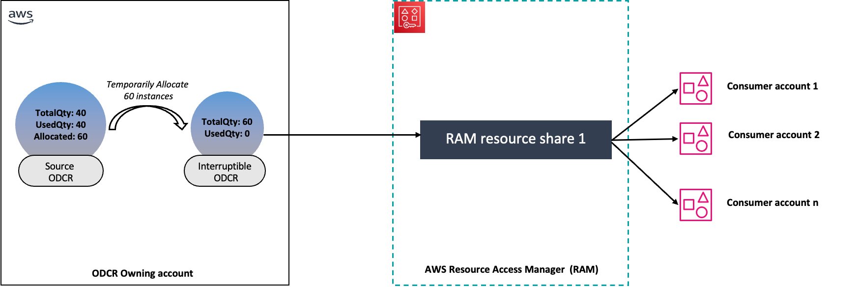
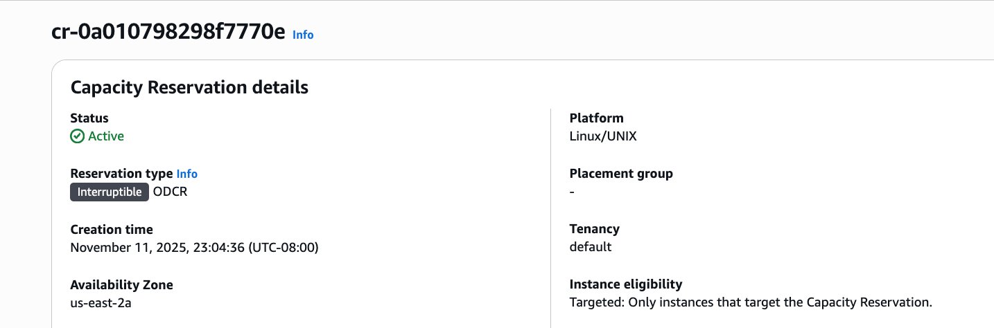
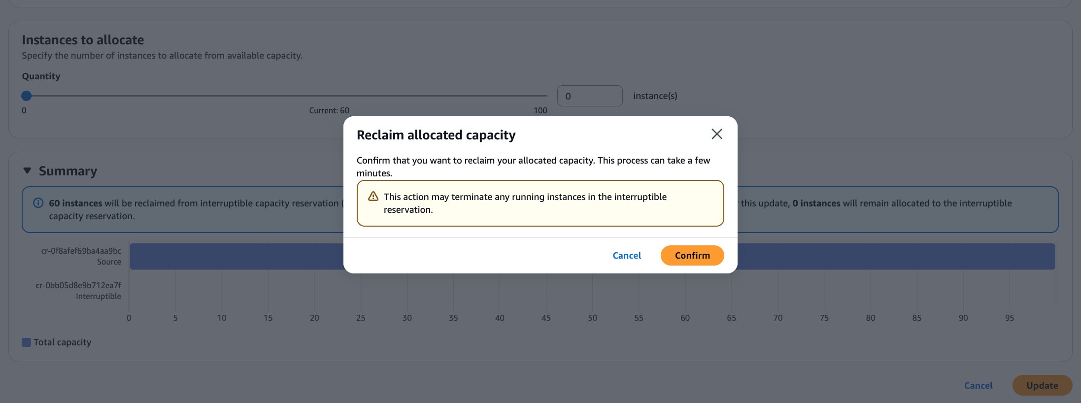
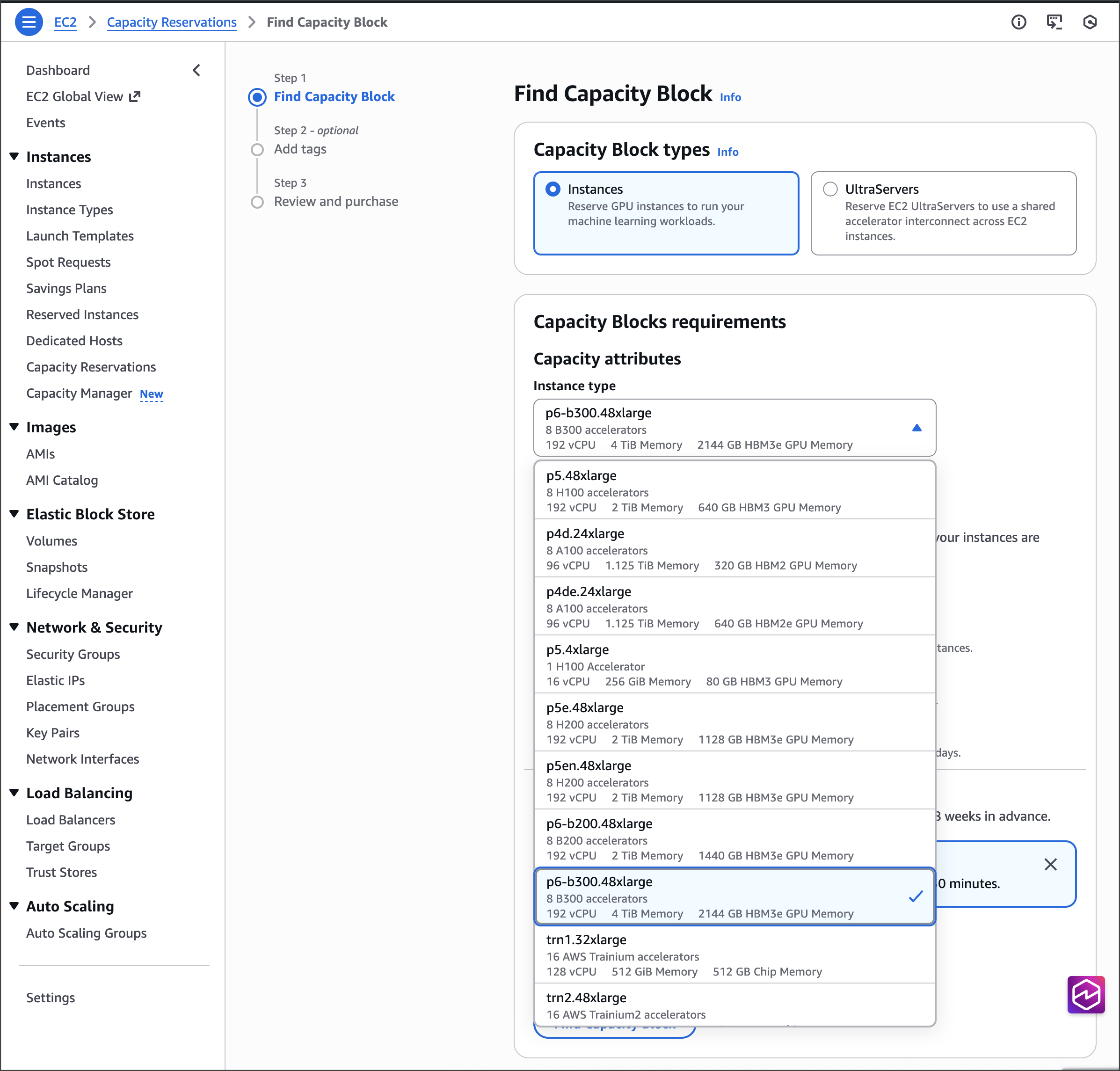
CMP331 | Managing Amazon EC2 capacity and availability
Learn how to optimize EC2 costs and capacity using different reservation models, such as On-Demand, Capacity Blocks for machine learning (ML), and capacity reservations, to improve efficiency and availability.
CMP330 | Use Auto Scaling to proactively scale and optimize EC2 workloads
Learn how to harness the latest features of EC2 Auto Scaling to optimize your cloud resources. This hands-on workshop covers predictive scaling, dynamic scaling, and warm pools to automatically manage capacity based on demand. This is perfect for those wanting to improve application availability while reducing costs. Bring your laptop for practical exercises.
Learn about AWS Compute innovations
AWS has invested years into designing custom silicon optimized for the cloud to deliver the best price performance for a wide range of applications and workloads using AWS services. Learn more about the AWS Nitro System, processors at AWS, and ML chips.
CMP316 | Deep Dive into the AWS Nitro System
Explore the architecture behind the groundbreaking AWS Nitro System: the custom hardware and security components driving modern EC2 instances. Learn how this innovative platform enables unprecedented compute, storage, and networking capabilities, and discover the latest advances making new cloud possibilities reality.
CMP307 | AWS Graviton: The best price performance for your AWS workloads
Explore how AWS Graviton processors deliver superior performance and energy efficiency in EC2. Learn optimization best practices, common use cases, and customer success stories to accelerate your AWS Graviton adoption journey.
CMP336 | Optimize network and Amazon EBS intensive workloads on Amazon EC2 instances
Discover how to maximize the EC2 network and Amazon Elastic Block Store (Amazon EBS)-optimized instances for high-performance workloads. Learn to use new AWS Graviton and Intel instances for security appliances, databases, and network-intensive applications. Get practical insights into the latest networking and storage technologies to optimize your EC2 workload performance.
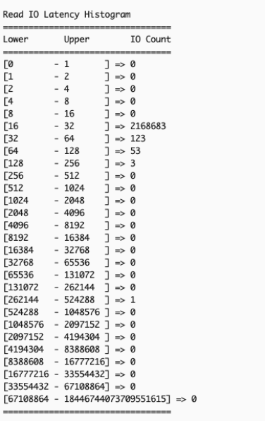
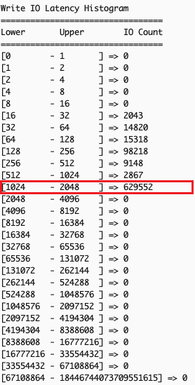
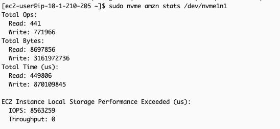
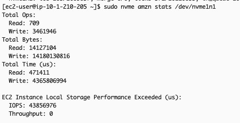
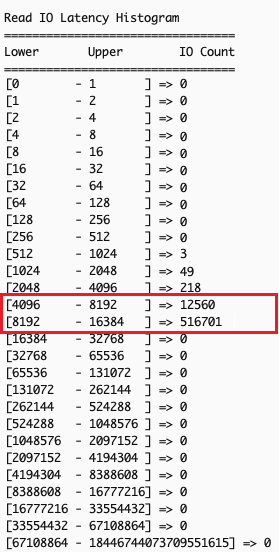
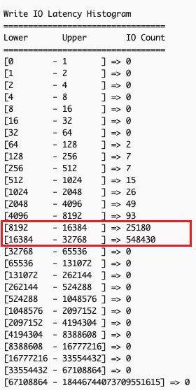
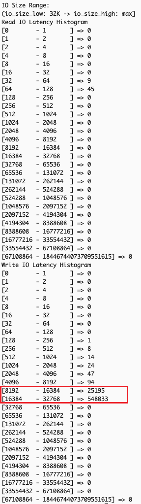
CMP315 | Maximizing EC2 Local NVMe Storage: Enhanced NVMe Metrics and Kubernetes Integration
Learn to optimize data-intensive workloads using AWS Nitro SSDs. Explore new performance metrics (latency, IOPS, throughput) and best practices for monitoring and tuning application performance.
CMP407 | Innovating with AWS confidential computing: An integrated approach
Learn how AWS confidential computing (Nitro System, Enclaves, TPM) protects sensitive data during processing. Explore solutions for secure data handling across CPU, GPU, and AI workloads.
CMP302 | Accelerating engineering: Cross-industry HPC cloud transformations
Discover how AWS high performance computing (HPC) transformed engineering and product development across industries. Learn how customers used cloud HPC to revolutionize their design processes to reduce time-to-market and increase innovation efficiency. Observe how HPC instances, Elastic Fabric Adapter (EFA), Amazon FSx for Lustre, and AWS ParallelCluster accelerate global R&D innovation.
Optimize your compute costs
At AWS, we focus on delivering the best possible cost structure for our customers. Frugality is one of our founding leadership principles. Cost effective design continues to shape everything we do, from how we develop products to how we run our operations. Come learn new ways to optimize your compute costs through AWS services, tools, and optimization strategies in the following sessions:
CMP347 | The Frugal Architect in a chaotic world
Discover the practical implementation of Werner Vogels’ Frugal Architect principles through a hands-on exploration of AWS Graviton, EC2 Spot, Karpenter, and AI tools. Watch as we optimize a shopping cart using AI and flame graphs, demonstrating how to build efficient systems without compromising quality. Learn to combine Karpenter’s intelligent scaling, the performance benefits of AWS Graviton, and AI-driven analysis to create systems that are faster, leaner, and more cost-effective by design.
CMP349 | 5-Star customer service: Duolingo’s path to compute savings
Learn how Duolingo partnered with their AWS Technical Account Manager to transform their cloud spending. Discover their successful transition to AWS Graviton processors, from initial cost analysis through enterprise-wide implementation. Observe how the AWS customer-focused approach delivered significant savings and business value for Duolingo.
CMP337 | Optimizing EC2: Hands-on strategies for cost-effective performance
Get hands-on with advanced EC2 instance optimization in this technical workshop. Learn to analyze workloads, measure performance metrics, and master benchmarking tools through guided exercises. Walk away with practical strategies to choose and tune EC2 instances for your specific application needs. Perfect for architects and developers looking to maximize their AWS infrastructure performance.
CMP314 | Data-driven EC2 optimization: Efficiency, metrics, and sustainability
Join this chalk talk to discover how metric-driven decisions can transform your EC2 fleet optimization. Through real-world scenarios, learn to analyze workload data, choose optimal instance types, and fine-tune capacity for your specific needs. We explore practical approaches to balance cost, performance, and sustainability using AWS-native tools, providing you with actionable strategies that you can implement immediately.
CMP412 | EC2 Flex instances: Get the latest generation performance at lower costs
Explore how EC2 Flex instances deliver the latest generation performance at reduced costs. Learn about optimal workload types, architectural design, and implementation strategies. Discover practical approaches to adoption and performance monitoring to maximize your EC2 Flex instance benefits.
Maximize your workload’s performance
Your workload’s performance matters beyond just cost because it directly impacts the quality, efficiency, and effectiveness of your compute solution. It can significantly influence customer satisfaction, business growth, and overall productivity. Even if a cheaper option exists, a low-cost option with poor performance can lead to long-term financial losses due to issues such as lost customers, engineering rework, and negative reputation. We have several sessions that help you optimize your workload’s performance.
CMP333 | Maximizing EC2 performance: A hands-on guide to instance optimization
Live coding session: Learn to optimize EC2 performance using Amazon CloudWatch and APerf. Observe real-world examples of workload analysis and code optimization across different instance types and programming languages.
CMP351 | Building for efficiency and reliability with performance testing on AWS
Learn performance testing strategies on AWS to optimize costs, identify bottlenecks, and improve reliability. Discover how to measure system behavior under various loads to inform architecture and instance selection decisions.
CMP405 | Everything you’ve wanted to know about performance on EC2 instances
Explore compute optimization techniques in this code talk. Learn about memory topology, hardware counters, hyperthreading effects, and methods for accurate performance testing and latency optimization.
Customer experience and applications with AI and ML
ML has been evolving for decades and has an inflection point with generative AI applications capturing widespread attention and imagination. Learn about generative AI infrastructure at Amazon or get hands-on experience building ML applications through our ML focused sessions, such as the following:
CMP201 | Architecting solution patterns for GPU-accelerated HPC and AI/ML
Interactive discussion on GPU-accelerated HPC and AI/ML architecture. Explore EC2 GPU instance families, architectural tradeoffs , and cost optimization strategies. Share your challenges and learn how to build scalable GPU solutions on AWS.
CMP403 | Build, scale, and optimize agentic AI on CPUs with AWS Graviton
Hands-on workshop: Build cost-efficient AI applications on AWS Graviton. Deploy large language model (LLM) inference, multi-agent systems, and vector databases using Amazon Elastic Kubernetes Service (Amazon EKS) and Karpenter. Create a chat app showcasing the performance benefits of AWS Graviton.
CMP346 | Supercharge ML and inference on Apple Silicon with EC2 Mac
Learn to optimize ML workloads on EC2 Mac instances with Apple silicon. Explore Apple Neural Engine, Core ML, and efficient PyTorch/TensorFlow deployment for iOS and cloud ML applications.
CMP338 | Protect privacy in generative AI applications using AWS Confidential Computing
Build three secure generative AI applications while learning to protect sensitive data in prompts, augmented sources, and model weights. Practice implementing AWS Confidential Computing features in EC2 to mitigate common security threats. Get hands-on experience using both open source models and Amazon Bedrock to create privacy-first AI solutions.
CMP410 | Secure generative AI using trusted execution environments
Hands-on session: Build a secure AI environment using Nitro TPM-enabled EC2 instances. Deploy an LLM with cryptographic attestation and learn to protect sensitive data using trusted execution environments.
Accelerate your AWS Graviton adoption journey
The AWS Graviton Processors are custom designed server processors designed by AWS. They deliver the best price performance for your cloud workloads running in AWS and help you reduce your carbon footprint. Ready to realize up to 40% better price performance for your workloads? We have curated the following session to help you accelerate your AWS Graviton adoption:
CMP329 | Learnings from developers adopting AWS Graviton at scale
Learn how the custom-designed AWS Graviton processors deliver optimal price-performance across diverse workloads: from microservices to HPC. Engage with AWS experts to explore adoption strategies, best practices, and real customer success stories for scaling AWS Graviton in production.
CMP352 | Unlock cost efficiency with AWS Graviton Savings Dashboard
Discover how the enhanced AWS Graviton Savings Dashboard provides deeper analytics for workload modernization, enabling up to 40% better price performance. Learn to use advanced features for granular workload analysis and streamlined migration planning. This lightning talk shows you how to transform efficiency insights into actionable strategies for measurable cloud cost savings.
CMP326 | Java modernization and performance optimization GameDay
Hands-on workshop: Use Amazon Q Developer to modernize Java applications from v8 to v21. Practice automated code analysis, performance benchmarking, and cost optimization across different instances. Laptop needed.
CMP335 | Optimize .NET TCO with agentic AI powered AWS Transform and AWS Graviton
Hands-on workshop: Use agentic AI to accelerate the migration of Windows-based .NET applications to .NET Core running on Linux with AWS Graviton for 40% better price performance. Learn code analysis, automated transformations, and CI/CD updates. For .NET developers/architects. Laptop needed.
Optimizing your container-based workloads
Maximizing the efficiency of container-based workloads is crucial for modern cloud applications. Whether you’re running microservices, web applications, or high-performance computing tasks, optimizing your container infrastructure can significantly impact both performance and cost. In this track, we’ve assembled essential sessions focused on using AWS Graviton processors and modernization tools to enhance your containerized applications. From real-world adoption stories to hands-on workshops, these sessions can help you achieve better price performance while maintaining operational excellence. Join us to explore the following:
CMP310 | Boost Amazon EKS efficiency: Amazon EKS Auto Mode, AWS Graviton, and EC2 Spot
Explore how Amazon EKS Auto Mode streamlines Kubernetes operations by removing infrastructure management complexity. Learn to optimize costs using AWS Graviton and EC2 Spot, with practical examples for building more efficient, cost-effective container environments.
CMP311 | Build once, run everywhere: Multi-architecture in your CI/CD pipelines
Learn to build multi-architecture containers for x86 and AWS Graviton processors. Observe how to optimize web applications for both platforms and integrate with CI/CD systems such as ArgoCD, GitLab, and GitHub.
CMP348 | Using Amazon Q to cost optimize your containerized workloads
Learn to achieve 40% better price-performance by migrating containerized workloads to AWS Graviton using Amazon EKS and Karpenter. Use Amazon Q to accelerate x86-to-Graviton migration, implement multi-architecture CI/CD pipelines, and optimize deployment strategies.
Quantum computing
Quantum computing is moving from theoretical possibility to practical reality, offering groundbreaking potential across industries. As organizations prepare for this technology, AWS provides the tools and infrastructure needed to explore quantum applications today. Through Amazon Braket, our managed quantum computing service, we’re making quantum experimentation accessible to enterprises, researchers, and developers alike. Whether you’re interested in drug discovery, optimization problems, or cybersecurity, this track offers a comprehensive journey from quantum basics to advanced hybrid solutions. Join industry leaders, such as AstraZeneca and Accenture, to discover how quantum computing is already delivering value and how you can begin your quantum journey:
CMP202 | Amazon Braket: Get hands-on with quantum computing
Get started with quantum computing in this practical workshop. Learn to implement quantum algorithms and run circuits on gate-based devices using Amazon Braket. Explore the quantum algorithm library of AWS through hands-on exercises. Bring your laptop to begin your quantum journey.
CMP209 | Amazon Braket hubs: Accelerating R&D in national quantum initiatives
Learn how AWS supports quantum computing research hubs worldwide, helping create secure environments and providing access to cutting-edge quantum technologies for researchers and startups.
CMP411 | Quantum computing with Amazon Braket: From exploration to enterprise
Explore quantum computing with Amazon Braket, featuring the AWS strategy and AstraZeneca’s drug discovery research. Learn how to combine quantum and classical workloads and prepare for future quantum technologies.
CMP205 | Q-CTRL Fire Opal on Amazon Braket: Quantum solutions from security to finance
Learn how organizations use Q-CTRL and Amazon Braket for quantum computing breakthroughs. Observe how Accenture Federal Services achieved 3x better network security detection using Q-CTRL’s optimizer, and explore quantum-classical solutions for various industries.
CMP304 | Architectures for hybrid quantum-classical workflows at scale
Learn to build hybrid quantum-classical computing solutions using Amazon Braket with AWS services (AWS Batch, AWS ParallelCluster) and GPU-accelerated instances. Explore architectures integrating CPUs, GPUs, and quantum processors using NVIDIA CUDA-Q.
Check out workload-specific sessions
EC2 offers the broadest and deepest compute platform to help you best match the needs of your workload. Join sessions focused on your specific workload to learn about how you can use AWS solutions to accelerate your innovations.
CMP207 | Startup to scale: Powering business growth with Amazon Lightsail
Get started in the cloud with just a few clicks with Amazon Lightsail. Discover how it can support your business at any stage of growth. Whether you’re launching your first cloud workload, migrating existing applications, or managing services for your customers, learn proven approaches for success. We explore how customers are using Lightsail today, including cost optimization and best practices for efficient scaling.
CMP320 | Full stack web apps on EC2: Using AWS Elastic Beanstalk with Amazon Q
Accelerate your cloud journey with AWS Elastic Beanstalk and Amazon Q. Learn how Elastic Beanstalk streamlines deployment and maintenance of full stack web applications on EC2 with automated infrastructure provisioning, while Amazon Q enhances your Elastic Beanstalk experience with natural language commands, intelligent troubleshooting guidance, and deployment best practices recommendations. This is perfect for teams ready to focus on building exceptional applications instead of managing infrastructure.
CMP334 | Modernize Apple platform development with AWS and EC2 Mac
Explore how EC2 Mac instances enable scalable, cost-effective macOS workloads on AWS. Learn about the latest features and hear a customer success story showcasing optimized Apple development workflows in the cloud.
CMP341 | SAP workloads on memory optimized Amazon EC2 instances
Discover how the memory-optimized instances (R, X, U) of EC2 revolutionize SAP HANA deployments, eliminating traditional infrastructure compromises. Learn from SAP’s experience managing RISE with SAP on AWS, and explore how high-memory instances can transform your SAP operations.
CMP319 | Exploring the spectrum of architecture patterns for 3D rendering
Explore the complete rendering toolkit of AWS for 3D and spatial applications: from GPU-powered EC2 instances to distributed rendering with Deadline Cloud and real-time GameLift Streams. Learn practical architecture patterns and cost optimization strategies to scale your rendering pipeline for games, architectural visualization, and AR/VR experiences.
CMP321 | Generative AI storyboarding: From Sketch to 3D Scene with generative AI on AWS
Learn to create visual content using Amazon Bedrock: convert sketches to storyboards, generate 2D/3D assets, and compose scenes. Explore AI-assisted workflows for film, games, and UI design while maintaining artistic control.
CMP211 | Hybrid science: AI + physics simulations for climate and life sciences
Explore how to combine AI with physics simulations using AWS services (such as AWS Batch, AWS ParallelCluster, Amazon FSx, EFA). Learn real-world patterns for integrating AI and simulation workflows in climate, weather, and healthcare applications.
CMP345 | Accelerate drug discovery R&D at scale with AWS
Interactive session on how top pharma companies use AWS for drug discovery R&D. Explore solutions for imaging, molecular simulation, and AI-driven research, with focus on managing large-scale data and diverse compute needs.
CMP350 | Accelerating vehicle innovation: ML and HPC best practices
Learn how Toyota and Deloitte transformed automotive engineering by migrating HPC and ML workloads to AWS. Using NVIDIA GPUs and EC2 HPC instances, they dramatically reduced development cycles. You can gain practical insights for your own high-performance computing initiatives.
CMP401 | Accelerating semiconductor design, simulation, and verification on AWS
This session covers the latest compute and storage innovations such as the new generation of EC2 instances powered by custom Intel Xeon Scalable processors (Granite Rapids), AMD EPYC processors (Turin), and AWS Graviton, and new features of Amazon FSx for NetApp ONTAP.
CMP406 | HPC infrastructure for financial services using AWS Batch and AWS CDK
Hands-on session: Build HPC infrastructure using AWS Cloud Development Kit (AWS CDK). Deploy AWS Batch for financial risk analysis workloads. This is suitable for HPC experts new to AWS and AWS developers new to HPC.
CMP204 | Quantum computing: Accelerating pharma innovation
Explore how Merck Sharp & Dohme partners with MathWorks and AWS to revolutionize pharmaceutical development through quantum computing. Using MATLAB and Amazon Braket, they implement QAOA for optimizing drug production and enhancing cancer diagnostics.
Ready to unlock new possibilities?
The AWS Compute team looks forward to seeing you in Las Vegas. Come meet us at the Compute Booth in the Expo and check out our various EC2 demos. And if you’re looking for more session recommendations, check-out more re:Invent attendee guides curated by experts.