Linux malware often hides in Berkeley Packet Filter (BPF) socket programs, which are small bits of executable logic that can be embedded in the Linux kernel to customize how it processes network traffic. Some of the most persistent threats on the Internet use these filters to remain dormant until they receive a specific “magic” packet. Because these filters can be hundreds of instructions long and involve complex logical jumps, reverse-engineering them by hand is a slow process that creates a bottleneck for security researchers.
To find a better way, we looked at symbolic execution: a method of treating code as a series of constraints, rather than just instructions. By using the Z3 theorem prover, we can work backward from a malicious filter to automatically generate the packet required to trigger it. In this post, we explain how we built a tool to automate this, turning hours of manual assembly analysis into a task that takes just a few seconds.
The complexity ceiling
Before we look at how to deconstruct malicious filters, we need to understand the engine running them. The Berkeley Packet Filter (BPF) is a highly efficient technology that allows the kernel to pull specific packets from the network stack based on a set of bytecode instructions.
While many modern developers are familiar with eBPF (Extended BPF), the powerful evolution used for observability and security, this post focuses on “classic” BPF. Originally designed for tools like tcpdump, classic BPF uses a simple virtual machine with just two registers to evaluate network traffic at high speeds. Because it runs deep within the kernel and can “hide” traffic from user-space tools, it has become a favorite tool for malware authors looking to build stealthy backdoors.
Creating a contextual representation of BPF instructions using LLMs is already reducing the manual overhead for analysts, crafting the network packets that correspond to the validating condition can still be a lot of work, even with the added context provided by LLM’s.
Most of the time this is not a problem if your BPF program has only ~20 instructions, but this can get exponentially more complex and time-consuming when a BPF program consists of over 100 instructions as we’ve observed in some of the samples.
If we deconstruct the problem we can see that it boils down to reading a buffer and checking a constraint, depending on the outcome we either continue our execution path or stop and check the end result.
This kind of problem that has a deterministic outcome can be solved by Z3, a theorem prover that has the means to solve problems with a set of given constraints.
Exhibit A: BPFDoor
BPFDoor is a sophisticated, passive Linux backdoor, primarily used for cyberespionage by China-based threat actors, including Red Menshen (also known as Earth Bluecrow). Active since at least 2021, the malware is designed to maintain a stealthy foothold in compromised networks, targeting telecommunications, education, and government sectors, with a strong emphasis on operations in Asia and the Middle East.
BPFDoor uses BPF to monitor all incoming traffic without requiring a specific network port to be open.
BPFDoor example instructions
Let’s focus on the sample of which was shared for the research done by Fortinet (82ed617816453eba2d755642e3efebfcbd19705ac626f6bc8ed238f4fc111bb0). If we dissect the BPF instructions and add some annotations, we can write the following:
(000) ldh [0xc]                   ; Read halfword at offset 12 (EtherType)
(001) jeq #0x86dd, jt 2, jf 6     ; 0x86DD (IPv6) -> ins 002 else ins 006
(002) ldb [0x14]                  ; Read byte at offset 20 (Protocol)
(003) jeq #0x11, jt 4, jf 15      ; 0x11 (UDP) -> ins 004 else DROP
(004) ldh [0x38]                  ; Read halfword at offset 56 (Dst Port)
(005) jeq #0x35, jt 14, jf 15     ; 0x35 (DNS) -> ACCEPT else DROP
(006) jeq #0x800, jt 7, jf 15     ; 0x800 (IPv4) -> ins 007 else DROP
(007) ldb [23]                    ; Read byte at offset 23 (Protocol)
(008) jeq #0x11, jt 9, jf 15      ; 0x11 (UDP) -> ins 009 else DROP
(009) ldh [20]                    ; Read halfword at offset 20 (fragment)
(010) jset #0x1fff, jt 15, jf 11  ; fragmented -> DROP else ins 011
(011) ldxb 4*([14]&0xf)           ; Load index (x) register ihl & 0xf
(012) ldh [x + 16]                ; Read halfword at offset x+16 (Dst Port)
(013) jeq #0x35, jt 14, jf 15     ; 0x35 (DNS) -> ACCEPT else DROP
(014) ret #0x40000 (ACCEPT)
(015) ret #0 (DROP)
In the above example we can establish there are two paths that lead to an ACCEPT outcome (step 5 and step 13). We can also clearly observe certain bytes being checked, including their offsets and values.
Taking these validations, and keeping track of anything that would match the ACCEPT path, we should be able to automatically craft the packets for us.
Calculating the shortest path
To find the shortest path to a packet that validates the conditions presented in the BPF instructions, we need to keep track of paths that are not ending in the unfavorable condition.
We start off by creating a small queue. This queue holds several important data points:
The pointer to the next instruction.
Our current path of executed instructions + the next instruction.
Whenever we encounter an instruction that is checking a condition, we keep track of the outcome using a boolean and store this in our queue, so we can compare paths on the amount of conditions before the ACCEPT condition is reached and calculate our shortest path. In pseudocode we can express this best as:
paths = []
queue = dequeue([(0, [0])])

while queue:
	pc, path = queue.popleft()

	if pc >= len(instructions):
            continue

instruction = instructions[pc]

	if instruction.class == return_instruction:
		if instruction_constant != 0:  # accept
			paths.append(path)
		continue  # drop or accept, stop parsing this instruction

if instruction.class == jump_instruction:
	if instruction.operation == unconditional_jump:
		next_pc = pc + 1 + instruction_constant
		queue.append((next_pc, path + [next_pc]))
		continue

	# Conditional jump, explore both
	pc_true = pc + 1 + instruction.jump_true
	pc_false = pc + 1 + instruction.jump_false

	if instruction.jump_true <= instruction.jump_false:
		queue.append((pc_true, path + [pc_true]))
		queue.append((pc_false, path + [pc_false]))
	# else: same as above but reverse order of appending
# else: sequential instruction, append to the queue
If we execute this logic against our earlier BPFDoor example, we will be presented with the shortest path to an accepted packet:
This is already a helpful automation in automatically solving our BPF constraints when it comes to analyzing BPF instructions and figuring out how the accepted packet for the backdoor would look. But what if we can take it a step further?
What if we could create a small tool that will give us the expected packet back in an automated manner?
Employing Z3 and scapy
One such tool that is perfect to solve problems given a set of constraints is Z3. Developed by Microsoft the tool is labeled as a theorem prover and exposes easy to use functions performing very complex mathematical operations under the hood.
The other tool we will use for crafting our valid magic packets is scapy, a popular Python library for interactive packet manipulation.
Given that we already have a way to figure out the path to an accepted packet, we are left with solving the problem by itself, and then translating this solution to the bytes at their respective offsets in a network packet.
Symbolic execution
A common technique for exploring paths taken in a given program is called symbolic execution. For this technique we are giving input that can be used as variables, including the constraints. By knowing the outcome of a successful path we can orchestrate our tool to find all of these successful paths and display the end result to us in a contextualized format.
For this to work we will need to implement a small machine capable of keeping track of the state of things like constants, registers, and different boolean operators as an outcome of a condition that is being checked.
class BPFPacketCrafter:
    MIN_PKT_SIZE = 64           # Minimum packet size (Ethernet + IP + UDP headers)
    LINK_ETHERNET = "ethernet"  # DLT_EN10MB - starts with Ethernet header
    LINK_RAW = "raw"            # DLT_RAW - starts with IP header directly
    MEM_SLOTS = 16              # Number of scratch memory slots (M[0] to M[15])

    def __init__(self, ins: list[BPFInsn], pkt_size: int = 128, ltype: str = "ethernet"):
        self.instructions = ins
        self.pkt_size = max(self.MIN_PKT_SIZE, pkt_size)
        self.ltype = ltype

        # Symbolic packet bytes
        self.packet = [BitVec(f"pkt_{i}", 8) for i in range(self.pkt_size)]

        # Symbolic registers (32-bit)
        self.A = BitVecVal(0, 32)  # Accumulator
        self.X = BitVecVal(0, 32)  # Index register

        # Scratch memory M[0-15] (32-bit words)
        self.M = [BitVecVal(0, 32) for _ in range(self.MEM_SLOTS)]
With the above code we’ve covered most of the machine for keeping a state during the symbolic execution. There are of course more conditions we need to keep track of, but these are handled during the solving process. To handle an ADD instruction, the machine maps the BPF operation to a Z3 addition:
def _execute_ins(self, insn: BPFInsn):
    cls = insn.cls
    if cls == BPFClass.ALU:
        op = insn.op
        src_val = BitVecVal(insn.k, 32) if insn.src == BPFSrc.K else self.X
        if op == BPFOp.ADD:
            self.A = self.A + src_val
Luckily the BPF instruction set is only a small set of instructions that’s relatively easy to implement — only having two registers to keep track of is definitely a welcome constraint!
The overall working of this symbolic execution can be laid out in the following abstracted overview:
Initialize the “x” (index) and “a” (accumulator) registers to their base state.
Loop over the instructions from the path that was identified as a successful path;
Execute non-jump instructions as-is, keeping track of register states.
Determine if a jump instruction is encountered, and check if the branch should be taken.
Use the Z3 check() function to check if our condition has been satisfied with the given constraint (ACCEPT).
Convert the Z3 bitvector arrays into bytes.
Use scapy to construct packets of the converted bytes.
If we look at the constraints build by the Z3 solver we can trace the execution steps taken by Z3 to build the packet bytes:
The first part of the Z3 displayed constraints are the constraints added to ensure we’re building up a valid ethernet IP when dealing with link-layer BPF instructions. The “If” statements apply specific constraints based on which protocol is detected:
IPv4 Logic (0x0800):
pkt_14 & 240 == 64: Byte 14 is the start of the IP header. The 0xF0 mask isolates the high nibble (the Version field) to check if the version is 4 (0x40).
pkt_14 & 15 == 5: 15 (0x0F), isolating the low nibble (IHL – Internet Header Length). This mandates a header length of 5 (20 bytes), which is the standard size without options.
IPv6 Logic (0x86dd):
pkt_14 & 240 == 0x60: Check if the version field is version 6 (0x60)
We can observe the network packet values when we look at the second part where different values are being checked:
0x86DD: Packet condition for IPv6 header.
0x11: UDP protocol number.
0x35: The destination port (53).
Next to the expected values we can see the byte offset of where it should exist in a given packet (e.g. pkt_12, pkt_13).
Crafting packets
Now that we’ve established which bytes should exist at specific offsets we can convert it into an actual network packet using scapy. If we generate a new packet from the bytes of our previous Z3 constraints we can clearly see what our packet would look like, and store this for further processing:
These newly crafted packets can in turn be used for further research or identifying the presence of these implants by scanning for these over the network.
Try it yourself
Understanding what a specific BPF set of instructions is doing can be cumbersome and time-consuming work. The example used is only a total of sixteen instructions, but we’ve encountered samples that were over 200 instructions that would’ve taken at least a day to understand. By using the Z3 solver, we can now reduce this time to just seconds, and not only display the path to an accepted packet, but also the packet skeleton for this as well.
We have open-sourced the filterforge tool to help the community automate the deconstruction of BPF-based implants. You can find the source code, along with usage examples, on our GitHub repository.
By publishing this research and sharing our tool for reducing analysts’ time spent figuring out the BPF instructions, we hope to spark further research by others to expand on this form of automation.
Early on when we learn to program, we get introduced to the concept of recursion. And that it is handy for computing, among other things, sequences defined in terms of recurrences. Such as the famous Fibonnaci numbers – Fn = Fn-1 + Fn-2.
Later on, perhaps when diving into multithreaded programming, we come to terms with the fact that the stack space for call frames is finite. And that there is an “okay” way and a “cool” way to calculate the Fibonacci numbers using recursion:
This has an important consequence – as fib recursively calls itself, the stacks keep growing. We can observe it with a bit of help from the debugger.
$ gdb --quiet --batch --command=trace_rsp.gdb --args ./fib_okay 6
Breakpoint 1 at 0x401188: file fib_okay.c, line 3.
[Thread debugging using libthread_db enabled]
Using host libthread_db library "/lib64/libthread_db.so.1".
n = 6, %rsp = 0xffffd920
n = 5, %rsp = 0xffffd900
n = 4, %rsp = 0xffffd8e0
n = 3, %rsp = 0xffffd8c0
n = 2, %rsp = 0xffffd8a0
n = 1, %rsp = 0xffffd880
n = 1, %rsp = 0xffffd8c0
n = 2, %rsp = 0xffffd8e0
n = 1, %rsp = 0xffffd8c0
n = 3, %rsp = 0xffffd900
n = 2, %rsp = 0xffffd8e0
n = 1, %rsp = 0xffffd8c0
n = 1, %rsp = 0xffffd900
13
[Inferior 1 (process 50904) exited normally]
$
While the “cool” variant makes no use of the stack.
$ gdb --quiet --batch --command=trace_rsp.gdb --args ./fib_cool 6
Breakpoint 1 at 0x40118a: file fib_cool.c, line 13.
[Thread debugging using libthread_db enabled]
Using host libthread_db library "/lib64/libthread_db.so.1".
n = 6, %rsp = 0xffffd938
13
[Inferior 1 (process 50949) exited normally]
$
Where did the calls go?
The smart compiler turned the last function call in the body into a regular jump. Why was it allowed to do that?
It is the last instruction in the function body we are talking about. The caller stack frame is going to be destroyed right after we return anyway. So why keep it around when we can reuse it for the callee’s stack frame?
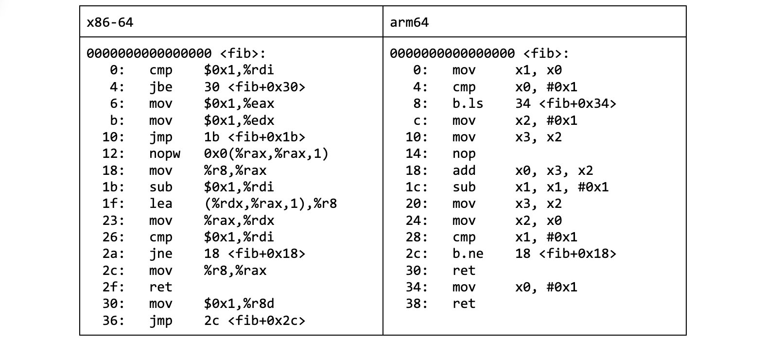
This optimization, known as tail call elimination, leaves us with no function calls in the “cool” variant of our fib implementation. There was only one call to eliminate – right at the end.
Once applied, the call becomes a jump (loop). If assembly is not your second language, decompiling the fib_cool.o object file with Ghidra helps see the transformation:
long fib(ulong param_1)

{
  long lVar1;
  long lVar2;
  long lVar3;

  if (param_1 < 2) {
    lVar3 = 1;
  }
  else {
    lVar3 = 1;
    lVar2 = 1;
    do {
      lVar1 = lVar3;
      param_1 = param_1 - 1;
      lVar3 = lVar2 + lVar1;
      lVar2 = lVar1;
    } while (param_1 != 1);
  }
  return lVar3;
}
Listing 4. fib_cool.o decompiled by Ghidra
This is very much desired. Not only is the generated machine code much shorter. It is also way faster due to lack of calls, which pop up on the profile for fib_okay.
But I am no performance ninja and this blog post is not about compiler optimizations. So why am I telling you about it?
The concept of tail call elimination made its way into the BPF world. Although not in the way you might expect. Yes, the LLVM compiler does get rid of the trailing function calls when building for -target bpf. The transformation happens at the intermediate representation level, so it is backend agnostic. This can save you some BPF-to-BPF function calls, which you can spot by looking for call -N instructions in the BPF assembly.
However, when we talk about tail calls in the BPF context, we usually have something else in mind. And that is a mechanism, built into the BPF JIT compiler, for chaining BPF programs.
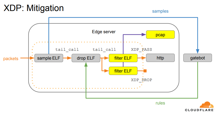
We first adopted BPF tail calls when building our XDP-based packet processing pipeline. Thanks to it, we were able to divide the processing logic into several XDP programs. Each responsible for doing one thing.
BPF tail calls have served us well since then. But they do have their caveats. Until recently it was impossible to have both BPF tails calls and BPF-to-BPF function calls in the same XDP program on arm64, which is one of the supported architectures for us.
Why? Before we get to that, we have to clarify what a BPF tail call actually does.
A tail call is a tail call is a tail call
BPF exposes the tail call mechanism through the bpf_tail_call helper, which we can invoke from our BPF code. We don’t directly point out which BPF program we would like to call. Instead, we pass it a BPF map (a container) capable of holding references to BPF programs (BPF_MAP_TYPE_PROG_ARRAY), and an index into the map.
long bpf_tail_call(void *ctx, struct bpf_map *prog_array_map, u32 index)

       Description
              This  special  helper is used to trigger a "tail call", or
              in other words, to jump into  another  eBPF  program.  The
              same  stack frame is used (but values on stack and in reg‐
              isters for the caller are not accessible to  the  callee).
              This  mechanism  allows  for  program chaining, either for
              raising the maximum number of available eBPF instructions,
              or  to  execute  given programs in conditional blocks. For
              security reasons, there is an upper limit to the number of
              successive tail calls that can be performed.
At first glance, this looks somewhat similar to the execve(2) syscall. It is easy to mistake it for a way to execute a new program from the current program context. To quote the excellent BPF and XDP Reference Guide from the Cilium project documentation:
Tail calls can be seen as a mechanism that allows one BPF program to call another, without returning to the old program. Such a call has minimal overhead as unlike function calls, it is implemented as a long jump, reusing the same stack frame.
But once we add BPF function calls into the mix, it becomes clear that the BPF tail call mechanism is indeed an implementation of tail call elimination, rather than a way to replace one program with another:
Tail calls, before the actual jump to the target program, will unwind only its current stack frame. As we can see in the example above, if a tail call occurs from within the sub-function, the function’s (func1) stack frame will be present on the stack when a program execution is at func2. Once the final function (func3) function terminates, all the previous stack frames will be unwinded and control will get back to the caller of BPF program caller.
Alas, one with sometimes slightly surprising semantics. Consider the code like below, where a BPF function calls the bpf_tail_call() helper:
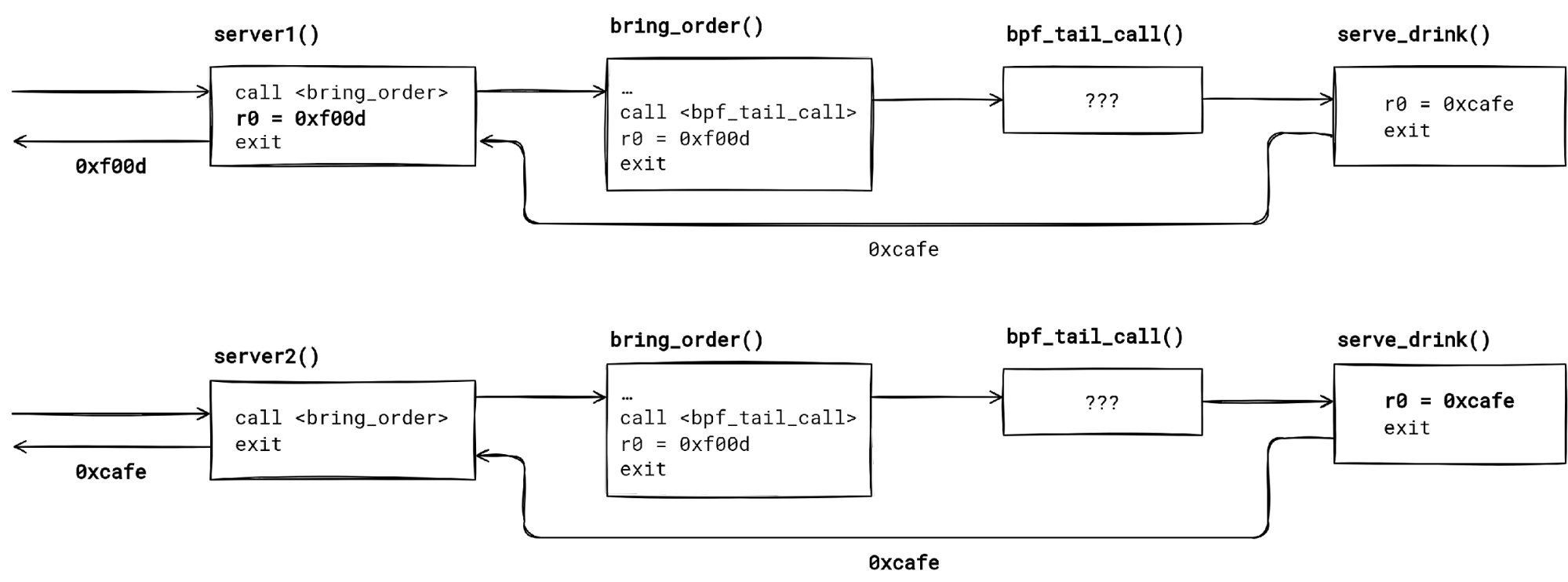
We have two seemingly not so different BPF programs – server1() and server2(). They both call the same BPF function bring_order(). The function tail calls into the serve_drink() program, if the bar[0] map entry points to it (let’s assume that).
Do both server1 and server2 return the same value? Turns out that – no, they don’t. We get a hex 🍔 from server1, and a ☕ from server2. How so?
First thing to notice is that a BPF tail call unwinds just the current function stack frame. Code past the bpf_tail_call() invocation in the function body never executes, providing the tail call is successful (the map entry was set, and the tail call limit has not been reached).
When the tail call finishes, control returns to the caller of the function which made the tail call. Applying this to our example, the control flow is serverX() --> bring_order() --> bpf_tail_call() --> serve_drink() -return-> serverX() for both programs.
The second thing to keep in mind is that the compiler does not know that the bpf_tail_call() helper changes the control flow. Hence, the unsuspecting compiler optimizes the code as if the execution would continue past the BPF tail call.
The call graph for server1() and server2() is the same, but the return value differs due to build time optimizations.
In our case, the compiler thinks it is okay to propagate the constant which bring_order() returns to server1(). Possibly catching us by surprise, if we didn’t check the generated BPF assembly.
We can prevent it by forcing the compiler to make a tail call to bring_order(). This way we ensure that whatever bring_order() returns will be used as the server2() program result.
🛈 General rule – for least surprising results, use musttail attribute when calling a function that contain a BPF tail call.
How does the bpf_tail_call() work underneath then? And why the BPF verifier wouldn’t let us mix the function calls with tail calls on arm64? Time to dig deeper.
What does a bpf_tail_call() helper call translate to after BPF JIT for x86-64 has compiled it? How does the implementation guarantee that we don’t end up in a tail call loop forever?
To find out we will need to piece together a few things.
First, there is the BPF JIT compiler source code, which lives in arch/x86/net/bpf_jit_comp.c. Its code is annotated with helpful comments. We will focus our attention on the following call chain within the JIT:
It is sometimes hard to visualize the generated instruction stream just from reading the compiler code. Hence, we will also want to inspect the input – BPF instructions – and the output – x86-64 instructions – of the JIT compiler.
To inspect BPF and x86-64 instructions of a loaded BPF program, we can use bpftool prog dump. However, first we must populate the BPF map used as the tail call jump table. Otherwise, we might not be able to see the tail call jump!
This is due to optimizations that use instruction patching when the index into the program array is known at load time.
There is a caveat. The target addresses for tail call jumps in bpftool prog dump jited output will not make any sense. To discover the real jump targets, we have to peek into the kernel memory. That can be done with gdb after we find the address of our JIT’ed BPF programs in /proc/kallsyms:
Lastly, it will be handy to have a cheat sheet of mapping between BPF registers (r0, r1, …) to hardware registers (rax, rdi, …) that the JIT compiler uses.
BPF
x86-64
r0
rax
r1
rdi
r2
rsi
r3
rdx
r4
rcx
r5
r8
r6
rbx
r7
r13
r8
r14
r9
r15
r10
rbp
internal
r9-r12
Now we are prepared to work out what happens when we use a BPF tail call.
In essence, bpf_tail_call() emits a jump into another function, reusing the current stack frame. It is just like a regular optimized tail call, but with a twist.
Because of the BPF security guarantees – execution terminates, no stack overflows – there is a limit on the number of tail calls we can have (MAX_TAIL_CALL_CNT = 33).
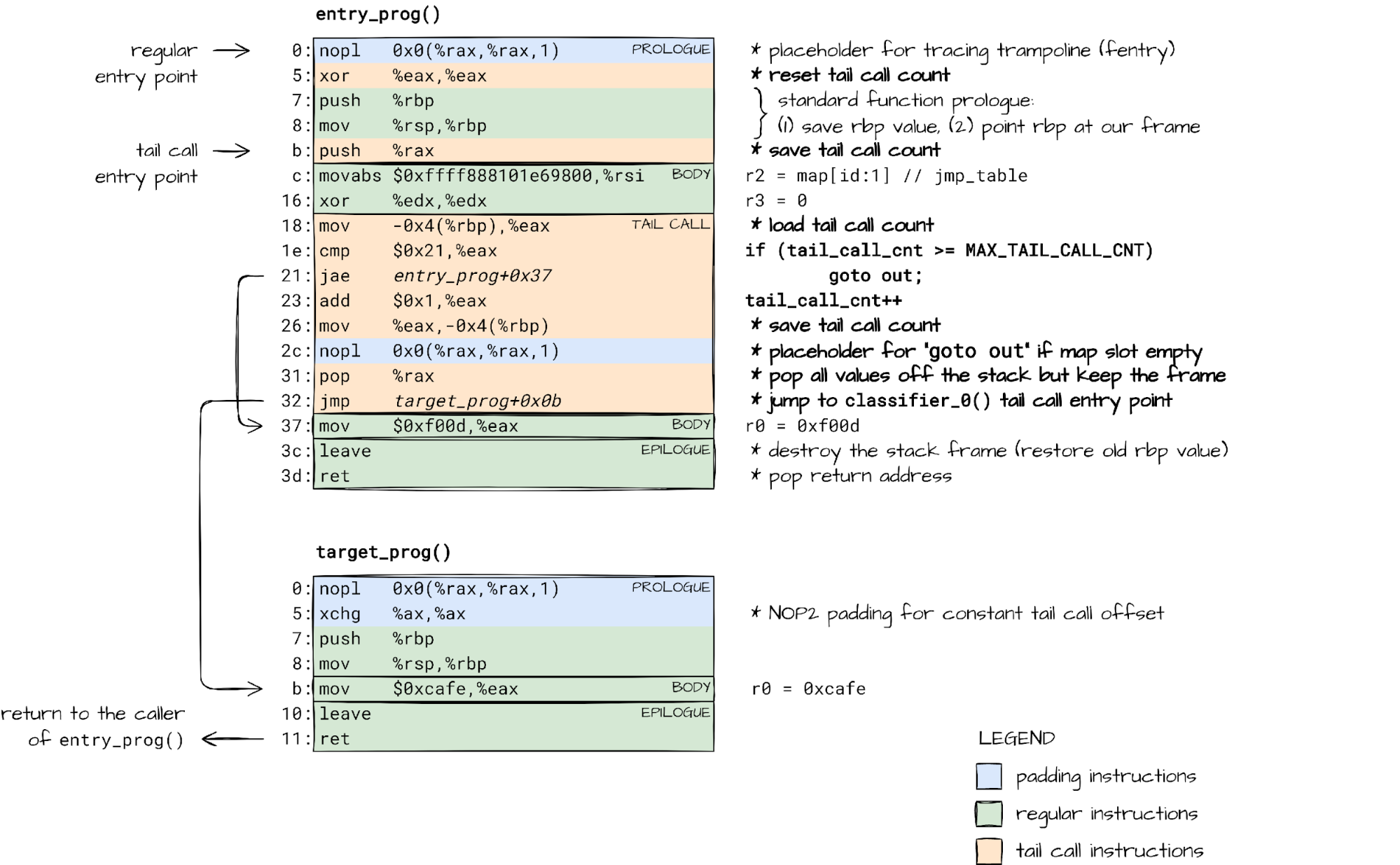
Counting the tail calls across BPF programs is not something we can do at load-time. The jump table (BPF program array) contents can change after the program has been verified. Our only option is to keep track of tail calls at run-time. That is why the JIT’ed code for the bpf_tail_call() helper checks and updates the tail_call_cnt counter.
The updated count is then passed from one BPF program to another, and from one BPF function to another, as we will see, through the rax register (r0 in BPF).
Luckily for us, the x86-64 calling convention dictates that the rax register does not partake in passing function arguments, but rather holds the function return value. The JIT can repurpose it to pass an additional – hidden – argument.
The function body is, however, free to make use of the r0/rax register in any way it pleases. This explains why we want to save the tail_call_cnt passed via rax onto stack right after we jump to another program. bpf_tail_call() can later load the value from a known location on the stack.
This way, the code emitted for each bpf_tail_call() invocation, and the BPF function prologue work in tandem, keeping track of tail call count across BPF program boundaries.
But what if our BPF program is split up into several BPF functions, each with its own stack frame? What if these functions perform BPF tail calls? How is the tail call count tracked then?
Mixing BPF function calls with BPF tail calls
BPF has its own terminology when it comes to functions and calling them, which is influenced by the internal implementation. Function calls are referred to as BPF to BPF calls. Also, the main/entry function in your BPF code is called “the program”, while all other functions are known as “subprograms”.
Each call to subprogram allocates a stack frame for local state, which persists until the function returns. Naturally, BPF subprogram calls can be nested creating a call chain. Just like nested function calls in user-space.
BPF subprograms are also allowed to make BPF tail calls. This, effectively, is a mechanism for extending the call chain to another BPF program and its subprograms.
static int check_max_stack_depth(struct bpf_verifier_env *env)
{
        …
        /* protect against potential stack overflow that might happen when
         * bpf2bpf calls get combined with tailcalls. Limit the caller's stack
         * depth for such case down to 256 so that the worst case scenario
         * would result in 8k stack size (32 which is tailcall limit * 256 =
         * 8k).
         *
         * To get the idea what might happen, see an example:
         * func1 -> sub rsp, 128
         *  subfunc1 -> sub rsp, 256
         *  tailcall1 -> add rsp, 256
         *   func2 -> sub rsp, 192 (total stack size = 128 + 192 = 320)
         *   subfunc2 -> sub rsp, 64
         *   subfunc22 -> sub rsp, 128
         *   tailcall2 -> add rsp, 128
         *    func3 -> sub rsp, 32 (total stack size 128 + 192 + 64 + 32 = 416)
         *
         * tailcall will unwind the current stack frame but it will not get rid
         * of caller's stack as shown on the example above.
         */
        if (idx && subprog[idx].has_tail_call && depth >= 256) {
                verbose(env,
                        "tail_calls are not allowed when call stack of previous frames is %d bytes. Too large\n",
                        depth);
                return -EACCES;
        }
        …
}
While the stack depth can be calculated by the BPF verifier at load-time, we still need to keep count of tail call jumps at run-time. Even when subprograms are involved.
This means that we have to pass the tail call count from one BPF subprogram to another, just like we did when making a BPF tail call, so we yet again turn to value passing through the rax register.
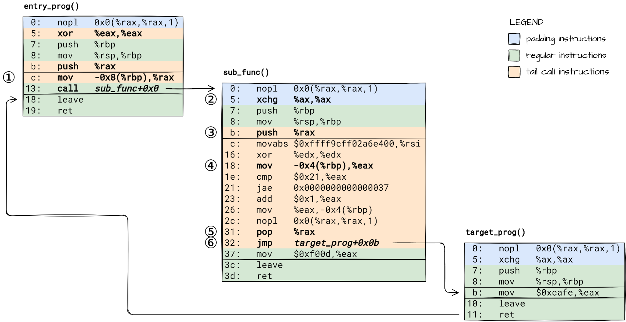
Control flow in a BPF program with a function call followed by a tail call.
🛈 To keep things simple, BPF code in our examples does not allocate anything on stack. I encourage you to check how the JIT’ed code changes when you add some local variables. Just make sure the compiler does not optimize them out.
To make it work, we need to:
① load the tail call count saved on stack into rax before call’ing the subprogram, ② adjust the subprogram prologue, so that it does not reset the rax like the main program does, ③ save the passed tail call count on subprogram’s stack for the bpf_tail_call() helper to consume it.
A bpf_tail_call() within our suprogram will then:
④ load the tail call count from stack, ⑤ unwind the BPF stack, but keep the current subprogram’s stack frame in tact, and ⑥ jump to the target BPF program.
Now we have seen how all the pieces of the puzzle fit together to make BPF tail work on x86-64 safely. The only open question is does it work the same way on other platforms like arm64? Time to shift gears and dive into a completely different BPF JIT implementation.
If you try loading a BPF program that uses both BPF function calls (aka BPF to BPF calls) and BPF tail calls on an arm64 machine running the latest 5.15 LTS kernel, or even the latest 5.19 stable kernel, the BPF verifier will kindly ask you to reconsider your choice:
That is a pity! We have been looking forward to reaping the benefits of code sharing with BPF to BPF calls in our lengthy machine generated BPF programs. So we asked – how hard could it be to make it work?
After all, BPF JIT for arm64 already can handle BPF tail calls and BPF to BPF calls, when used in isolation.
It is “just” a matter of understanding the existing JIT implementation, which lives in arch/arm64/net/bpf_jit_comp.c, and identifying the missing pieces.
To understand how BPF JIT for arm64 works, we will use the same method as before – look at its code together with sample input (BPF instructions) and output (arm64 instructions).
We don’t have to read the whole source code. It is enough to zero in on a few particular code paths:
One thing that the arm64 architecture, and RISC architectures in general, are known for is that it has a plethora of general purpose registers (x0-x30). This is a good thing. We have more registers to allocate to JIT internal state, like the tail call count. A cheat sheet of what roles the hardware registers play in the BPF JIT will be helpful:
BPF
arm64
r0
x7
r1
x0
r2
x1
r3
x2
r4
x3
r5
x4
r6
x19
r7
x20
r8
x21
r9
x22
r10
x25
internal
x9-x12, x26 (tail_call_cnt), x27
Now let’s try to understand the state of things by looking at the JIT’s input and output for two particular scenarios: (1) a BPF tail call, and (2) a BPF to BPF call.
It is hard to read assembly code selectively. We will have to go through all instructions one by one, and understand what each one is doing.
⚠ Brace yourself. Time to decipher a bit of ARM64 assembly. If this will be your first time reading ARM64 assembly, you might want to at least skim through this Guide to ARM64 / AArch64 Assembly on Linux before diving in.
① BPF program prologue starts with Pointer Authentication Code (PAC), which protects against Return Oriented Programming attacks. PAC instructions are emitted by JIT only if CONFIG_ARM64_PTR_AUTH_KERNEL is enabled.
③ Registers X19 to X28, and X29 (FP) plus X30 (LR), are callee saved. ARM64 BPF JIT does not use registers X23 and X24 currently, so they are not saved.
④ We track the tail call depth in X26. No need to save it onto stack since we use a register dedicated just for this purpose.
⑥ Reserve space for the BPF program stack. The stack layout is now as shown in a diagram in build_prologue() source code.
⑦ The BPF function body starts here.
⑧ bpf_tail_call() instructions start here.
⑨ The epilogue starts here.
Whew! That was a handful 😅.
Notice that the BPF tail call implementation on arm64 is not as optimized as on x86-64. There is no code patching to make direct jumps when the target program index is known at the JIT-compilation time. Instead, the target address is always loaded from the BPF program array.
Ready for the second scenario? I promise it will be shorter. Function prologue and epilogue instructions will look familiar, so we are going to keep annotations down to a minimum.
We have now seen what a BPF tail call and a BPF function/subprogram call compiles down to. Can you already spot what would go wrong if mixing the two was allowed?
That’s right! Every time we enter a BPF subprogram, we reset the X26 register, which holds the tail call count, to zero (mov x26, #0x0). This is bad. It would let users create program chains longer than the MAX_TAIL_CALL_CNT limit.
How about we just skip this step when emitting the prologue for BPF subprograms?
Believe it or not. This is everything that was missing to get BPF tail calls working with function calls on arm64. The feature will be enabled in the upcoming Linux 6.0 release.
Outro
From recursion to tweaking the BPF JIT. How did we get here? Not important. It’s all about the journey.
Along the way we have unveiled a few secrets behind BPF tails calls, and hopefully quenched your thirst for low-level programming. At least for today.
All that is left is to sit back and watch the fruits of our work. With GDB hooked up to a VM, we can observe how a BPF program calls into a BPF function, and from there tail calls to another BPF program:
To provide the best experiences, we use technologies like cookies to store and/or access device information. Consenting to these technologies will allow us to process data such as browsing behavior or unique IDs on this site. Not consenting or withdrawing consent, may adversely affect certain features and functions.
Functional
Always active
The technical storage or access is strictly necessary for the legitimate purpose of enabling the use of a specific service explicitly requested by the subscriber or user, or for the sole purpose of carrying out the transmission of a communication over an electronic communications network.
Preferences
The technical storage or access is necessary for the legitimate purpose of storing preferences that are not requested by the subscriber or user.
Statistics
The technical storage or access that is used exclusively for statistical purposes.The technical storage or access that is used exclusively for anonymous statistical purposes. Without a subpoena, voluntary compliance on the part of your Internet Service Provider, or additional records from a third party, information stored or retrieved for this purpose alone cannot usually be used to identify you.
Marketing
The technical storage or access is required to create user profiles to send advertising, or to track the user on a website or across several websites for similar marketing purposes.