It started with a mysterious soft lockup message in production. A single, cryptic line that led us down a rabbit hole into the performance of one of the most fundamental data structures we use: the BPF LPM trie.
BPF trie maps (BPF_MAP_TYPE_LPM_TRIE) are heavily used for things like IP and IP+Port matching when routing network packets, ensuring your request passes through the right services before returning a result. The performance of this data structure is critical for serving our customers, but the speed of the current implementation leaves a lot to be desired. We’ve run into several bottlenecks when storing millions of entries in BPF LPM trie maps, such as entry lookup times taking hundreds of milliseconds to complete and freeing maps locking up a CPU for over 10 seconds. For instance, BPF maps are used when evaluating Cloudflare’s Magic Firewall rules and these bottlenecks have even led to traffic packet loss for some customers.
This post gives a refresher of how tries and prefix matching work, benchmark results, and a list of the shortcomings of the current BPF LPM trie implementation.
A brief recap of tries
If it’s been a while since you last looked at the trie data structure (or if you’ve never seen it before), a trie is a tree data structure (similar to a binary tree) that allows you to store and search for data for a given key and where each node stores some number of key bits.
Searches are performed by traversing a path, which essentially reconstructs the key from the traversal path, meaning nodes do not need to store their full key. This differs from a traditional binary search tree (BST) where the primary invariant is that the left child node has a key that is less than the current node and the right child has a key that is greater. BSTs require that each node store the full key so that a comparison can be made at each search step.
Here’s an example that shows how a BST might store values for the keys:
ABC
ABCD
ABCDEFGH
DEF
In comparison, a trie for storing the same set of keys might look like this.
This way of splitting out bits is really memory-efficient when you have redundancy in your data, e.g. prefixes are common in your keys, because that shared data only requires a single set of nodes. It’s for this reason that tries are often used to efficiently store strings, e.g. dictionaries of words – storing the strings “ABC” and “ABCD” doesn’t require 3 bytes + 4 bytes (assuming ASCII), it only requires 3 bytes + 1 byte because “ABC” is shared by both (the exact number of bits required in the trie is implementation dependent).
Tries also allow more efficient searching. For instance, if you wanted to know whether the key “CAR” existed in the BST you are required to go to the right child of the root (the node with key “DEF”) and check its left child because this is where it would live if it existed. A trie is more efficient because it searches in prefix order. In this particular example, a trie knows at the root whether that key is in the trie or not.
This design makes tries perfectly suited for performing longest prefix matches and for working with IP routing using CIDR. CIDR was introduced to make more efficient use of the IP address space (no longer requiring that classes fall into 4 buckets of 8 bits) but comes with added complexity because now the network portion of an IP address can fall anywhere. Handling the CIDR scheme in IP routing tables requires matching on the longest (most specific) prefix in the table rather than performing a search for an exact match.
If searching a trie does a single-bit comparison at each node, that’s a binary trie. If searching compares more bits we call that a multibit trie. You can store anything you like in a trie, including IP and subnet addresses – it’s all just ones and zeroes.
Nodes in multibit tries use more memory than in binary tries, but since computers operate on multibit words anyhow, it’s more efficient from a microarchitecture perspective to use multibit tries because you can traverse through the bits faster, reducing the number of comparisons you need to make to search for your data. It’s a classic space vs time tradeoff.
There are other optimisations we can use with tries. The distribution of data that you store in a trie might not be uniform and there could be sparsely populated areas. For example, if you store the strings “A” and “BCDEFGHI” in a multibit trie, how many nodes do you expect to use? If you’re using ASCII, you could construct the binary trie with a root node and branch left for “A” or right for “B”. With 8-bit nodes, you’d need another 7 nodes to store “C”, “D”, “E”, “F”, “G”, “H”, “I”.
Since there are no other strings in the trie, that’s pretty suboptimal. Once you hit the first level after matching on “B” you know there’s only one string in the trie with that prefix, and you can avoid creating all the other nodes by using path compression. Path compression replaces nodes “C”, “D”, “E” etc. with a single one such as “I”.
If you traverse the tree and hit “I”, you still need to compare the search key with the bits you skipped (“CDEFGH”) to make sure your search key matches the string. Exactly how and where you store the skipped bits is implementation dependent – BPF LPM tries simply store the entire key in the leaf node. As your data becomes denser, path compression is less effective.
What if your data distribution is dense and, say, all the first 3 levels in a trie are fully populated? In that case you can use level compressionand replace all the nodes in those levels with a single node that has 2**3 children. This is how Level-Compressed Tries work which are used for IP route lookup in the Linux kernel (see net/ipv4/fib_trie.c).
There are other optimisations too, but this brief detour is sufficient for this post because the BPF LPM trie implementation in the kernel doesn’t fully use the three we just discussed.
How fast are BPF LPM trie maps?
Here are some numbers from running BPF selftests benchmark on AMD EPYC 9684X 96-Core machines. Here the trie has 10K entries, a 32-bit prefix length, and an entry for every key in the range [0, 10K).
Operation
Throughput
Stddev
Latency
lookup
7.423M ops/s
0.023M ops/s
134.710 ns/op
update
2.643M ops/s
0.015M ops/s
378.310 ns/op
delete
0.712M ops/s
0.008M ops/s
1405.152 ns/op
free
0.573K ops/s
0.574K ops/s
1.743 ms/op
The time to free a BPF LPM trie with 10K entries is noticeably large. We recently ran into an issue where this took so long that it caused soft lockup messages to spew in production.
This benchmark gives some idea of worst case behaviour. Since the keys are so densely populated, path compression is completely ineffective. In the next section, we explore the lookup operation to understand the bottlenecks involved.
Why are BPF LPM tries slow?
The LPM trie implementation in kernel/bpf/lpm_trie.c has a couple of the optimisations we discussed in the introduction. It is capable of multibit comparisons at leaf nodes, but since there are only two child pointers in each internal node, if your tree is densely populated with a lot of data that only differs by one bit, these multibit comparisons degrade into single bit comparisons.
Here’s an example. Suppose you store the numbers 0, 1, and 3 in a BPF LPM trie. You might hope that since these values fit in a single 32 or 64-bit machine word, you could use a single comparison to decide which next node to visit in the trie. But that’s only possible if your trie implementation has 3 child pointers in the current node (which, to be fair, most trie implementations do). In other words, you want to make a 3-way branching decision but since BPF LPM tries only have two children, you’re limited to a 2-way branch.
A diagram for this 2-child trie is given below.
The leaf nodes are shown in green with the key, as a binary string, in the center. Even though a single 8-bit comparison is more than capable of figuring out which node has that key, the BPF LPM trie implementation resorts to inserting intermediate nodes (blue) to inject 2-way branching decisions into your path traversal because its parent (the orange root node in this case) only has 2 children. Once you reach a leaf node, BPF LPM tries can perform a multibit comparison to check the key. If a node supported pointers to more children, the above trie could instead look like this, allowing a 3-way branch and reducing the lookup time.
This 2-child design impacts the height of the trie. In the worst case, a completely full trie essentially becomes a binary search tree with height log2(nr_entries) and the height of the trie impacts how many comparisons are required to search for a key.
The above trie also shows how BPF LPM tries implement a form of path compression – you only need to insert an intermediate node where you have two nodes whose keys differ by a single bit. If instead of 3, you insert a key of 15 (0b1111), this won’t change the layout of the trie; you still only need a single node at the right child of the root.
And finally, BPF LPM tries do not implement level compression. Again, this stems from the fact that nodes in the trie can only have 2 children. IP route tables tend to have many prefixes in common and you typically see densely packed tries at the upper levels which makes level compression very effective for tries containing IP routes.
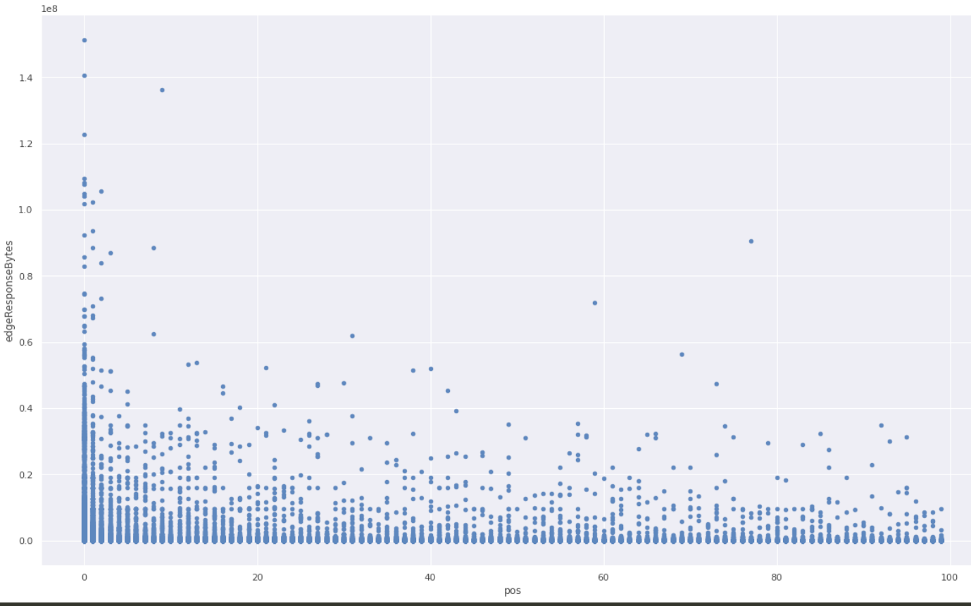
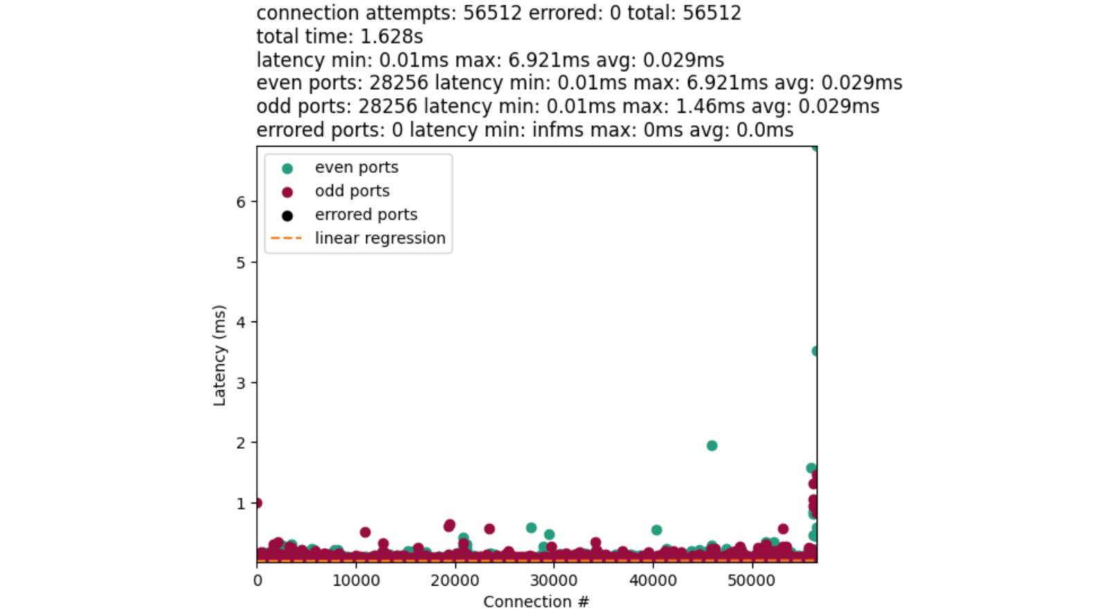
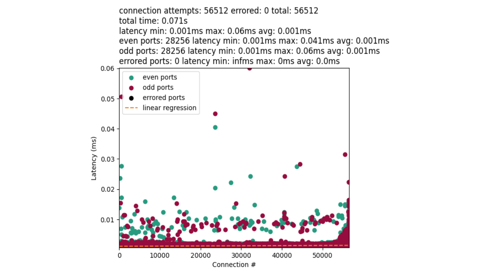
Here’s a graph showing how the lookup throughput for LPM tries (measured in million ops/sec) degrades as the number of entries increases, from 1 entry up to 100K entries.
Once you reach 1 million entries, throughput is around 1.5 million ops/sec, and continues to fall as the number of entries increases.
Why is this? Initially, this is because of the L1 dcache miss rate. All of those nodes that need to be traversed in the trie are potential cache miss opportunities.
As you can see from the graph, L1 dcache miss rate remains relatively steady and yet the throughput continues to decline. At around 80K entries, dTLB miss rate becomes the bottleneck.
Because BPF LPM tries to dynamically allocate individual nodes from a freelist of kernel memory, these nodes can live at arbitrary addresses. Which means traversing a path through a trie almost certainly will incur cache misses and potentially dTLB misses. This gets worse as the number of entries, and height of the trie, increases.
Where do we go from here?
By understanding the current limitations of the BPF LPM trie, we can now work towards building a more performant and efficient solution for the future of the Internet.
We’ve already contributed these benchmarks to the upstream Linux kernel — but that’s only the start. We have plans to improve the performance of BPM LPM tries, particularly the lookup function which is heavily used for our workloads. This post covered a number of optimisations that are already used by the net/ipv4/fib_trie.c code, so a natural first step is to refactor that code so that a common Level Compressed trie implementation can be used. Expect future blog posts to explore this work in depth.
The web is the most powerful application platform in existence. As long as you have the right API, you can safely run anything you want in a browser.
Well… anything but cryptography.
It is as true today as it was in 2011 that Javascript cryptography is Considered Harmful. The main problem is code distribution. Consider an end-to-end-encrypted messaging web application. The application generates cryptographic keys in the client’s browser that lets users view and send end-to-end encrypted messages to each other. If the application is compromised, what would stop the malicious actor from simply modifying their Javascript to exfiltrate messages?
It is interesting to note that smartphone apps don’t have this issue. This is because app stores do a lot of heavy lifting to provide security for the app ecosystem. Specifically, they provide integrity, ensuring that apps being delivered are not tampered with, consistency, ensuring all users get the same app, and transparency, ensuring that the record of versions of an app is truthful and publicly visible.
It would be nice if we could get these properties for our end-to-end encrypted web application, and the web as a whole, without requiring a single central authority like an app store. Further, such a system would benefit all in-browser uses of cryptography, not just end-to-end-encrypted apps. For example, many web-based confidential LLMs, cryptocurrency wallets, and voting systems use in-browser Javascript cryptography for the last step of their verification chains.
In this post, we will provide an early look at such a system, called Web Application Integrity, Consistency, and Transparency (WAICT) that we have helped author. WAICT is a W3C-backed effort among browser vendors, cloud providers, and encrypted communication developers to bring stronger security guarantees to the entire web. We will discuss the problem we need to solve, and build up to a solution resembling the current transparency specification draft. We hope to build even wider consensus on the solution design in the near future.
Defining the Web Application
In order to talk about security guarantees of a web application, it is first necessary to define precisely what the application is. A smartphone application is essentially just a zip file. But a website is made up of interlinked assets, including HTML, Javascript, WASM, and CSS, that can each be locally or externally hosted. Further, if any asset changes, it could drastically change the functioning of the application. A coherent definition of an application thus requires the application to commit to precisely the assets it loads. This is done using integrity features, which we describe now.
Subresource Integrity
An important building block for defining a single coherent application is subresource integrity (SRI). SRI is a feature built into most browsers that permits a website to specify the cryptographic hash of external resources, e.g.,
This causes the browser to fetch underscore.js from cdnjs.cloudflare.com and verify that its SHA-512 hash matches the given hash in the tag. If they match, the script is loaded. If not, an error is thrown and nothing is executed.
If every external script, stylesheet, etc. on a page comes with an SRI integrity attribute, then the whole page is defined by just its HTML. This is close to what we want, but a web application can consist of many pages, and there is no way for a page to enforce the hash of the pages it links to.
Integrity Manifest
We would like to have a way of enforcing integrity on an entire site, i.e., every asset under a domain. For this, WAICT defines an integrity manifest, a configuration file that websites can provide to clients. One important item in the manifest is the asset hashes dictionary, mapping a hash belonging to an asset that the browser might load from that domain, to the path of that asset. Assets that may occur at any path, e.g., an error page, map to the empty string:
The other main component of the manifest is the integrity policy, which tells the browser which data types are being enforced and how strictly. For example, the policy in the manifest below will:
Reject any script before running it, if it’s missing an SRI tag and doesn’t appear in the hashes
Reject any WASM possibly after running it, if it’s missing an SRI tag and doesn’t appear in hashes
Thus, when both SRI and integrity manifests are used, the entire site and its interpretation by the browser is uniquely determined by the hash of the integrity manifest. This is exactly what we wanted. We have distilled the problem of endowing authenticity, consistent distribution, etc. to a web application to one of endowing the same properties to a single hash.
Achieving Transparency
Recall, a transparent web application is one whose code is stored in a publicly accessible, append-only log. This is helpful in two ways: 1) if a user is served malicious code and they learn about it, there is a public record of the code they ran, and so they can prove it to external parties, and 2) if a user is served malicious code and they don’t learn about it, there is still a chance that an external auditor may comb through the historical web application code and find the malicious code anyway. Of course, transparency does not help detect malicious code or even prevent its distribution, but it at least makes it publicly auditable.
Now that we have a single hash that commits to an entire website’s contents, we can talk about ensuring that that hash ends up in a public log. We have several important requirements here:
Do not break existing sites. This one is a given. Whatever system gets deployed, it should not interfere with the correct functioning of existing websites. Participation in transparency should be strictly opt-in.
No added round trips. Transparency should not cause extra network round trips between the client and the server. Otherwise there will be a network latency penalty for users who want transparency.
User privacy. A user should not have to identify themselves to any party more than they already do. That means no connections to new third parties, and no sending identifying information to the website.
User statelessness. A user should not have to store site-specific data. We do not want solutions that rely on storing or gossipping per-site cryptographic information.
Non-centralization. There should not be a single point of failure in the system—if any single party experiences downtime, the system should still be able to make progress. Similarly, there should be no single point of trust—if a user distrusts any single party, the user should still receive all the security benefits of the system.
Ease of opt-in. The barrier of entry for transparency should be as low as possible. A site operator should be able to start logging their site cheaply and without being an expert.
Ease of opt-out. It should be easy for a website to stop participating in transparency. Further, to avoid accidental lock-in like the defunct HPKP spec, it should be possible for this to happen even if all cryptographic material is lost, e.g., in the seizure or selling of a domain.
Opt-out is transparent. As described before, because transparency is optional, it is possible for an attacker to disable the site’s transparency, serve malicious content, then enable transparency again. We must make sure this kind of attack is detectable, i.e., the act of disabling transparency must itself be logged somewhere.
Monitorability. A website operator should be able to efficiently monitor the transparency information being published about their website. In particular, they should not have to run a high-network-load, always-on program just to notify them if their site has been hijacked.
With these requirements in place, we can move on to construction. We introduce a data structure that will be essential to the design.
Hash Chain
Almost everything in transparency is an append-only log, i.e., a data structure that acts like a list and has the ability to produce an inclusion proof, i.e., a proof that an element occurs at a particular index in the list; and a consistency proof, i.e., a proof that a list is an extension of a previous version of the list. A consistency proof between two lists demonstrates that no elements were modified or deleted, only added.
The simplest possible append-only log is a hash chain, a list-like data structure wherein each subsequent element is hashed into the running chain hash. The final chain hash is a succinct representation of the entire list.
A hash chain. The green nodes represent the chain hash, i.e., the hash of the element below it, concatenated with the previous chain hash.
The proof structures are quite simple. To prove inclusion of the element at index i, the prover provides the chain hash before i, and all the elements after i:
Proof of inclusion for the second element in the hash chain. The verifier knows only the final chain hash. It checks equality of the final computed chain hash with the known final chain hash. The light green nodes represent hashes that the verifier computes.
Similarly, to prove consistency between the chains of size i and j, the prover provides the elements between i and j:
Proof of consistency of the chain of size one and chain of size three. The verifier has the chain hashes from the starting and ending chains. It checks equality of the final computed chain hash with the known ending chain hash. The light green nodes represent hashes that the verifier computes.
Building Transparency
We can use hash chains to build a transparency scheme for websites.
Per-Site Logs
As a first step, let’s give every site its own log, instantiated as a hash chain (we will discuss how these all come together into one big log later). The items of the log are just the manifest of the site at a particular point in time:
A site’s hash chain-based log, containing three historical manifests.
In reality, the log does not store the manifest itself, but the manifest hash. Sites designate an asset host that knows how to map hashes to the data they reference. This is a content-addressable storage backend, and can be implemented using strongly cached static hosting solutions.
A log on its own is not very trustworthy. Whoever runs the log can add and remove elements at will and then recompute the hash chain. To maintain the append-only-ness of the chain, we designate a trusted third party, called a witness. Given a hash chain consistency proof and a new chain hash, a witness:
Verifies the consistency proof with respect to its old stored chain hash, and the new provided chain hash.
If successful, signs the new chain hash along with a signature timestamp.
Now, when a user navigates to a website with transparency enabled, the sequence of events is:
The site serves its manifest, an inclusion proof showing that the manifest appears in the log, and all the signatures from all the witnesses who have validated the log chain hash.
The browser verifies the signatures from whichever witnesses it trusts.
The browser verifies the inclusion proof. The manifest must be the newest entry in the chain (we discuss how to serve old manifests later).
The browser proceeds with the usual manifest and SRI integrity checks.
At this point, the user knows that the given manifest has been recorded in a log whose chain hash has been saved by a trustworthy witness, so they can be reasonably sure that the manifest won’t be removed from history. Further, assuming the asset host functions correctly, the user knows that a copy of all the received code is readily available.
The need to signal transparency. The above algorithm works, but we have a problem: if an attacker takes control of a site, they can simply stop serving transparency information and thus implicitly disable transparency without detection. So we need an explicit mechanism that keeps track of every website that has enrolled into transparency.
The Transparency Service
To store all the sites enrolled into transparency, we want a global data structure that maps a site domain to the site log’s chain hash. One efficient way of representing this is a prefix tree (a.k.a., a trie). Every leaf in the tree corresponds to a site’s domain, and its value is the chain hash of that site’s log, the current log size, and the site’s asset host URL. For a site to prove validity of its transparency data, it will have to present an inclusion proof for its leaf. Fortunately, these proofs are efficient for prefix trees.
A prefix tree with four elements. Each leaf’s path corresponds to a domain. Each leaf’s value is the chain hash of its site’s log.
To add itself to the tree, a site proves possession of its domain to the transparency service, i.e., the party that operates the prefix tree, and provides an asset host URL. To update the entry, the site sends the new entry to the transparency service, which will compute the new chain hash. And to unenroll from transparency, the site just requests to have its entry removed from the tree (an adversary can do this too; we discuss how to detect this below).
Proving to Witnesses and Browsers
Now witnesses only need to look at the prefix tree instead of individual site logs, and thus they must verify whole-tree updates. The most important thing to ensure is that every site’s log is append-only. So whenever the tree is updated, it must produce a “proof” containing every new/deleted/modified entry, as well as a consistency proof for each entry showing that the site log corresponding to that entry has been properly appended to. Once the witness has verified this prefix tree update proof, it signs the root.
The sequence of updating a site’s assets and serving the site with transparency enabled.
The client-side verification procedure is as in the previous section, with two modifications:
The client now verifies two inclusion proofs: one for the integrity policy’s membership in the site log, and one for the site log’s membership in a prefix tree.
The client verifies the signature over the prefix tree root, since the witness no longer signs individual chain hashes. As before, the acceptable public keys are whichever witnesses the client trusts.
Signaling transparency. Now that there is a single source of truth, namely the prefix tree, a client can know a site is enrolled in transparency by simply fetching the site’s entry in the tree. This alone would work, but it violates our requirement of “no added round trips,” so we instead require that client browsers will ship with the list of sites included in the prefix tree. We call this the transparency preload list.
If a site appears in the preload list, the browser will expect it to provide an inclusion proof in the prefix tree, or else a proof of non-inclusion in a newer version of the prefix tree, thereby showing they’ve unenrolled. The site must provide one of these proofs until the last preload list it appears in has expired. Finally, even though the preload list is derived from the prefix tree, there is nothing enforcing this relationship. Thus, the preload list should also be published transparently.
Filling in Missing Properties
Remember we still have the requirements of monitorability, opt-out being transparent, and no single point of failure/trust. We fill in those details now.
Adding monitorability. So far, in order for a site operator to ensure their site was not hijacked, they would have to constantly query every transparency service for its domain and verify that it hasn’t been tampered with. This is certainly better than the 500k events per hour that CT monitors have to ingest, but it still requires the monitor to be constantly polling the prefix tree, and it imposes a constant load for the transparency service.
We add a field to the prefix tree leaf structure: the leaf now stores a “created” timestamp, containing the time the leaf was created. Witnesses ensure that the “created” field remains the same over all leaf updates (and it is deleted when the leaf is deleted). To monitor, a site operator need only keep the last observed “created” and “log size” fields of its leaf. If it fetches the latest leaf and sees both unchanged, it knows that no changes occurred since the last check.
Adding transparency of opt-out. We must also do the same thing as above for leaf deletions. When a leaf is deleted, a monitor should be able to learn when the deletion occurred within some reasonable time frame. Thus, rather than outright removing a leaf, the transparency service responds to unenrollment requests by replacing the leaf with a tombstone value, containing just a “created” timestamp. As before, witnesses ensure that this field remains unchanged until the leaf is permanently deleted (after some visibility period) or re-enrolled.
Permitting multiple transparency services. Since we require that there be no single point of failure or trust, we imagine an ecosystem where there are a handful of non-colluding, reasonably trustworthy transparency service providers, each with their own prefix tree. Like Certificate Transparency (CT), this set should not be too large. It must be small enough that reasonable levels of trust can be established, and so that independent auditors can reasonably handle the load of verifying all of them.
Ok that’s the end of the most technical part of this post. We’re now going to talk about how to tweak this system to provide all kinds of additional nice properties.
(Not) Achieving Consistency
Transparency would be useless if, every time a site updates, it serves 100,000 new versions of itself. Any auditor would have to go through every single version of the code in order to ensure no user was targeted with malware. This is bad even if the velocity of versions is lower. If a site publishes just one new version per week, but every version from the past ten years is still servable, then users can still be served extremely old, potentially vulnerable versions of the site, without anyone knowing. Thus, in order to make transparency valuable, we need consistency, the property that every browser sees the same version of the site at a given time.
We will not achieve the strongest version of consistency, but it turns out that weaker notions are sufficient for us. If, unlike the above scenario, a site had 8 valid versions of itself at a given time, then that would be pretty manageable for an auditor. So even though it’s true that users don’t all see the same version of the site, they will all still benefit from transparency, as desired.
We describe two types of inconsistency and how we mitigate them.
Tree Inconsistency
Tree inconsistency occurs when transparency services’ prefix trees disagree on the chain hash of a site, thus disagreeing on the history of the site. One way to fully eliminate this is to establish a consensus mechanism for prefix trees. A simple one is majority voting: if there are five transparency services, a site must present three tree inclusion proofs to a user, showing the chain hash is present in three trees. This, of course, triples the tree inclusion proof size, and lowers the fault tolerance of the entire system (if three log operators go down, then no transparent site can publish any updates).
Instead of consensus, we opt to simply limit the amount of inconsistency by limiting the number of transparency services. In 2025, Chrome trusts eight Certificate Transparency logs. A similar number of transparency services would be fine for our system. Plus, it is still possible to detect and prove the existence of inconsistencies between trees, since roots are signed by witnesses. So if it becomes the norm to use the same version on all trees, then social pressure can be applied when sites violate this.
Temporal Inconsistency
Temporal inconsistency occurs when a user gets a newer or older version of the site (both still unexpired), depending on some external factors such as geographic location or cookie values. In the extreme, as stated above, if a signed prefix root is valid for ten years, then a site can serve a user any version of the site from the last ten years.
As with tree inconsistency, this can be resolved using consensus mechanisms. If, for example, the latest manifest were published on a blockchain, then a user could fetch the latest blockchain head and ensure they got the latest version of the site. However, this incurs an extra network round trip for the client, and requires sites to wait for their hash to get published on-chain before they can update. More importantly, building this kind of consensus mechanism into our specification would drastically increase its complexity. We’re aiming for v1.0 here.
We mitigate temporal inconsistency by requiring reasonably short validity periods for witness signatures. Making prefix root signatures valid for, e.g., one week would drastically limit the number of simultaneously servable versions. The cost is that site operators must now query the transparency service at least once a week for the new signed root and inclusion proof, even if nothing in the site changed. The sites cannot skip this, and the transparency service must be able to handle this load. This parameter must be tuned carefully.
Beyond Integrity, Consistency, and Transparency
Providing integrity, consistency, and transparency is already a huge endeavor, but there are some additional app store-like security features that can be integrated into this system without too much work.
Code Signing
One problem that WAICT doesn’t solve is that of provenance: where did the code the user is running come from, precisely? In settings where audits of code happen frequently, this is not so important, because some third party will be reading the code regardless. But for smaller self-hosted deployments of open-source software, this may not be viable. For example, if Alice hosts her own version of Cryptpad for her friend Bob, how can Bob be sure the code matches the real code in Cryptpad’s Github repo?
WEBCAT. The folks at the Freedom of Press Foundation (FPF) have built a solution to this, called WEBCAT. This protocol allows site owners to announce the identities of the developers that have signed the site’s integrity manifest, i.e., have signed all the code and other assets that the site is serving to the user. Users with the WEBCAT plugin can then see the developer’s Sigstore signatures, and trust the code based on that.
We’ve made WAICT extensible enough to fit WEBCAT inside and benefit from the transparency components. Concretely, we permit manifests to hold additional metadata, which we call extensions. In this case, the extension holds a list of developers’ Sigstore identities. To be useful, browsers must expose an API for browser plugins to access these extension values. With this API, independent parties can build plugins for whatever feature they wish to layer on top of WAICT.
Cooldown
So far we have not built anything that can prevent attacks in the moment. An attacker who breaks into a website can still delete any code-signing extensions, or just unenroll the site from transparency entirely, and continue with their attack as normal. The unenrollment will be logged, but the malicious code will not be, and by the time anyone sees the unenrollment, it may be too late.
To prevent spontaneous unenrollment, we can enforce unenrollment cooldown client-side. Suppose the cooldown period is 24 hours. Then the rule is: if a site appears on the preload list, then the client will require that either 1) the site have transparency enabled, or 2) the site have a tombstone entry that is at least 24 hours old. Thus, an attacker will be forced to either serve a transparency-enabled version of the site, or serve a broken site for 24 hours.
Similarly, to prevent spontaneous extension modifications, we can enforce extension cooldown on the client. We will take code signing as an example, saying that any change in developer identities requires a 24 hour waiting period to be accepted. First, we require that extension dev-ids has a preload list of its own, letting the client know which sites have opted into code signing (if a preload list doesn’t exist then any site can delete the extension at any time). The client rule is as follows: if the site appears in the preload list, then both 1) dev-ids must exist as an extension in the manifest, and 2) dev-ids-inclusion must contain an inclusion proof showing that the current value of dev-ids was in a prefix tree that is at least 24 hours old. With this rule, a client will reject values of dev-ids that are newer than a day. If a site wants to delete dev-ids, they must 1) request that it be removed from the preload list, and 2) in the meantime, replace the dev-ids value with the empty string and update dev-ids-inclusion to reflect the new value.
Deployment Considerations
There are a lot of distinct roles in this ecosystem. Let’s sketch out the trust and resource requirements for each role.
Transparency service. These parties store metadata for every transparency-enabled site on the web. If there are 100 million domains, and each entry is 256B each (a few hashes, plus a URL), this comes out to 26GB for a single tree, not including the intermediate hashes. To prevent size blowup, there would probably have to be a pruning rule that unenrolls sites after a long inactivity period. Transparency services should have largely uncorrelated downtime, since, if all services go down, no transparency-enabled site can make any updates. Thus, transparency services must have a moderate amount of storage, be relatively highly available, and have downtime periods uncorrelated with each other.
Transparency services require some trust, but their behavior is narrowly constrained by witnesses. Theoretically, a service can replace any leaf’s chain hash with its own, and the witness will validate it (as long as the consistency proof is valid). But such changes are detectable by anyone that monitors that leaf.
Witness. These parties verify prefix tree updates and sign the resulting roots. Their storage costs are similar to that of a transparency service, since they must keep a full copy of a prefix tree for every transparency service they witness. Also like the transparency services, they must have high uptime. Witnesses must also be trusted to keep their signing key secret for a long period of time, at least long enough to permit browser trust stores to be updated when a new key is created.
Asset host. These parties carry little trust. They cannot serve bad data, since any query response is hashed and compared to a known hash. The only malicious behavior an asset host can do is refuse to respond to queries. Asset hosts can also do this by accident due to downtime.
Client. This is the most trust-sensitive part. The client is the software that performs all the transparency and integrity checks. This is, of course, the web browser itself. We must trust this.
We at Cloudflare would like to contribute what we can to this ecosystem. It should be possible to run both a transparency service and a witness. Of course, our witness should not monitor our own transparency service. Rather, we can witness other organizations’ transparency services, and our transparency service can be witnessed by other organizations.
Supporting Alternate Ecosystems
WAICT should be compatible with non-standard ecosystems, ones where the large players do not really exist, or at least not in the way they usually do. We are working with the FPF on defining transparency for alternate ecosystems with different network and trust environments. The primary example we have is that of the Tor ecosystem.
A paranoid Tor user may not trust existing transparency services or witnesses, and there might not be any other trusted party with the resources to self-host these functionalities. For this use case, it may be reasonable to put the prefix tree on a blockchain somewhere. This makes the usual domain validation impossible (there’s no validator server to speak of), but this is fine for onion services. Since an onion address is just a public key, a signature is sufficient to prove ownership of the domain.
One consequence of a consensus-backed prefix tree is that witnesses are now unnecessary, and there is only need for the single, canonical, transparency service. This mostly solves the problems of tree inconsistency at the expense of latency of updates.
Next Steps
We are still very early in the standardization process. One of the more immediate next steps is to get subresource integrity working for more data types, particularly WASM and images. After that, we can begin standardizing the integrity manifest format. And then after that we can start standardizing all the other features. We intend to work on this specification hand-in-hand with browsers and the IETF, and we hope to have some exciting betas soon.
In the meantime, you can follow along with our transparency specification draft, check out the open problems, and share your ideas. Pull requests and issues are always welcome!
Acknowledgements
Many thanks to Dennis Jackson from Mozilla for the lengthy back-and-forth meetings on design, to Giulio B and Cory Myers from FPF for their immensely helpful influence and feedback, and to Richard Hansen for great feedback.
Every second, 84 million HTTP requests are hitting Cloudflare across our fleet of data centers in 330 cities. It means that even the rarest of bugs can show up frequently. In fact, it was our scale that recently led us to discover a bug in Go’s arm64 compiler which causes a race condition in the generated code.
This post breaks down how we first encountered the bug, investigated it, and ultimately drove to the root cause.
Investigating a strange panic
We run a service in our network which configures the kernel to handle traffic for some products like Magic Transit and Magic WAN. Our monitoring watches this closely, and it started to observe very sporadic panics on arm64 machines.
We first saw one with a fatal error stating that traceback did not unwind completely. That error suggests that invariants were violated when traversing the stack, likely because of stack corruption. After a brief investigation we decided that it was probably rare stack memory corruption. This was a largely idle control plane service where unplanned restarts have negligible impact, and so we felt that following up was not a priority unless it kept happening.
And then it kept happening.
Coredumps per hour
When we first saw this bug we saw that the fatal errors correlated with recovered panics. These were caused by some old code which used panic/recover as error handling.
At this point, our theory was:
All of the fatal panics happen within stack unwinding.
We correlated an increased volume of recovered panics with these fatal panics.
Recovering a panic unwinds goroutine stacks to call deferred functions.
A related Go issue (#73259) reported an arm64 stack unwinding crash.
Let’s stop using panic/recover for error handling and wait out the upstream fix?
So we did that and watched as fatal panics stopped occurring as the release rolled out. Fatal panics gone, our theoretical mitigation seemed to work, and this was no longer our problem. We subscribed to the upstream issue so we could update when it was resolved and put it out of our minds.
But, this turned out to be a much stranger bug than expected. Putting it out of our minds was premature as the same class of fatal panics came back at a much higher rate. A month later, we were seeing up to 30 daily fatal panics with no real discernible cause; while that might account for only one machine a day in less than 10% of our data centers, we found it concerning that we didn’t understand the cause. The first thing we checked was the number of recovered panics, to match our previous pattern, but there were none. More interestingly, we could not correlate this increased rate of fatal panics with anything. A release? Infrastructure changes? The position of Mars?
At this point we felt like we needed to dive deeper to better understand the root cause. Pattern matching and hoping was clearly insufficient.
We saw two classes of this bug — a crash while accessing invalid memory and an explicitly checked fatal error.
Now we could observe some clear patterns. Both errors occur when unwinding the stack in (*unwinder).next. In one case we saw an intentionalfatal error as the runtime identified that unwinding could not complete and the stack was in a bad state. In the other case there was a direct memory access error that happened while trying to unwind the stack. The segfault was discussed in the GitHub issue and a Go engineer identified it as dereference of a go scheduler struct, m, whenunwinding.
A review of Go scheduler structs
Go uses a lightweight userspace scheduler to manage concurrency. Many goroutines are scheduled on a smaller number of kernel threads – this is often referred to as M:N scheduling. Any individual goroutine can be scheduled on any kernel thread. The scheduler has three core types – g (the goroutine), m (the kernel thread, or “machine”), and p (the physical execution context, or “processor”). For a goroutine to be scheduled a free m must acquire a free p, which will execute a g. Each g contains a field for its m if it is currently running, otherwise it will be nil. This is all the context needed for this post but the go runtime docs explore this more comprehensively.
At this point we can start to make inferences on what’s happening: the program crashes because we try to unwind a goroutine stack which is invalid. In the first backtrace, if a return address is null, we call finishInternal and abort because the stack was not fully unwound. The segmentation fault case in the second backtrace is a bit more interesting: if instead the return address is non-zero but not a function then the unwinder code assumes that the goroutine is currently running. It’ll then dereference m and fault by accessing m.incgo (the offset of incgo into struct m is 0x118, the faulting memory access).
What, then, is causing this corruption? The traces were difficult to get anything useful from – our service has hundreds if not thousands of active goroutines. It was fairly clear from the beginning that the panic was remote from the actual bug. The crashes were all observed while unwinding the stack and if this were an issue any time the stack was unwound on arm64 we would be seeing it in many more services. We felt pretty confident that the stack unwinding was happening correctly but on an invalid stack.
Our investigation stalled for a while at this point – making guesses, testing guesses, trying to infer if the panic rate went up or down, or if nothing changed. There was a known issue on Go’s GitHub issue tracker which matched our symptoms almost exactly, but what they discussed was mostly what we already knew. At some point when looking through the linked stack traces we realized that their crash referenced an old version of a library that we were also using – Go Netlink.
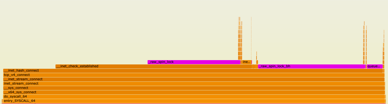
We spot-checked a few stack traces and confirmed the presence of this Netlink library. Querying our logs showed that not only did we share a library – every single segmentation fault we observed had happened while preemptingNetlinkSocket.Receive.
What’s (async) preemption?
In the prehistoric era of Go (<=1.13) the runtime was cooperatively scheduled. A goroutine would run until it decided it was ready to yield to the scheduler – usually due to explicit calls to runtime.Gosched() or injected yield points at function calls/IO operations. SinceGo 1.14 the runtime instead does async preemption. The Go runtime has a thread sysmon which tracks the runtime of goroutines and will preempt any that run for longer than 10ms (at time of writing). It does this by sending SIGURG to the OS thread and in the signal handler will modify the program counter and stack to mimic a call to asyncPreempt.
At this point we had two broad theories:
This is a Go Netlink bug – likely due to unsafe.Pointer usage which invoked undefined behavior but is only actually broken on arm64
This is a Go runtime bug and we’re only triggering it in NetlinkSocket.Receive for some reason
After finding the same bug publicly reported upstream, we were feeling confident this was caused by a Go runtime bug. However, upon seeing that both issues implicated the same function, we felt more skeptical – notably the Go Netlink library uses unsafe.Pointer so memory corruption was a plausible explanation even if we didn’t understand why.
After an unsuccessful code audit we had hit a wall. The crashes were rare and remote from the root cause. Maybe these crashes were caused by a runtime bug, maybe they were caused by a Go Netlink bug. It seemed clear that there was something wrong with this area of the code, but code auditing wasn’t going anywhere.
Breakthrough
At this point we had a fairly good understanding of what was crashing but very little understanding of why it was happening. It was clear that the root cause of the stack unwinder crashing was remote from the actual crash, and that it had to do with (*NetlinkSocket).Receive, but why? We were able to capture a coredump of a production crash and view it in a debugger. The backtrace confirmed what we already knew – that there was a segmentation fault when unwinding a stack. The crux of the issue revealed itself when we looked at the goroutine which had been preempted while calling (*NetlinkSocket).Receive.
(dlv) bt
0  0x0000555577579dec in runtime.asyncPreempt2
   at /usr/local/go/src/runtime/preempt.go:306
1  0x00005555775bc94c in runtime.asyncPreempt
   at /usr/local/go/src/runtime/preempt_arm64.s:47
2  0x0000555577cb2880 in github.com/vishvananda/netlink/nl.(*NetlinkSocket).Receive
   at
/vendor/github.com/vishvananda/netlink/nl/nl_linux.go:779
3  0x0000555577cb19a8 in github.com/vishvananda/netlink/nl.(*NetlinkRequest).Execute
   at
/vendor/github.com/vishvananda/netlink/nl/nl_linux.go:532
4  0x0000555577551124 in runtime.heapSetType
   at /usr/local/go/src/runtime/mbitmap.go:714
5  0x0000555577551124 in runtime.heapSetType
   at /usr/local/go/src/runtime/mbitmap.go:714
...
(dlv) disass -a 0x555577cb2878 0x555577cb2888
TEXT github.com/vishvananda/netlink/nl.(*NetlinkSocket).Receive(SB) /vendor/github.com/vishvananda/netlink/nl/nl_linux.go
        nl_linux.go:779 0x555577cb2878  fdfb7fa9        LDP -8(RSP), (R29, R30)
        nl_linux.go:779 0x555577cb287c  ff430191        ADD $80, RSP, RSP
        nl_linux.go:779 0x555577cb2880  ff434091        ADD $(16<<12), RSP, RSP
        nl_linux.go:779 0x555577cb2884  c0035fd6        RET
The goroutine was paused between two opcodes in the function epilogue. Since the process of unwinding a stack relies on the stack frame being in a consistent state, it felt immediately suspicious that we preempted in the middle of adjusting the stack pointer. The goroutine had been paused at 0x555577cb2880, between ADD $80, RSP, RSP and ADD $(16<<12), RSP, RSP.
We queried the service logs to confirm our theory. This wasn’t isolated – the majority of stack traces showed that this same opcode was preempted. This was no longer a weird production crash we couldn’t reproduce. A crash happened when the Go runtime preempted between these two stack pointer adjustments. We had our smoking gun.
Building a minimal reproducer
At this point we felt pretty confident that this was actually just a runtime bug and it should be reproducible in an isolated environment without any dependencies. The theory at this point was:
Stack unwinding is triggered by garbage collection
Async preemption between a split stack pointer adjustment causes a crash
What if we make a function which splits the adjustment and then call it in a loop?
package main

import (
	"runtime"
)

//go:noinline
func big_stack(val int) int {
	var big_buffer = make([]byte, 1 << 16)

	sum := 0
	// prevent the compiler from optimizing out the stack
	for i := 0; i < (1<<16); i++ {
		big_buffer[i] = byte(val)
	}
	for i := 0; i < (1<<16); i++ {
		sum ^= int(big_buffer[i])
	}
	return sum
}

func main() {
	go func() {
		for {
			runtime.GC()
		}
	}()
	for {
		_ = big_stack(1000)
	}
}
This function ends up with a stack frame slightly larger than can be represented in 16 bits, and so on arm64 the Go compiler will split the stack pointer adjustment into two opcodes. If the runtime preempts between these opcodes then the stack unwinder will read an invalid stack pointer and crash.
; epilogue for main.big_stack
ADD $8, RSP, R29
ADD $(16<<12), R29, R29
ADD $16, RSP, RSP
; preemption is problematic between these opcodes
ADD $(16<<12), RSP, RSP
RET
After running this for a few minutes the program panicked as expected!
A reproducible crash with standard library only? This felt like conclusive evidence that our problem was a runtime bug.
This was an extremely particular reproducer! Even now with a good understanding of the bug and its fix, some of the behavior is still puzzling. It’s a one-instruction race condition, so it’s unsurprising that small changes could have large impact. For example, this reproducer was originally written and tested on Go 1.23.4, but did not crash when compiled with 1.23.9 (the version in production), even though we could objdump the binary and see the split ADD still present! We don’t have a definite explanation for this behavior – even with the bug present there remain a few unknown variables which affect the likelihood of hitting the race condition.
A single-instruction race condition window
arm64 is a fixed-length 4-byte instruction set architecture. This has a lot of implications on codegen but most relevant to this bug is the fact that immediate length is limited.add gets a 12-bit immediate,mov gets a 16-bit immediate, etc. How does the architecture handle this when the operands don’t fit? It depends – ADD in particular reserves a bit for “shift left by 12” so any 24 bit addition can be decomposed into two opcodes. Other instructions are decomposed similarly, or just require loading an immediate into a register first.
The very last step of the Go compiler before emitting machine code involves transforming the program into obj.Prog structs. It’s a very low level intermediate representation (IR) that mostly serves to be translated into machine code.
Notably, this IR is not aware of immediate length limitations. Instead, this happens inasm7.go when Go’s internal intermediate representation is translated into arm64 machine code. The assembler will classify an immediate in conclass based on bit size and then use that when emitting instructions – extra if needed.
The Go assembler uses a combination of (mov, add) opcodes for some adds that fit in 16-bit immediates, and prefers (add, add + lsl 12) opcodes for 16-bit+ immediates.
In the larger stack case, there is a point between ADD x, RSP, RSP opcodes where the stack pointer is not pointing to the tip of a stack frame. We thought at first that this was a matter of memory corruption – that in handling async preemption the runtime would push a function call on the stack and corrupt the middle of the stack. However, this goroutine is already in the function epilogue – any data we corrupt is actively in the process of being thrown away. What’s the issue then?
The Go runtime often needs to unwind the stack, which means walking backwards through the chain of function calls. For example: garbage collection uses it to find live references on the stack, panicking relies on it to evaluate defer functions, and generating stack traces needs to print the call stack. For this to work the stack pointer must be accurate during unwinding because of how golang dereferences sp to determine the calling function. If the stack pointer is partially modified, the unwinder will look for the calling function in the middle of the stack. The underlying data is meaningless when interpreted as directions to a parent stack frame and then the runtime will likely crash.
When async preemption happens it will push a function call onto the stack but the parent stack frame is no longer correct because sp was only partially adjusted when the preemption happened. The crash flow looks something like this:
Async preemption happens between the two opcodes that add x, rsp expands to
The unwinder starts traversing the stack of the problematic goroutine and correctly unwinds up to the problematic function
The unwinder dereferences sp to determine the parent function
Almost certainly the data behind sp is not a function
Crash
We saw earlier a faulting stack trace which ended in (*NetlinkSocket).Receive – in this case stack unwinding faulted while it was trying to determine the parent frame.
Once we discovered the root cause we reported it with a reproducer and the bug was quickly fixed. This bug is fixed in go1.23.12, go1.24.6, and go1.25.0. Previously, the go compiler emitted a single add x, rsp instruction and relied on the assembler to split immediates into multiple opcodes as necessary. After this change, stacks larger than 1<<12 will build the offset in a temporary register and then add that to rsp in a single, indivisible opcode. A goroutine can be preempted before or after the stack pointer modification, but never during. This means that the stack pointer is always valid and there is no race condition.
This was a very fun problem to debug. We don’t often see bugs where you can accurately blame the compiler. Debugging it took weeks and we had to learn about areas of the Go runtime that people don’t usually need to think about. It’s a nice example of a rare race condition, the sort of bug that can only really be quantified at a large scale.
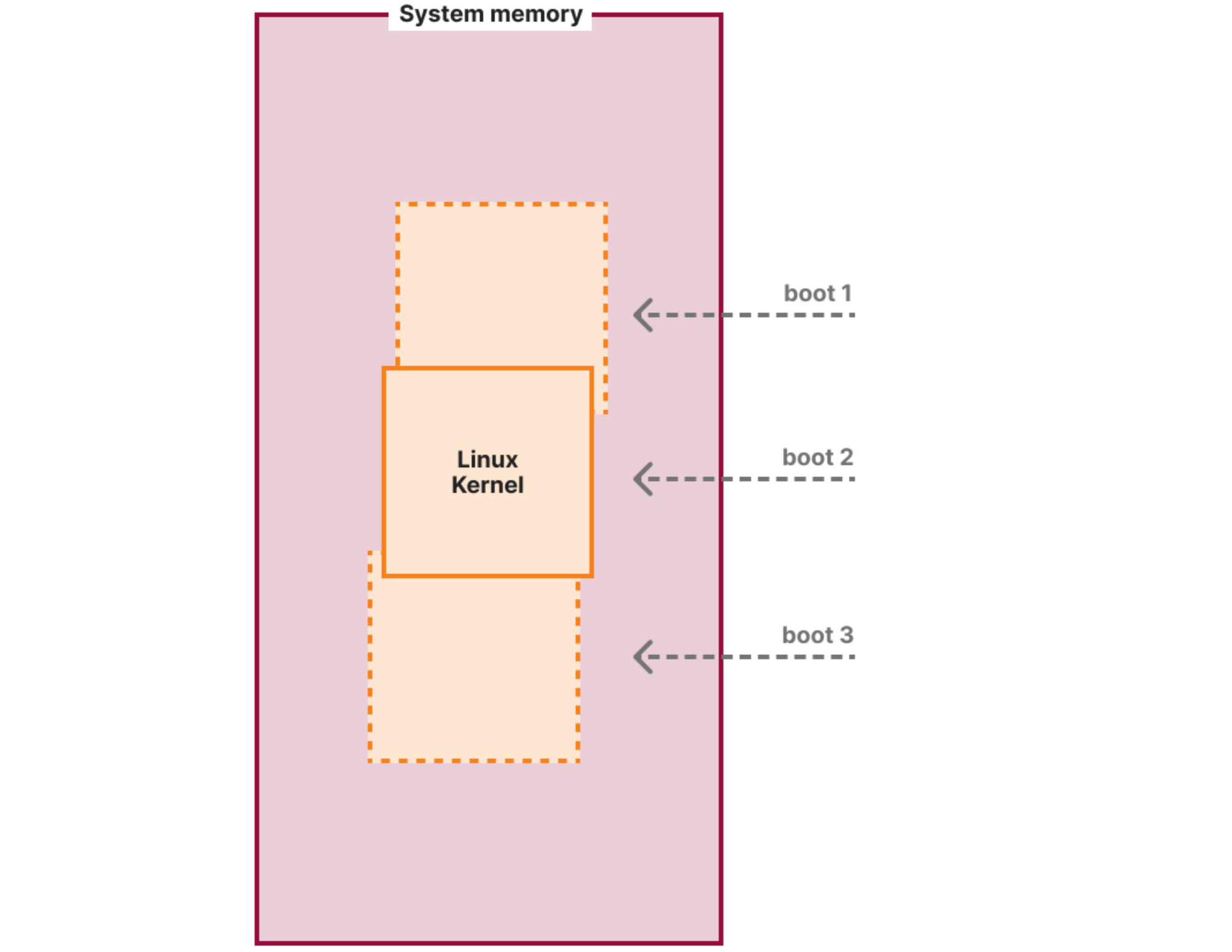
Building the fastest network requires work in many areas. We invest a lot of time in our hardware, to have efficient and fast machines. We invest in peering arrangements, to make sure we can talk to every part of the Internet with minimal delay. On top of this, we also have to invest in the software we run our network on, especially as each new product can otherwise add more processing delay.
No matter how fast messages arrive, we introduce a bottleneck if that software takes too long to think about how to process and respond to requests. Today we are excited to share a significant upgrade to our software that cuts the median time we take to respond by 10ms and delivers a 25% performance boost, as measured by third-party CDN performance tests.
We’ve spent the last year rebuilding major components of our system, and we’ve just slashed the latency of traffic passing through our network for millions of our customers. At the same time, we’ve made our system more secure, and we’ve reduced the time it takes for us to build and release new products.
Where did we start?
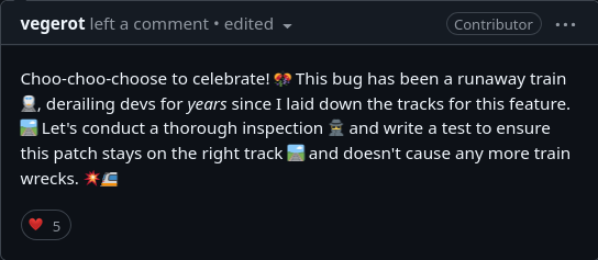
Every request that hits Cloudflare starts a journey through our network. It might come from a browser loading a webpage, a mobile app calling an API, or automated traffic from another service. These requests first terminate at our HTTP and TLS layer, then pass into a system we call FL, and finally through Pingora, which performs cache lookups or fetches data from the origin if needed.
FL is the brain of Cloudflare. Once a request reaches FL, we then run the various security and performance features in our network. It applies each customer’s unique configuration and settings, from enforcing WAF rules and DDoS protection to routing traffic to the Developer Platform and R2.
Built more than 15 years ago, FL has been at the core of Cloudflare’s network. It enables us to deliver a broad range of features, but over time that flexibility became a challenge. As we added more products, FL grew harder to maintain, slower to process requests, and more difficult to extend. Each new feature required careful checks across existing logic, and every addition introduced a little more latency, making it increasingly difficult to sustain the performance we wanted.
You can see how FL is key to our system — we’ve often called it the “brain” of Cloudflare. It’s also one of the oldest parts of our system: the first commit to the codebase was made by one of our founders, Lee Holloway, well before our initial launch. We’re celebrating our 15th Birthday this week – this system started 9 months before that!
commit 39c72e5edc1f05ae4c04929eda4e4d125f86c5ce
Author: Lee Holloway <q@t60.(none)>
Date:   Wed Jan 6 09:57:55 2010 -0800

    nginx-fl initial configuration
As the commit implies, the first version of FL was implemented based on the NGINX webserver, with product logic implemented in PHP. After 3 years, the system became too complex to manage effectively, and too slow to respond, and an almost complete rewrite of the running system was performed. This led to another significant commit, this time made by Dane Knecht, who is now our CTO.
From this point on, FL was implemented using NGINX, the OpenResty framework, and LuaJIT. While this was great for a long time, over the last few years it started to show its age. We had to spend increasing amounts of time fixing or working around obscure bugs in LuaJIT. The highly dynamic and unstructured nature of our Lua code, which was a blessing when first trying to implement logic quickly, became a source of errors and delay when trying to integrate large amounts of complex product logic. Each time a new product was introduced, we had to go through all the other existing products to check if they might be affected by the new logic.
It was clear that we needed a rethink. So, in July 2024, we cut an initial commit for a brand new, and radically different, implementation. To save time agreeing on a new name for this, we just called it “FL2”, and started, of course, referring to the original FL as “FL1”.
We weren’t starting from scratch. We’ve previously blogged about how we replaced another one of our legacy systems with Pingora, which is built in the Rust programming language, using the Tokio runtime. We’ve also blogged about Oxy, our internal framework for building proxies in Rust. We write a lot of Rust, and we’ve gotten pretty good at it.
We built FL2 in Rust, on Oxy, and built a strict module framework to structure all the logic in FL2.
Why Oxy?
When we set out to build FL2, we knew we weren’t just replacing an old system; we were rebuilding the foundations of Cloudflare. That meant we needed more than just a proxy; we needed a framework that could evolve with us, handle the immense scale of our network, and let teams move quickly without sacrificing safety or performance.
Oxy gives us a powerful combination of performance, safety, and flexibility. Built in Rust, it eliminates entire classes of bugs that plagued our Nginx/LuaJIT-based FL1, like memory safety issues and data races, while delivering C-level performance. At Cloudflare’s scale, those guarantees aren’t nice-to-haves, they’re essential. Every microsecond saved per request translates into tangible improvements in user experience, and every crash or edge case avoided keeps the Internet running smoothly. Rust’s strict compile-time guarantees also pair perfectly with FL2’s modular architecture, where we enforce clear contracts between product modules and their inputs and outputs.
But the choice wasn’t just about language. Oxy is the culmination of years of experience building high-performance proxies. It already powers several major Cloudflare services, from our Zero Trust Gateway to Apple’s iCloud Private Relay, so we knew it could handle the diverse traffic patterns and protocol combinations that FL2 would see. Its extensibility model lets us intercept, analyze, and manipulate traffic from layer 3 up to layer 7, and even decapsulate and reprocess traffic at different layers. That flexibility is key to FL2’s design because it means we can treat everything from HTTP to raw IP traffic consistently and evolve the platform to support new protocols and features without rewriting fundamental pieces.
Oxy also comes with a rich set of built-in capabilities that previously required large amounts of bespoke code. Things like monitoring, soft reloads, dynamic configuration loading and swapping are all part of the framework. That lets product teams focus on the unique business logic of their module rather than reinventing the plumbing every time. This solid foundation means we can make changes with confidence, ship them quickly, and trust they’ll behave as expected once deployed.
Smooth restarts – keeping the Internet flowing
One of the most impactful improvements Oxy brings is handling of restarts. Any software under continuous development and improvement will eventually need to be updated. In desktop software, this is easy: you close the program, install the update, and reopen it. On the web, things are much harder. Our software is in constant use and cannot simply stop. A dropped HTTP request can cause a page to fail to load, and a broken connection can kick you out of a video call. Reliability is not optional.
In FL1, upgrades meant restarts of the proxy process. Restarting a proxy meant terminating the process entirely, which immediately broke any active connections. That was particularly painful for long-lived connections such as WebSockets, streaming sessions, and real-time APIs. Even planned upgrades could cause user-visible interruptions, and unplanned restarts during incidents could be even worse.
Oxy changes that. It includes a built-in mechanism for graceful restarts that lets us roll out new versions without dropping connections whenever possible. When a new instance of an Oxy-based service starts up, the old one stops accepting new connections but continues to serve existing ones, allowing those sessions to continue uninterrupted until they end naturally.
This means that if you have an ongoing WebSocket session when we deploy a new version, that session can continue uninterrupted until it ends naturally, rather than being torn down by the restart. Across Cloudflare’s fleet, deployments are orchestrated over several hours, so the aggregate rollout is smooth and nearly invisible to end users.
We take this a step further by using systemd socket activation. Instead of letting each proxy manage its own sockets, we let systemd create and own them. This decouples the lifetime of sockets from the lifetime of the Oxy application itself. If an Oxy process restarts or crashes, the sockets remain open and ready to accept new connections, which will be served as soon as the new process is running. That eliminates the “connection refused” errors that could happen during restarts in FL1 and improves overall availability during upgrades.
We also built our own coordination mechanisms in Rust to replace Go libraries like tableflip with shellflip. This uses a restart coordination socket that validates configuration, spawns new instances, and ensures the new version is healthy before the old one shuts down. This improves feedback loops and lets our automation tools detect and react to failures immediately, rather than relying on blind signal-based restarts.
Composing FL2 from Modules
To avoid the problems we had in FL1, we wanted a design where all interactions between product logic were explicit and easy to understand.
So, on top of the foundations provided by Oxy, we built a platform which separates all the logic built for our products into well-defined modules. After some experimentation and research, we designed a module system which enforces some strict rules:
No IO (input or output) can be performed by the module.
The module provides a list of phases.
Phases are evaluated in a strictly defined order, which is the same for every request.
Each phase defines a set of inputs which the platform provides to it, and a set of outputs which it may emit.
Here’s an example of what a module phase definition looks like:
This phase is for our custom error page product. It takes a few things as input — information about the IP of the visitor, some header and other HTTP information, and some “module values.” Module values allow one module to pass information to another, and they’re key to making the strict properties of the module system workable. For example, this module needs some information that is produced by the output of our rulesets-based custom errors product (the “MODULE_VALUE_RULESETS_CUSTOM_ERRORS_OUTPUT” input). These input and output definitions are enforced at compile time.
While these rules are strict, we’ve found that we can implement all our product logic within this framework. The benefit of doing so is that we can immediately tell which other products might affect each other.
How to replace a running system
Building a framework is one thing. Building all the product logic and getting it right, so that customers don’t notice anything other than a performance improvement, is another.
The FL code base supports 15 years of Cloudflare products, and it’s changing all the time. We couldn’t stop development. So, one of our first tasks was to find ways to make the migration easier and safer.
Step 1 – Rust modules in OpenResty
It’s a big enough distraction from shipping products to customers to rebuild product logic in Rust. Asking all our teams to maintain two versions of their product logic, and reimplement every change a second time until we finished our migration was too much.
So, we implemented a layer in our old NGINX and OpenResty based FL which allowed the new modules to be run. Instead of maintaining a parallel implementation, teams could implement their logic in Rust, and replace their old Lua logic with that, without waiting for the full replacement of the old system.
For example, here’s part of the implementation for the custom error page module phase defined earlier (we’ve cut out some of the more boring details, so this doesn’t quite compile as-written):
pub(crate) fn callback(_services: &mut Services, input: &Input<'_>) -> Output {
    // Rulesets produced a response to serve - this can either come from a special
    // Cloudflare worker for serving custom errors, or be directly embedded in the rule.
    if let Some(rulesets_params) = input
        .get_module_value(MODULE_VALUE_RULESETS_CUSTOM_ERRORS_OUTPUT)
        .cloned()
    {
        // Select either the result from the special worker, or the parameters embedded
        // in the rule.
        let body = input
            .get_module_value(MODULE_VALUE_CUSTOM_ERRORS_FETCH_WORKER_RESPONSE)
            .and_then(|response| {
                handle_custom_errors_fetch_response("rulesets", response.to_owned())
            })
            .or(rulesets_params.body);

        // If we were able to load a body, serve it, otherwise let the next bit of logic
        // handle the response
        if let Some(body) = body {
            let final_body = replace_custom_error_tokens(input, &body);

            // Increment a metric recording number of custom error pages served
            custom_pages::pages_served("rulesets").inc();

            // Return a phase output with one final action, causing an HTTP response to be served.
            return Output::from(TerminalAction::ServeResponse(ResponseAction::OriginError {
                rulesets_params.status,
                source: "rulesets http_custom_errors",
                headers: rulesets_params.headers,
                body: Some(Bytes::from(final_body)),
            }));
        }
    }
}
The internal logic in each module is quite cleanly separated from the handling of data, with very clear and explicit error handling encouraged by the design of the Rust language.
Many of our most actively developed modules were handled this way, allowing the teams to maintain their change velocity during our migration.
Step 2 – Testing and automated rollouts
It’s essential to have a seriously powerful test framework to cover such a migration. We built a system, internally named Flamingo, which allows us to run thousands of full end-to-end test requests concurrently against our production and pre-production systems. The same tests run against FL1 and FL2, giving us confidence that we’re not changing behaviours.
Whenever we deploy a change, that change is rolled out gradually across many stages, with increasing amounts of traffic. Each stage is automatically evaluated, and only passes when the full set of tests have been successfully run against it – as well as overall performance and resource usage metrics being within acceptable bounds. This system is fully automated, and pauses or rolls back changes if the tests fail.
The benefit is that we’re able to build and ship new product features in FL2 within 48 hours – where it would have taken weeks in FL1. In fact, at least one of the announcements this week involved such a change!
Step 3 – Fallbacks
Over 100 engineers have worked on FL2, and we have over 130 modules. And we’re not quite done yet. We’re still putting the final touches on the system, to make sure it replicates all the behaviours of FL1.
So how do we send traffic to FL2 without it being able to handle everything? If FL2 receives a request, or a piece of configuration for a request, that it doesn’t know how to handle, it gives up and does what we’ve called a fallback – it passes the whole thing over to FL1. It does this at the network level – it just passes the bytes on to FL1.
As well as making it possible for us to send traffic to FL2 without it being fully complete, this has another massive benefit. When we have implemented a piece of new functionality in FL2, but want to double check that it is working the same as in FL1, we can evaluate the functionality in FL2, and then trigger a fallback. We are able to compare the behaviour of the two systems, allowing us to get a high confidence that our implementation was correct.
Step 4 – Rollout
We started running customer traffic through FL2 early in 2025, and have been progressively increasing the amount of traffic served throughout the year. Essentially, we’ve been watching two graphs: one with the proportion of traffic routed to FL2 going up, and another with the proportion of traffic failing to be served by FL2 and falling back to FL1 going down.
We started this process by passing traffic for our free customers through the system. We were able to prove that the system worked correctly, and drive the fallback rates down for our major modules. Our Cloudflare Community MVPs acted as an early warning system, smoke testing and flagging when they suspected the new platform might be the cause of a new reported problem. Crucially their support allowed our team to investigate quickly, apply targeted fixes, or confirm the move to FL2 was not to blame.
We then advanced to our paying customers, gradually increasing the amount of customers using the system. We also worked closely with some of our largest customers, who wanted the performance benefits of FL2, and onboarded them early in exchange for lots of feedback on the system.
Right now, most of our customers are using FL2. We still have a few features to complete, and are not quite ready to onboard everyone, but our target is to turn off FL1 within a few more months.
Impact of FL2
As we described at the start of this post, FL2 is substantially faster than FL1. The biggest reason for this is simply that FL2 performs less work. You might have noticed in the module definition example a line
filters: vec![],
Every module is able to provide a set of filters, which control whether they run or not. This means that we don’t run logic for every product for every request — we can very easily select just the required set of modules. The incremental cost for each new product we develop has gone away.
Another huge reason for better performance is that FL2 is a single codebase, implemented in a performance focussed language. In comparison, FL1 was based on NGINX (which is written in C), combined with LuaJIT (Lua, and C interface layers), and also contained plenty of Rust modules. In FL1, we spent a lot of time and memory converting data from the representation needed by one language, to the representation needed by another.
As a result, our internal measures show that FL2 uses less than half the CPU of FL1, and much less than half the memory. That’s a huge bonus — we can spend the CPU on delivering more and more features for our customers!
How do we measure if we are getting better?
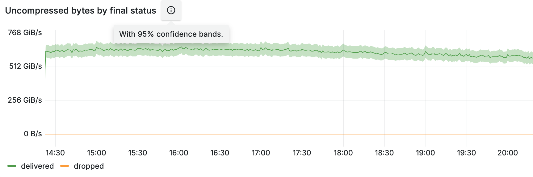
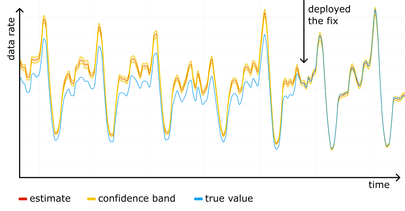
Using our own tools and independent benchmarks like CDNPerf, we measured the impact of FL2 as we rolled it out across the network. The results are clear: websites are responding 10 ms faster at the median, a 25% performance boost.
Security
FL2 is also more secure by design than FL1. No software system is perfect, but the Rust language brings us huge benefits over LuaJIT. Rust has strong compile-time memory checks and a type system that avoids large classes of errors. Combine that with our rigid module system, and we can make most changes with high confidence.
Of course, no system is secure if used badly. It’s easy to write code in Rust, which causes memory corruption. To reduce risk, we maintain strong compile time linting and checking, together with strict coding standards, testing and review processes.
We have long followed a policy that any unexplained crash of our systems needs to be investigated as a high priority. We won’t be relaxing that policy, though the main cause of novel crashes in FL2 so far has been due to hardware failure. The massively reduced rates of such crashes will give us time to do a good job of such investigations.
What’s next?
We’re spending the rest of 2025 completing the migration from FL1 to FL2, and will turn off FL1 in early 2026. We’re already seeing the benefits in terms of customer performance and speed of development, and we’re looking forward to giving these to all our customers.
We have one last service to completely migrate. The “HTTP & TLS Termination” box from the diagram way back at the top is also an NGINX service, and we’re midway through a rewrite in Rust. We’re making good progress on this migration, and expect to complete it early next year.
After that, when everything is modular, in Rust and tested and scaled, we can really start to optimize! We’ll reorganize and simplify how the modules connect to each other, expand support for non-HTTP traffic like RPC and streams, and much more.
If you’re interested in being part of this journey, check out our careers page for open roles – we’re always looking for new talent to help us to help build a better Internet.
How do you run SQL queries over petabytes of data… without a server?
We have an answer for that: R2 SQL, a serverless query engine that can sift through enormous datasets and return results in seconds.
This post details the architecture and techniques that make this possible. We’ll walk through our Query Planner, which uses R2 Data Catalog to prune terabytes of data before reading a single byte, and explain how we distribute the work across Cloudflare’s global network, Workers and R2 for massively parallel execution.
From catalog to query
During Developer Week 2025, we launched R2 Data Catalog, a managed Apache Iceberg catalog built directly into your Cloudflare R2 bucket. Iceberg is an open table format that provides critical database features like transactions and schema evolution for petabyte-scale object storage. It gives you a reliable catalog of your data, but it doesn’t provide a way to query it.
Until now, reading your R2 Data Catalog required setting up a separate service like Apache Spark or Trino. Operating these engines at scale is not easy: you need to provision clusters, manage resource usage, and be responsible for their availability, none of which contributes to the primary goal of getting value from your data.
R2 SQL removes that step entirely. It’s a serverless query engine that executes retrieval SQL queries against your Iceberg tables, right where your data lives.
Designing a query engine for petabytes
Object storage is fundamentally different from a traditional database’s storage. A database is structured by design; R2 is an ocean of objects, where a single logical table can be composed of potentially millions of individual files, large and small, with more arriving every second.
Apache Iceberg provides a powerful layer of logical organization on top of this reality. It works by managing the table’s state as an immutable series of snapshots, creating a reliable, structured view of the table by manipulating lightweight metadata files instead of rewriting the data files themselves.
However, this logical structure doesn’t change the underlying physical challenge: an efficient query engine must still find the specific data it needs within that vast collection of files, and this requires overcoming two major technical hurdles:
The I/O problem: A core challenge for query efficiency is minimizing the amount of data read from storage. A brute-force approach of reading every object is simply not viable. The primary goal is to read only the data that is absolutely necessary.
The Compute problem: The amount of data that does need to be read can still be enormous. We need a way to give the right amount of compute power to a query, which might be massive, for just a few seconds, and then scale it down to zero instantly to avoid waste.
Our architecture for R2 SQL is designed to solve these two problems with a two-phase approach: a Query Planner that uses metadata to intelligently prune the search space, and a Query Execution system that distributes the work across Cloudflare’s global network to process the data in parallel.
Query Planner
The most efficient way to process data is to avoid reading it in the first place. This is the core strategy of the R2 SQL Query Planner. Instead of exhaustively scanning every file, the planner makes use of the metadata structure provided by R2 Data Catalog to prune the search space, that is, to avoid reading huge swathes of data irrelevant to a query.
This is a top-down investigation where the planner navigates the hierarchy of Iceberg metadata layers, using stats at each level to build a fast plan, specifying exactly which byte ranges the query engine needs to read.
What do we mean by “stats”?
When we say the planner uses “stats” we are referring to summary metadata that Iceberg stores about the contents of the data files. These statistics create a coarse map of the data, allowing the planner to make decisions about which files to read, and which to ignore, without opening them.
There are two primary levels of statistics the planner uses for pruning:
Partition-level stats: Stored in the Iceberg manifest list, these stats describe the range of partition values for all the data in a given Iceberg manifest file. For a partition on day(event_timestamp), this would be the earliest and latest day present in the files tracked by that manifest.
Column-level stats: Stored in the manifest files, these are more granular stats about each individual data file. Data files in R2 Data Catalog are formatted using the Apache Parquet. For every column of a Parquet file, the manifest stores key information like:
The minimum and maximum values. If a query asks for http_status = 500, and a file’s stats show its http_status column has a min of 200 and a max of 404, that entire file can be skipped.
A count of null values. This allows the planner to skip files when a query specifically looks for non-null values (e.g., WHERE error_code IS NOT NULL) and the file’s metadata reports that all values for error_code are null.
Now, let’s see how the planner uses these stats as it walks through the metadata layers.
Pruning the search space
The pruning process is a top-down investigation that happens in three main steps:
Table metadata and the current snapshot
The planner begins by asking the catalog for the location of the current table metadata. This is a JSON file containing the table’s current schema, partition specs, and a log of all historical snapshots. The planner then fetches the latest snapshot to work with.
2. Manifest list and partition pruning
The current snapshot points to a single Iceberg manifest list. The planner reads this file and uses the partition-level stats for each entry to perform the first, most powerful pruning step, discarding any manifests whose partition value ranges don’t satisfy the query. For a table partitioned by day(event_timestamp), the planner can use the min/max values in the manifest list to immediately discard any manifests that don’t contain data for the days relevant to the query.
3. Manifests and file-level pruning
For the remaining manifests, the planner reads each one to get a list of the actual Parquet data files. These manifest files contain more granular, column-level stats for each individual data file they track. This allows for a second pruning step, discarding entire data files that cannot possibly contain rows matching the query’s filters.
4. File row-group pruning
Finally, for the specific data files that are still candidates, the Query Planner uses statistics stored inside Parquet file’s footers to skip over entire row groups.
The result of this multi-layer pruning is a precise list of Parquet files, and of row groups within those Parquet files. These become the query work units that are dispatched to the Query Execution system for processing.
The Planning pipeline
In R2 SQL, the multi-layer pruning we’ve described so far isn’t a monolithic process. For a table with millions of files, the metadata can be too large to process before starting any real work. Waiting for a complete plan would introduce significant latency.
Instead, R2 SQL treats planning and execution together as a concurrent pipeline. The planner’s job is to produce a stream of work units for the executor to consume as soon as they are available.
The planner’s investigation begins with two fetches to get a map of the table’s structure: one for the table’s snapshot and another for the manifest list.
Starting execution as early as possible
From that point on, the query is processed in a streaming fashion. As the Query Planner reads through the manifest files and subsequently the data files they point to and prunes them, it immediately emits any matching data files/row groups as work units to the execution queue.
This pipeline structure ensures the compute nodes can begin the expensive work of data I/O almost instantly, long before the planner has finished its full investigation.
On top of this pipeline model, the planner adds a crucial optimization: deliberate ordering. The manifest files are not streamed in an arbitrary sequence. Instead, the planner processes them in an order matching by the query’s ORDER BY clause, guided by the metadata stats. This ensures that the data most likely to contain the desired results is processed first.
These two concepts work together to address query latency from both ends of the query pipeline.
The streamed planning pipeline lets us start crunching data as soon as possible, minimizing the delay before the first byte is processed. At the other end of the pipeline, the deliberate ordering of that work lets us finish early by finding a definitive result without scanning the entire dataset.
The next section explains the mechanics behind this “finish early” strategy.
Stopping early: how to finish without reading everything
Thanks to the Query Planner streaming work units in an order matching the ORDER BY clause, the Query Execution system first processes the data that is most likely to be in the final result set.
This prioritization happens at two levels of the metadata hierarchy:
Manifest ordering: The planner first inspects the manifest list. Using the partition stats for each manifest (e.g., the latest timestamp in that group of files), it decides which entire manifest files to stream first.
Parquet file ordering: As it reads each manifest, it then uses the more granular column-level stats to decide the processing order of the individual Parquet files within that manifest.
This ensures a constantly prioritized stream of work units is sent to the execution engine. This prioritized stream is what allows us to stop the query early.
For instance, with a query like … ORDER BY timestamp DESC LIMIT 5, as the execution engine processes work units and sends back results, the planner does two things concurrently:
It maintains a bounded heap of the best 5 results seen so far, constantly comparing new results to the oldest timestamp in the heap.
It keeps a “high-water mark” on the stream itself. Thanks to the metadata, it always knows the absolute latest timestamp of any data file that has not yet been processed.
The planner is constantly comparing the state of the heap to the water mark of the remaining stream. The moment the oldest timestamp in our Top 5 heap is newer than the high-water mark of the remaining stream, the entire query can be stopped.
At that point, we can prove no remaining work unit could possibly contain a result that would make it into the top 5. The pipeline is halted, and a complete, correct result is returned to the user, often after reading only a fraction of the potentially matching data.
Currently, R2 SQL supports ordering on columns that are part of the table’s partition key only. This is a limitation we are working on lifting in the future.
Architecture
Query Execution
Query Planner streams the query work in bite-sized pieces called row groups. A single Parquet file usually contains multiple row groups, but most of the time only a few of them contain relevant data. Splitting query work into row groups allows R2 SQL to only read small parts of potentially multi-GB Parquet files.
The server that receives the user’s request and performs query planning assumes the role of query coordinator. It distributes the work across query workers and aggregates results before returning them to the user.
Cloudflare’s network is vast, and many servers can be in maintenance at the same time. The query coordinator contacts Cloudflare’s internal API to make sure only healthy, fully functioning servers are picked for query execution. Connections between coordinator and query worker go through Cloudflare Argo Smart Routing to ensure fast, reliable connectivity.
Servers that receive query execution requests from the coordinator assume the role of query workers. Query workers serve as a point of horizontal scalability in R2 SQL. With a higher number of query workers, R2 SQL can process queries faster by distributing the work among many servers. That’s especially true for queries covering large amounts of files.
Both the coordinator and query workers run on Cloudflare’s distributed network, ensuring R2 SQL has plenty of compute power and I/O throughput to handle analytical workloads.
Each query worker receives a batch of row groups from the coordinator as well as an SQL query to run on it. Additionally, the coordinator sends serialized metadata about Parquet files containing the row groups. Thanks to that, query workers know exact byte offsets where each row group is located in the Parquet file without the need to read this information from R2.
Apache DataFusion
Internally, each query worker uses Apache DataFusion to run SQL queries against row groups. DataFusion is an open-source analytical query engine written in Rust. It is built around the concept of partitions. A query is split into multiple concurrent independent streams, each working on its own partition of data.
Partitions in DataFusion are similar to partitions in Iceberg, but serve a different purpose. In Iceberg, partitions are a way to physically organize data on object storage. In DataFusion, partitions organize in-memory data for query processing. While logically they are similar – rows grouped together based on some logic – in practice, a partition in Iceberg doesn’t always correspond to a partition in DataFusion.
DataFusion partitions map perfectly to the R2 SQL query worker’s data model because each row group can be considered its own independent partition. Thanks to that, each row group is processed in parallel.
At the same time, since row groups usually contain at least 1000 rows, R2 SQL benefits from vectorized execution. Each DataFusion partition stream can execute the SQL query on multiple rows in one go, amortizing the overhead of query interpretation.
There are two ends of the spectrum when it comes to query execution: processing all rows sequentially in one big batch and processing each individual row in parallel. Sequential processing creates a so-called “tight loop”, which is usually more CPU cache friendly. In addition to that, we can significantly reduce interpretation overhead, as processing a large number of rows at a time in batches means that we go through the query plan less often. Completely parallel processing doesn’t allow us to do these things, but makes use of multiple CPU cores to finish the query faster.
DataFusion’s architecture allows us to achieve a balance on this scale, reaping benefits from both ends. For each data partition, we gain better CPU cache locality and amortized interpretation overhead. At the same time, since many partitions are processed in parallel, we distribute the workload between multiple CPUs, cutting the execution time further.
In addition to the smart query execution model, DataFusion also provides first-class Parquet support.
As a file format, Parquet has multiple optimizations designed specifically for query engines. Parquet is a column-based format, meaning that each column is physically separated from others. This separation allows better compression ratios, but it also allows the query engine to read columns selectively. If the query only ever uses five columns, we can only read them and skip reading the remaining fifty. This massively reduces the amount of data we need to read from R2 and the CPU time spent on decompression.
DataFusion does exactly that. Using R2 ranged reads, it is able to read parts of the Parquet files containing the requested columns, skipping the rest.
DataFusion’s optimizer also allows us to push down any filters to the lowest levels of the query plan. In other words, we can apply filters right as we are reading values from Parquet files. This allows us to skip materialization of results we know for sure won’t be returned to the user, cutting the query execution time further.
Returning query results
Once the query worker finishes computing results, it returns them to the coordinator through the gRPC protocol.
R2 SQL uses Apache Arrow for internal representation of query results. Arrow is an in-memory format that efficiently represents arrays of structured data. It is also used by DataFusion during query execution to represent partitions of data.
In addition to being an in-memory format, Arrow also defines the Arrow IPC serialization format. Arrow IPC isn’t designed for long-term storage of the data, but for inter-process communication, which is exactly what query workers and the coordinator do over the network. The query worker serializes all the results into the Arrow IPC format and embeds them into the gRPC response. The coordinator in turn deserializes results and can return to working on Arrow arrays.
Future plans
While R2 SQL is currently quite good at executing filter queries, we also plan to rapidly add new capabilities over the coming months. This includes, but is not limited to, adding:
Support for complex aggregations in a distributed and scalable fashion;
Tools to help provide visibility in query execution to help developers improve performance;
Support for many of the configuration options Apache Iceberg supports.
In addition to that, we have plans to improve our developer experience by allowing users to query their R2 Data Catalogs using R2 SQL from the Cloudflare Dashboard.
Given Cloudflare’s distributed compute, network capabilities, and ecosystem of developer tools, we have the opportunity to build something truly unique here. We are exploring different kinds of indexes to make R2 SQL queries even faster and provide more functionality such as full text search, geospatial queries, and more.
Try it now!
It’s early days for R2 SQL, but we’re excited for users to get their hands on it. R2 SQL is available in open beta today! Head over to ourgetting started guide to learn how to create an end-to-end data pipeline that processes and delivers events to an R2 Data Catalog table, which can then be queried with R2 SQL.
We’re excited to see what you build! Come share your feedback with us on ourDeveloper Discord.
Read replication of D1 databases is in public beta!
D1 read replication makes read-only copies of your database available in multiple regions across Cloudflare’s network. For busy, read-heavy applications like e-commerce websites, content management tools, and mobile apps:
D1 read replication lowers average latency by routing user requests to read replicas in nearby regions.
D1 read replication increases overall throughput by offloading read queries to read replicas, allowing the primary database to handle more write queries.
The main copy of your database is called the primary database and the read-only copies are called read replicas. When you enable replication for a D1 database, the D1 service automatically creates and maintains read replicas of your primary database. As your users make requests, D1 routes those requests to an appropriate copy of the database (either the primary or a replica) based on performance heuristics, the type of queries made in those requests, and the query consistency needs as expressed by your application.
All of this global replica creation and request routing is handled by Cloudflare at no additional cost.
To take advantage of read replication, your Worker needs to use the new D1 Sessions API. Click the button below to run a Worker using D1 read replication with this code example to see for yourself!
D1 Sessions API
D1’s read replication feature is built around the concept of database sessions. A session encapsulates all the queries representing one logical session for your application. For example, a session might represent all requests coming from a particular web browser or all requests coming from a mobile app used by one of your users. If you use sessions, your queries will use the appropriate copy of the D1 database that makes the most sense for your request, be that the primary database or a nearby replica.
The sessions implementation ensures sequential consistency for all queries in the session, no matter what copy of the database each query is routed to. The sequential consistency model has important properties like “read my own writes” and “writes follow reads,” as well as a total ordering of writes. The total ordering of writes means that every replica will see transactions committed in the same order, which is exactly the behavior we want in a transactional system. Said another way, sequential consistency guarantees that the reads and writes are executed in the order in which you write them in your code.
Some examples of consistency implications in real-world applications:
You are using an online store and just placed an order (write query), followed by a visit to the account page to list all your orders (read query handled by a replica). You want the newly placed order to be listed there as well.
You are using your bank’s web application and make a transfer to your electricity provider (write query), and then immediately navigate to the account balance page (read query handled by a replica) to check the latest balance of your account, including that last payment.
Why do we need the Sessions API? Why can we not just query replicas directly?
Applications using D1 read replication need the Sessions API because D1 runs on Cloudflare’s global network and there’s no way to ensure that requests from the same client get routed to the same replica for every request. For example, the client may switch from WiFi to a mobile network in a way that changes how their requests are routed to Cloudflare. Or the data center that handled previous requests could be down because of an outage or maintenance.
D1’s read replication is asynchronous, so it’s possible that when you switch between replicas, the replica you switch to lags behind the replica you were using. This could mean that, for example, the new replica hasn’t learned of the writes you just completed. We could no longer guarantee useful properties like “read your own writes”. In fact, in the presence of shifty routing, the only consistency property we could guarantee is that what you read had been committed at some point in the past (read committed consistency), which isn’t very useful at all!
Since we can’t guarantee routing to the same replica, we flip the script and use the information we get from the Sessions API to make sure whatever replica we land on can handle the request in a sequentially-consistent manner.
Here’s what the Sessions API looks like in a Worker:
export default {
  async fetch(request: Request, env: Env) {
    // A. Create the session.
    // When we create a D1 session, we can continue where we left off from a previous
    // session if we have that session's last bookmark or use a constraint.
    const bookmark = request.headers.get('x-d1-bookmark') ?? 'first-unconstrained'
    const session = env.DB.withSession(bookmark)

    // Use this session for all our Workers' routes.
    const response = await handleRequest(request, session)

    // B. Return the bookmark so we can continue the session in another request.
    response.headers.set('x-d1-bookmark', session.getBookmark())

    return response
  }
}

async function handleRequest(request: Request, session: D1DatabaseSession) {
  const { pathname } = new URL(request.url)

  if (request.method === "GET" && pathname === '/api/orders') {
    // C. Session read query.
    const { results } = await session.prepare('SELECT * FROM Orders').all()
    return Response.json(results)

  } else if (request.method === "POST" && pathname === '/api/orders') {
    const order = await request.json<Order>()

    // D. Session write query.
    // Since this is a write query, D1 will transparently forward it to the primary.
    await session
      .prepare('INSERT INTO Orders VALUES (?, ?, ?)')
      .bind(order.orderId, order.customerId, order.quantity)
      .run()

    // E. Session read-after-write query.
    // In order for the application to be correct, this SELECT statement must see
    // the results of the INSERT statement above.
    const { results } = await session
      .prepare('SELECT * FROM Orders')
      .all()

    return Response.json(results)
  }

  return new Response('Not found', { status: 404 })
}
To use the Session API, you first need to create a session using the withSession method (step A). The withSession method takes a bookmark as a parameter, or a constraint. The provided constraint instructs D1 where to forward the first query of the session. Using first-unconstrained allows the first query to be processed by any replica without any restriction on how up-to-date it is. Using first-primary ensures that the first query of the session will be forwarded to the primary.
// A. Create the session.
const bookmark = request.headers.get('x-d1-bookmark') ?? 'first-unconstrained'
const session = env.DB.withSession(bookmark)
Providing an explicit bookmark instructs D1 that whichever database instance processes the query has to be at least as up-to-date as the provided bookmark (in case of a replica; the primary database is always up-to-date by definition). Explicit bookmarks are how we can continue from previously-created sessions and maintain sequential consistency across user requests.
Once you’ve created the session, make queries like you normally would with D1. The session object ensures that the queries you make are sequentially consistent with regards to each other.
// C. Session read query.
const { results } = await session.prepare('SELECT * FROM Orders').all()
For example, in the code example above, the session read query for listing the orders (step C) will return results that are at least as up-to-date as the bookmark used to create the session (step A).
More interesting is the write query to add a new order (step D) followed by the read query to list all orders (step E). Because both queries are executed on the same session, it is guaranteed that the read query will observe a database copy that includes the write query, thus maintaining sequential consistency.
// D. Session write query.
await session
  .prepare('INSERT INTO Orders VALUES (?, ?, ?)')
  .bind(order.orderId, order.customerId, order.quantity)
  .run()

// E. Session read-after-write query.
const { results } = await session
  .prepare('SELECT * FROM Orders')
  .all()
Note that we could make a single batch query to the primary including both the write and the list, but the benefit of using the new Sessions API is that you can use the extra read replica databases for your read queries and allow the primary database to handle more write queries.
The session object does the necessary bookkeeping to maintain the latest bookmark observed across all queries executed using that specific session, and always includes that latest bookmark in requests to D1. Note that any query executed without using the session object is not guaranteed to be sequentially consistent with the queries executed in the session.
When possible, we suggest continuing sessions across requests by including bookmarks in your responses to clients (step B), and having clients passing previously received bookmarks in their future requests.
// B. Return the bookmark so we can continue the session in another request.
response.headers.set('x-d1-bookmark', session.getBookmark())
This allows all of a client’s requests to be in the same session. You can do this by grabbing the session’s current bookmark at the end of the request (session.getBookmark()) and sending the bookmark in the response back to the client in HTTP headers, in HTTP cookies, or in the response body itself.
Consistency with and without Sessions API
In this section, we will explore the classic scenario of a read-after-write query to showcase how using the new D1 Sessions API ensures that we get sequential consistency and avoid any issues with inconsistent results in our application.
The Client, a user Worker, sends a D1 write query that gets processed by the database primary and gets the results back. However, the subsequent read query ends up being processed by a database replica. If the database replica is lagging far enough behind the database primary, such that it does not yet include the first write query, then the returned results will be inconsistent, and probably incorrect for your application business logic.
Using the Sessions API fixes the inconsistency issue. The first write query is again processed by the database primary, and this time the response includes “Bookmark 100”. The session object will store this bookmark for you transparently.
The subsequent read query is processed by database replica as before, but now since the query includes the previously received “Bookmark 100”, the database replica will wait until its database copy is at least up-to-date as “Bookmark 100”. Only once it’s up-to-date, the read query will be processed and the results returned, including the replica’s latest bookmark “Bookmark 104”.
Notice that the returned bookmark for the read query is “Bookmark 104”, which is different from the one passed in the query request. This can happen if there were other writes from other client requests that also got replicated to the database replica in-between the two queries our own client executed.
Enabling read replication
To start using D1 read replication:
Update your Worker to use the D1 Sessions API to tell D1 what queries are part of the same database session. The Sessions API works with databases that do not have read replication enabled as well, so it’s safe to ship this code even before you enable replicas. Here’s an example.
D1 read replication is built into D1, and you don’t pay extra storage or compute costs for replicas. You incur the exact same D1 usage with or without replicas, based on rows_read and rows_written by your queries. Unlike other traditional database systems with replication, you don’t have to manually create replicas, including where they run, or decide how to route requests between the primary database and read replicas. Cloudflare handles this when using the Sessions API while ensuring sequential consistency.
Since D1 read replication is in beta, we recommend trying D1 read replication on a non-production database first, and migrate to your production workloads after validating read replication works for your use case.
If you don’t have a D1 database and want to try out D1 read replication, create a test database in the Cloudflare dashboard.
Observing your replicas
Once you’ve enabled D1 read replication, read queries will start to be processed by replica database instances. The response of each query includes information in the nested meta object relevant to read replication, like served_by_region and served_by_primary. The first denotes the region of the database instance that processed the query, and the latter will be true if-and-only-if your query was processed by the primary database instance.
In addition, the D1 dashboard overview for a database now includes information about the database instances handling your queries. You can see how many queries are handled by the primary instance or by a replica, and a breakdown of the queries processed by region. The example screenshots below show graphs displaying the number of queries executed and number of rows read by each region.
Under the hood: how D1 read replication is implemented
D1 is implemented on top of SQLite-backed Durable Objects running on top of Cloudflare’s Storage Relay Service.
D1 is structured with a 3-layer architecture. First is the binding API layer that runs in the customer’s Worker. Next is a stateless Worker layer that routes requests based on database ID to a layer of Durable Objects that handle the actual SQL operations behind D1. This is similar to how most applications using Cloudflare Workers and Durable Objects are structured.
For a non-replicated database, there is exactly one Durable Object per database. When a user’s Worker makes a request with the D1 binding for the database, that request is first routed to a D1 Worker running in the same location as the user’s Worker. The D1 Worker figures out which D1 Durable Object backs the user’s D1 database and fetches an RPC stub to that Durable Object. The Durable Objects routing layer figures out where the Durable Object is located, and opens an RPC connection to it. Finally, the D1 Durable Object then handles the query on behalf of the user’s Worker using the Durable Objects SQL API.
In the Durable Objects SQL API, all queries go to a SQLite database on the local disk of the server where the Durable Object is running. Durable Objects run SQLite in WAL mode. In WAL mode, every write query appends to a write-ahead log (the WAL). As SQLite appends entries to the end of the WAL file, a database-specific component called the Storage Relay Service leader synchronously replicates the entries to 5 durability followers on servers in different datacenters. When a quorum (at least 3 out of 5) of the durability followers acknowledge that they have safely stored the data, the leader allows SQLite’s write queries to commit and opens the Durable Object’s output gate, so that the Durable Object can respond to requests.
Our implementation of WAL mode allows us to have a complete log of all of the committed changes to the database. This enables a couple of important features in SQLite-backed Durable Objects and D1:
We construct databases anywhere in the world by downloading all of the WAL entries from cold storage and replaying each WAL entry in order.
We implement Point-in-time recovery (PITR) by replaying WAL entries up to a specific bookmark rather than to the end of the log.
Unfortunately, having the main data structure of the database be a log is not ideal. WAL entries are in write order, which is often neither convenient nor fast. In order to cut down on the overheads of the log, SQLite checkpoints the log by copying the WAL entries back into the main database file. Read queries are serviced directly by SQLite using files on disk — either the main database file for checkpointed queries, or the WAL file for writes more recent than the last checkpoint. Similarly, the Storage Relay Service snapshots the database to cold storage so that we can replay a database by downloading the most recent snapshot and replaying the WAL from there, rather than having to download an enormous number of individual WAL entries.
WAL mode is the foundation for implementing read replication, since we can stream writes to locations other than cold storage in real time.
We implemented read replication in 5 major steps.
First, we made it possible to make replica Durable Objects with a read-only copy of the database. These replica objects boot by fetching the latest snapshot and replaying the log from cold storage to whatever bookmark primary database’s leader last committed. This basically gave us point-in-time replicas, since without continuous updates, the replicas never updated until the Durable Object restarted.
Second, we registered the replica leader with the primary’s leader so that the primary leader sends the replicas every entry written to the WAL at the same time that it sends the WAL entries to the durability followers. Each of the WAL entries is marked with a bookmark that uniquely identifies the WAL entry in the sequence of WAL entries. We’ll use the bookmark later.
Note that since these writes are sent to the replicas before a quorum of durability followers have confirmed them, the writes are actually unconfirmed writes, and the replica leader must be careful to keep the writes hidden from the replica Durable Object until they are confirmed. The replica leader in the Storage Relay Service does this by implementing enough of SQLite’s WAL-index protocol, so that the unconfirmed writes coming from the primary leader look to SQLite as though it’s just another SQLite client doing unconfirmed writes. SQLite knows to ignore the writes until they are confirmed in the log. The upshot of this is that the replica leader can write WAL entries to the SQLite WAL immediately, and then “commit” them when the primary leader tells the replica that the entries have been confirmed by durability followers.
One neat thing about this approach is that writes are sent from the primary to the replica as quickly as they are generated by the primary, helping to minimize lag between replicas. In theory, if the write query was proxied through a replica to the primary, the response back to the replica will arrive at almost the same time as the message that updates the replica. In such a case, it looks like there’s no replica lag at all!
In practice, we find that replication is really fast. Internally, we measure confirm lag, defined as the time from when a primary confirms a change to when the replica confirms a change. The table below shows the confirm lag for two D1 databases whose primaries are in different regions.
Replica Region
Database A
(Primary region: ENAM)
Database B (Primary region: WNAM)
ENAM
N/A
30 ms
WNAM
45 ms
N/A
WEUR
55 ms
75 ms
EEUR
67 ms
75 ms
Confirm lag for 2 replicated databases. N/A means that we have no data for this combination. The region abbreviations are the same ones used for Durable Object location hints.
The table shows that confirm lag is correlated with the network round-trip time between the data centers hosting the primary databases and their replicas. This is clearly visible in the difference between the confirm lag for the European replicas of the two databases. As airline route planners know, EEUR is appreciably further away from ENAM than WNAM, but from WNAM, both European regions (WEUR and EEUR) are about equally as far away. We see that in our replication numbers.
The exact placement of the D1 database in the region matters too. Regions like ENAM and WNAM are quite large in themselves. Database A’s placement in ENAM happens to be further away from most data centers in WNAM compared to database B’s placement in WNAM relative to the ENAM data centers. As such, database B sees slightly lower confirm lag.
Try as we might, we can’t beat the speed of light!
Third, we updated the Durable Object routing system to be aware of Durable Object replicas. When read replication is enabled on a Durable Object, two things happen. First, we create a set of replicas according to a replication policy. The current replication policy that D1 uses is simple: a static set of replicas in every region that D1 supports. Second, we turn on a routing policy for the Durable Object. The current policy that D1 uses is also simple: route to the Durable Object replica in the region close to where the user request is. With this step, we have updateable read-only replicas, and can route requests to them!
Fourth, we updated D1’s Durable Object code to handle write queries on replicas. D1 uses SQLite to figure out whether a request is a write query or a read query. This means that the determination of whether something is a read or write query happens after the request is routed. Read replicas will have to handle write requests! We solve this by instantiating each replica D1 Durable Object with a reference to its primary. If the D1 Durable Object determines that the query is a write query, it forwards the request to the primary for the primary to handle. This happens transparently, keeping the user code simple.
As of this fourth step, we can handle read and write queries at every copy of the D1 Durable Object, whether it’s a primary or not. Unfortunately, as outlined above, if a user’s requests get routed to different read replicas, they may see different views of the database, leading to a very weak consistency model. So the last step is to implement the Sessions API across the D1 Worker and D1 Durable Object. Recall that every WAL entry is marked with a bookmark. These bookmarks uniquely identify a point in (logical) time in the database. Our bookmarks are strictly monotonically increasing; every write to a database makes a new bookmark with a value greater than any other bookmark for that database.
Using bookmarks, we implement the Sessions API with the following algorithm split across the D1 binding implementation, the D1 Worker, and D1 Durable Object.
First up in the D1 binding, we have code that creates the D1DatabaseSession object and code within the D1DatabaseSession object to keep track of the latest bookmark.
// D1Binding is the binding code running within the user's Worker
// that provides the existing D1 Workers API and the new withSession method.
class D1Binding {
  // Injected by the runtime to the D1 Binding.
  d1Service: D1ServiceBinding

  function withSession(initialBookmark) {
    return D1DatabaseSession(this.d1Service, this.databaseId, initialBookmark);
  }
}

// D1DatabaseSession holds metadata about the session, most importantly the
// latest bookmark we know about for this session.
class D1DatabaseSession {
  constructor(d1Service, databaseId, initialBookmark) {
    this.d1Service = d1Service;
    this.databaseId = databaseId;
    this.bookmark = initialBookmark;
  }

  async exec(query) {
    // The exec method in the binding sends the query to the D1 Worker
    // and waits for the the response, updating the bookmark as
    // necessary so that future calls to exec use the updated bookmark.
    var resp = await this.d1Service.handleUserQuery(databaseId, query, bookmark);
    if (isNewerBookmark(this.bookmark, resp.bookmark)) {
      this.bookmark = resp.bookmark;
    }
    return resp;
  }

  // batch and other SQL APIs are implemented similarly.
}
The binding code calls into the D1 stateless Worker (d1Service in the snippet above), which figures out which Durable Object to use, and proxies the request to the Durable Object.
class D1Worker {
  async handleUserQuery(databaseId, query) {
    var doId = /* look up Durable Object for databaseId */;
    return await this.D1_DO.get(doId).handleWorkerQuery(query, bookmark)
  }
}
Finally, we reach the Durable Objects layer, which figures out how to actually handle the request.
class D1DurableObject {
  async handleWorkerQuery(queries, bookmark) {
    var bookmark = bookmark ?? "first-primary";
    var results = {};

    if (this.isPrimaryDatabase()) {
      // The primary always has the latest data so we can run the
      // query without checking the bookmark.
      var result = /* execute query directly */;
      bookmark = getCurrentBookmark();
      results = result;
    } else {
      // This is running on a replica.
      if (bookmark === "first-primary" || isWriteQuery(query)) {
        // The primary must handle this request, so we'll proxy the
        // request to the primary.
        var resp = await this.primary.handleWorkerQuery(query, bookmark);
        bookmark = resp.bookmark;
        results = resp.results;
      } else {
        // The replica can handle this request, but only after the
        // database is up-to-date with the bookmark.
        if (bookmark !== "first-unconstrained") {
          await waitForBookmark(bookmark);
        }
        var result = /* execute query locally */;
        bookmark = getCurrentBookmark();
        results = result;
      }
    }
    return { results: results, bookmark: bookmark };
  }
}
The D1 Durable Object first figures out if this instance can handle the query, or if the query needs to be sent to the primary. If the Durable Object can execute the query, it ensures that we execute the query with a bookmark at least as up-to-date as the bookmark requested by the binding.
The upshot is that the three pieces of code work together to ensure that all of the queries in the session see the database in a sequentially consistent order, because each new query will be blocked until it has seen the results of previous queries within the same session.
Conclusion
D1’s new read replication feature is a significant step towards making globally distributed databases easier to use without sacrificing consistency. With automatically provisioned replicas in every region, your applications can now serve read queries faster while maintaining strong sequential consistency across requests, and keeping your application Worker code simple.
We’re excited for developers to explore this feature and see how it improves the performance of your applications. The public beta is just the beginning—we’re actively refining and expanding D1’s capabilities, including evolving replica placement policies, and your feedback will help shape what’s next.
Note that the Sessions API is only available through the D1 Worker Binding for now, and support for the HTTP REST API will follow soon.
Try out D1 read replication today by clicking the “Deploy to Cloudflare” button, check out documentation and examples, and let us know what you build in the D1 Discord channel!
In acknowledgement of its pivotal role in building distributed applications that rely on regional databases, we’re making Hyperdrive available on the free plan of Cloudflare Workers!
Hyperdrive enables you to build performant, global apps on Workers with your existing SQL databases. Tell it your database connection string, bring your existing drivers, and Hyperdrive will make connecting to your database faster. No major refactors or convoluted configuration required.
Over the past year, Hyperdrive has become a key service for teams that want to build their applications on Workers and connect to SQL databases. This includes our own engineering teams, with Hyperdrive serving as the tool of choice to connect from Workers to our own Postgres clusters for many of the control-plane actions of our billing, D1, R2, and Workers KV teams (just to name a few).
This has highlighted for us that Hyperdrive is a fundamental building block, and it solves a common class of problems for which there isn’t a great alternative. We want to make it possible for everyone building on Workers to connect to their database of choice with the best performance possible, using the drivers and frameworks they already know and love.
Performance is a feature
To illustrate how much Hyperdrive can improve your application’s performance, let’s write the world’s simplest benchmark. This is obviously not production code, but is meant to be reflective of a common application you’d bring to the Workers platform. We’re going to use a simple table, a very popular OSS driver (postgres.js), and run a standard OLTP workload from a Worker. We’re going to keep our origin database in London, and query it from Chicago (those locations will come back up later, so keep them in mind).
// This is the test table we're using
// CREATE TABLE IF NOT EXISTS test_data(userId bigint, userText text, isActive bool);

import postgres from 'postgres';

let direct_conn = '<direct connection string here!>';
let hyperdrive_conn = env.HYPERDRIVE.connectionString;

async function measureLatency(connString: string) {
	let beginTime = Date.now();
	let sql = postgres(connString);

	await sql`INSERT INTO test_data VALUES (${999}, 'lorem_ipsum', ${true})`;
	await sql`SELECT userId, userText, isActive FROM test_data WHERE userId = ${999}`;

	let latency = Date.now() - beginTime;
	ctx.waitUntil(sql.end());
	return latency;
}

let directLatency = await measureLatency(direct_conn);
let hyperdriveLatency = await measureLatency(hyperdrive_conn);
The code above
Takes a standard database connection string, and uses it to create a database connection.
Loads a user record into the database.
Queries all records for that user.
Measures how long this takes to do with a direct connection, and with Hyperdrive.
When connecting directly to the origin database, this set of queries takes an average of 1200 ms. With absolutely no other changes, just swapping out the connection string for env.HYPERDRIVE.connectionString, this number is cut down to 500 ms (an almost 60% reduction). If you enable Hyperdrive’s caching, so that the SELECT query is served from cache, this takes only 320 ms. With this one-line change, Hyperdrive will reduce the latency of this Worker by almost 75%! In addition to this speedup, you also get secure auth and transport, as well as a connection pool to help protect your database from being overwhelmed when your usage scales up. See it for yourself using our demo application.
A demo application comparing latencies between Hyperdrive and direct-to-database connections.
Traditional SQL databases are familiar and powerful, but they are designed to be colocated with long-running compute. They were not conceived in the era of modern serverless applications, and have connection models that don’t take the constraints of such an environment into account. Instead, they require highly stateful connections that do not play well with Workers’ global and stateless model. Hyperdrive solves this problem by maintaining database connections across Cloudflare’s network ready to be used at a moment’s notice, caching your queries for fast access, and eliminating round trips to minimize network latency.
With this announcement, many developers are going to be taking a look at Hyperdrive for the first time over the coming weeks and months. To help people dive in and try it out, we think it’s time to talk about how Hyperdrive actually works.
Staying warm in the pool
Let’s talk a bit about database connection poolers, how they work, and what problems they already solve. They are hardly a new technology, after all.
The point of any connection pooler, Hyperdrive or others, is to minimize the overhead of establishing and coordinating database connections. Every new database connection requires additional memory and CPU time from the database server, and this can only scale just so well as the number of concurrent connections climbs. So the question becomes, how should database connections be shared across clients?
Session mode: whenever a client connects, it is assigned a connection of its own until it disconnects. This dramatically reduces the available concurrency, in exchange for much simpler implementation and a broader selection of supported features
Transaction mode: when a client is ready to send a query or open a transaction, it is assigned a connection on which to do so. This connection will be returned to the pool when the query or transaction concludes. Subsequent queries during the same client session may (or may not) be assigned a different connection.
Statement mode: Like transaction mode, but a connection is given out and returned for each statement. Multi-statement transactions are disallowed.
When building Hyperdrive, we had to decide which of these modes we wanted to use. Each of the approaches implies some fairly serious tradeoffs, so what’s the right choice? For a service intended to make using a database from Workers as pleasant as possible we went with the choice that balances features and performance, and designed Hyperdrive as a transaction-mode pooler. This best serves the goals of supporting a large number of short-lived clients (and therefore very high concurrency), while still supporting the transactional semantics that cause so many people to reach for an RDBMS in the first place.
In terms of this part of its design, Hyperdrive takes its cues from many pre-existing popular connection poolers, and manages operations to allow our users to focus on designing their full-stack applications. There is a configured limit to the number of connections the pool will give out, limits to how long a connection will be held idle until it is allowed to drop and return resources to the database, bookkeeping around prepared statements being shared across pooled connections, and other traditional concerns of the management of these resources to help ensure the origin database is able to run smoothly. These are all described in our documentation.
Round and round we go
Ok, so why build Hyperdrive then? Other poolers that solve these problems already exist — couldn’t developers using Workers just run one of those and call it a day? It turns out that connecting to regional poolers from Workers has the same major downside as connecting to regional databases: network latency and round trips.
Establishing a connection, whether to a database or a pool, requires many exchanges between the client and server. While this is true for all fully-fledged client-server databases (e.g. MySQL, MongoDB), we are going to focus on the PostgreSQL connection protocol flow in this post. As we work through all of the steps involved, what we most want to keep track of is how many round trips it takes to accomplish. Note that we’re mostly concerned about having to wait around while these happen, so “half” round trips such as in the first diagram are not counted. This is because we can send off the message and then proceed without waiting.
The first step to establishing a connection between Postgres client and server is very familiar ground to anyone who’s worked much with networks: a TCP startup handshake. Postgres uses TCP for its underlying transport, and so we must have that connection before anything else can happen on top of it.
With our transport layer in place, the next step is to encrypt the connection. The TLS Handshake involves some back-and-forth in its own right, though this has been reduced to just one round trip for TLS 1.3. Below is the simplest and fastest version of this exchange, but there are certainly scenarios where it can be much more complex.
After the underlying transport is established and secured, the application-level traffic can actually start! However, we’re not quite ready for queries, the client still needs to authenticate to a specific user and database. Again, there are multiple supported approaches that offer varying levels of speed and security. To make this comparison as fair as possible, we’re again going to consider the version that offers the fastest startup (password-based authentication).
So, for those keeping score, establishing a new connection to your database takes a bare minimum of 5 round trips, and can very quickly climb from there.
While the latency of any given network round trip is going to vary based on so many factors that “it depends” is the only meaningful measurement available, some quick benchmarking during the writing of this post shows ~125 ms from Chicago to London. Now multiply that number by 5 round trips and the problem becomes evident: 625 ms to start up a connection is not viable in a distributed serverless environment. So how does Hyperdrive solve it? What if I told you the trick is that we do it all twice? To understand Hyperdrive’s secret sauce, we need to dive into Hyperdrive’s architecture.
Impersonating a database server
The rest of this post is a deep dive into answering the question of how Hyperdrive does what it does. To give the clearest picture, we’re going to talk about some internal subsystems by name. To help keep everything straight, let’s start with a short glossary that you can refer back to if needed. These descriptions may not make sense yet, but they will by the end of the article.
Hyperdrive subsystem name
Brief description
Client
Lives on the same server as your Worker, talks directly to your database driver. This caches query results and sends queries to Endpoint if needed.
Endpoint
Lives in the data center nearest to your origin database, talks to your origin database. This caches query results and houses a pool of connections to your origin database.
Edge Validator
Sends a request to a Cloudflare data center to validate that Hyperdrive can connect to your origin database at time of creation.
Placement
Builds on top of Edge Validator to connect to your origin database from all eligible data centers, to identify which have the fastest connections.
The first subsystem we want to dig into is named Client. Client’s first job is to pretend to be a database server. When a user’s Worker wants to connect to their database via Hyperdrive, they use a special connection string that the Worker runtime generates on the fly. This tells the Worker to reach out to a Hyperdrive process running on the same Cloudflare server, and direct all traffic to and from the database client to it.
import postgres from "postgres";

// Connect to Hyperdrive
const sql = postgres(env.HYPERDRIVE.connectionString);

// sql will now talk over an RPC channel to Hyperdrive, instead of via TCP to Postgres
Once this connection is established, the database driver will perform the usual handshake expected of it, with our Client playing the role of a database server and sending the appropriate responses. All of this happens on the same Cloudflare server running the Worker, and we observe that the p90 for all this is 4 ms (p50 is 2 ms). Quite a bit better than 625 ms, but how does that help? The query still needs to get to the database, right?
Client’s second main job is to inspect the queries sent from a Worker, and decide whether they can be served from Cloudflare’s cache. We’ll talk more about that later on. Assuming that there are no cached query results available, Client will need to reach out to our second important subsystem, which we call Endpoint.
In for the long haul
Before we dig into the role Endpoint plays, it’s worth talking more about how the Client→Endpoint connection works, because it’s a key piece of our solution. We have already talked a lot about the price of network round trips, and how a Worker might be quite far away from the origin database, so how does Hyperdrive handle the long trip from the Client running alongside their Worker to the Endpoint running near their database without expensive round trips?
This is accomplished with a very handy bit of Cloudflare’s networking infrastructure. When Client gets a cache miss, it will submit a request to our networking platform for a connection to whichever data center Endpoint is running on. This platform keeps a pool of ready TCP connections between all of Cloudflare’s data centers, such that we don’t need to do any preliminary handshakes to begin sending application-level traffic. You might say we put a connection pooler in our connection pooler.
Over this TCP connection, we send an initialization message that includes all of the buffered query messages the Worker has sent to Client (the mental model would be something like a SYN and a payload all bundled together). Endpoint will do its job processing this query, and respond by streaming the response back to Client, leaving the streaming channel open for any followup queries until Client disconnects. This approach allows us to send queries around the world with zero wasted round trips.
Impersonating a database client
Endpoint has a couple different jobs it has to do. Its first job is to pretend to be a database client, and to do the client half of the handshake shown above. Second, it must also do the same query processing that Client does with query messages. Finally, Endpoint will make the same determination on when it needs to reach out to the origin database to get uncached query results.
When Endpoint needs to query the origin database, it will attempt to take a connection out of a limited-size pool of database connections that it keeps. If there is an unused connection available, it is handed out from the pool and used to ferry the query to the origin database, and the results back to Endpoint. Once Endpoint has these results, the connection is immediately returned to the pool so that another Client can use it. These warm connections are usable in a matter of microseconds, which is obviously a dramatic improvement over the round trips from one region to another that a cold startup handshake would require.
If there are no currently unused connections sitting in the pool, it may start up a new one (assuming the pool has not already given out as many connections as it is allowed to). This set of handshakes looks exactly the same as the one Client does, but it happens across the network between a Cloudflare data center and wherever the origin database happens to be. These are the same 5 round trips as our original example, but instead of a full Chicago→London path on every single trip, perhaps it’s Virginia→London, or even London→London. Latency here will depend on which data center Endpoint is being housed in.
Distributed choreography
Earlier, we mentioned that Hyperdrive is a transaction-mode pooler. This means that when a driver is ready to send a query or open a transaction it must get a connection from the pool to use. The core challenge for a transaction-mode pooler is in aligning the state of the driver with the state of the connection checked out from the pool. For example, if the driver thinks it’s in a transaction, but the database doesn’t, then you might get errors or even corrupted results.
Hyperdrive achieves this by ensuring all connections are in the same state when they’re checked out of the pool: idle and ready for a query. Where Hyperdrive differs from other transaction-mode poolers is that it does this dance of matching up the states of two different connections across machines, such that there’s no need to share state between Client and Endpoint! Hyperdrive can terminate the incoming connection in Client on the same machine running the Worker, and pool the connections to the origin database wherever makes the most sense.
The job of a transaction-mode pooler is a hard one. Database connections are fundamentally stateful and keeping track of that state is important to maintain our guise when impersonating either a database client or a server. As an example, one of the trickier pieces of state to manage are prepared statements. When a user creates a new prepared statement, the prepared statement is only created on whichever database connection happened to be checked out at that time. Once the user finishes the transaction or query they are processing, the connection holding that statement is returned to the pool. From the user’s perspective they’re still connected using the same database connection, so a new query or transaction can reasonably expect to use that previously prepared statement. If a different connection is handed out for the next query and the query wants to make use of this resource, the pooler has to do something about it. We went into some depth on this topic in a previous blog post when we released this feature, but in sum, the process looks like this:
Hyperdrive implements this by keeping track of what statements have been prepared by a given client, as well as what statements have been prepared on each origin connection in the pool. When a query comes in expecting to re-use a particular prepared statement (#8 above), Hyperdrive checks if it’s been prepared on the checked-out origin connection. If it hasn’t, Hyperdrive will replay the wire-protocol message sequence to prepare it on the newly-checked-out origin connection (#10 above) before sending the query over it. Many little corrections like this are necessary to keep the client’s connection to Hyperdrive and Hyperdrive’s connection to the origin database lined up so that both sides see what they expect.
Better, faster, smarter, closer
This “split connection” approach is the founding innovation of Hyperdrive, and one of the most vital aspects of it is how it affects starting up new connections. While the same 5+ round trips must always happen on startup, the actual time spent on the round trips can be dramatically reduced by conducting them over the smallest possible distances. This impact of distance can be so big that there is still a huge latency reduction even though the startup round trips must now happen twice (once each between the Worker and Client, and Endpoint and your origin database). So how do we decide where to run everything, to lean into that advantage as much as possible?
The placement of Client has not really changed since the original design of Hyperdrive. Sharing a server with the Worker sending the queries means that the Worker runtime can connect directly to Hyperdrive with no network hop needed. While there is always room for microoptimizations, it’s hard to do much better than that from an architecture perspective. By far the bigger piece of the latency puzzle is where to run Endpoint.
Hyperdrive keeps a list of data centers that are eligible to house Endpoints, requiring that they have sufficient capacity and the best routes available for pooled connections to use. The key challenge to overcome here is that a database connection string does not tell you where in the world a database actually is. The reality is that reliably going from a hostname to a precise (enough) geographic location is a hard problem, even leaving aside the additional complexity of doing so within a private network. So how do we pick from that list of eligible data centers?
For much of the time since its launch, Hyperdrive solved this with a regional pool approach. When a Worker connected to Hyperdrive, the location of the Worker was used to infer what region the end user was connecting from (e.g. ENAM, WEUR, APAC, etc. — see a rough breakdown here). Data centers to house Endpoints for any given Hyperdrive were deterministically selected from that region’s list of eligible options using rendezvous hashing, resulting in one pool of connections per region.
This approach worked well enough, but it had some severe shortcomings. The first and most obvious is that there’s no guarantee that the data center selected for a given region is actually closer to the origin database than the user making the request. This means that, while you’re getting the benefit of the excellent routing available on Cloudflare’s network, you may be going significantly out of your way to do so. The second downside is that, in the scenario where a new connection must be created, the round trips to do so may be happening over a significantly larger distance than is necessary if the origin database is in a different region than the Endpoint housing the regional connection pool. This increases latency and reduces throughput for the query that needs to instantiate the connection.
The final key downside here is an unfortunate interaction with Smart Placement, a feature of Cloudflare Workers that analyzes the duration of your Worker requests to identify the data center to run your Worker in. With regional Endpoints, the best Smart Placement can possibly do is to put your requests close to the Endpoint for whichever region the origin database is in. Again, there may be other data centers that are closer, but Smart Placement has no way to do better than where the Endpoint is because all Hyperdrive queries must route through it.
We recently shipped some improvements to this system that significantly enhanced performance. The new system discards the concept of regional pools entirely, in favor of a single global Endpoint for each Hyperdrive that is in the eligible data center as close as possible to the origin database.
The way we solved locating the origin database such that we can accomplish this was ultimately very straightforward. We already had a subsystem to confirm, at the time of creation, that Hyperdrive could connect to an origin database using the provided information. We call this subsystem our Edge Validator.
It’s bad user experience to allow someone to create a Hyperdrive, and then find out when they go to use it that they mistyped their password or something. Now they’re stuck trying to debug with extra layers in the way, with a Hyperdrive that can’t possibly work. Instead, whenever a Hyperdrive is created, the Edge Validator will send a request to an arbitrary data center to use its instance of Hyperdrive to connect to the origin database. If this connection fails, the creation of the Hyperdrive will also fail, giving immediate feedback to the user at the time it is most helpful.
With our new subsystem, affectionately called Placement, we now have a solution to the geolocation problem. After Edge Validator has confirmed that the provided information works and the Hyperdrive is created, an extra step is run in the background. Placement will perform the exact same connection routine, except instead of being done once from an arbitrary data center, it is run a handful of times from every single data center that is eligible to house Endpoints. The latency of establishing these connections is collected, and the average is sent back to a central instance of Placement. The data centers that can connect to the origin database the fastest are, by definition, where we want to run Endpoint for this Hyperdrive. The list of these is saved, and at runtime is used to select the Endpoint best suited to housing the pool of connections to the origin database.
Given that the secret sauce of Hyperdrive is in managing and minimizing the latency of establishing these connections, moving Endpoints right next to their origin databases proved to be pretty impactful.
Pictured: query latency as measured from Endpoint to origin databases. The backfill of Placement to existing customers was done in stages on 02/22 and 02/25.
Serverless drivers exist, though?
While we went in a different direction, it’s worth acknowledging that other teams have solved this same problem with a very different approach. Custom database drivers, usually called “serverless drivers”, have made several optimization efforts to reduce both the number of round trips and how quickly they can be conducted, while still connecting directly from your client to your database in the traditional way. While these drivers are impressive, we chose not to go this route for a couple of reasons.
First off, a big part of the appeal of using Postgres is its vibrant ecosystem. Odds are good you’ve used Postgres before, and it can probably help solve whichever problem you’re tackling with your newest project. This familiarity and shared knowledge across projects is an absolute superpower. We wanted to lean into this advantage by supporting the most popular drivers already in this ecosystem, instead of fragmenting it by adding a competing one.
Second, Hyperdrive also functions as a cache for individual queries (a bit of trivia: its name while still in Alpha was actually sql-query-cache). Doing this as effectively as possible for distributed users requires some clever positioning of where exactly the query results should be cached. One of the unique advantages of running a distributed service on Cloudflare’s network is that we have a lot of flexibility on where to run things, and can confidently surmount challenges like those. If we’re going to be playing three-card monte with where things are happening anyway, it makes the most sense to favor that route for solving the other problems we’re trying to tackle too.
Pick your favorite cache pun
As we’ve talked about in the past, Hyperdrive buffers protocol messages until it has enough information to know whether a query can be served from cache. In a post about how Hyperdrive works it would be a shame to skip talking about how exactly we cache query results, so let’s close by diving into that.
First and foremost, Hyperdrive uses Cloudflare’s cache, because when you have technology like that already available to you, it’d be silly not to use it. This has some implications for our architecture that are worth exploring.
The cache exists in each of Cloudflare’s data centers, and by default these are separate instances. That means that a Client operating close to the user has one, and an Endpoint operating close to the origin database has one. However, historically we weren’t able to take full advantage of that, because the logic for interacting with cache was tightly bound to the logic for managing the pool of connections.
Part of our recent architecture refactoring effort, where we switched to global Endpoints, was to split up this logic such that we can take advantage of Client’s cache too. This was necessary because, with Endpoint moving to a single location for each Hyperdrive, users from other regions would otherwise have gotten cache hits served from almost as far away as the origin.
With the new architecture, the role of Client during active query handling transitioned from that of a “dumb pipe” to more like what Endpoint had always been doing. It now buffers protocol messages, and serves results from cache if possible. In those scenarios, Hyperdrive’s traffic never leaves the data center that the Worker is running in, reducing query latencies from 20-70 ms to an average of around 4 ms. As a side benefit, it also substantially reduces the network bandwidth Hyperdrive uses to serve these queries. A win-win!
In the scenarios where query results can’t be served from the cache in Client’s data center, all is still not lost. Endpoint may also have cached results for this query, because it can field traffic from many different Clients around the world. If so, it will provide these results back to Client, along with how much time is remaining before they expire, such that Client can both return them and store them correctly into its own cache. Likewise, if Endpoint does need to go to the origin database for results, they will be stored into both Client and Endpoint caches. This ensures that followup queries from that same Client data center will get the happy path with single-digit ms response times, and also reduce load on the origin database from any other Client’s queries. This functions similarly to how Cloudflare’s Tiered Cache works, with Endpoint’s cache functioning as a final layer of shielding for the origin database.
Come on in, the water’s fine!
With this announcement of a Free Plan for Hyperdrive, and newly armed with the knowledge of how it works under the hood, we hope you’ll enjoy building your next project with it! You can get started with a single Wrangler command (or using the dashboard):
We’ve also included a Deploy to Cloudflare button below to let you get started with a sample Worker app using Hyperdrive, just bring your existing Postgres database! If you have any questions or ideas for future improvements, please feel free to visit our Discord channel!
So the story begins with a pair programming session I had with my colleague, which I desperately needed because my node skill tree is still at level 1, and I needed to get started with React because I’ll be working on our internal backstage instance.
We worked together on a small feature, tested it locally, and it worked. Great. Now it’s time to make My Very First React Commit. So I ran the usual git add and git commit, which hooked into yarn test, to automatically run unit tests for backstage, and that’s when everything got derailed. For all the React tutorials I have followed, I have never actually run a yarn test on my machine. And the first time I tried yarn test, it hung, and after a long time, the command eventually failed:
Determining test suites to run...

  ● Test suite failed to run

thrown: [Error]

error Command failed with exit code 1.
info Visit https://yarnpkg.com/en/docs/cli/run for documentation about this command.
🌈  backstage  ⚡
I could tell it was obviously unhappy about something, and then it threw some [Error]. I have very little actual JavaScript experience, but this looks suspiciously like someone had neglected to write a proper toString() or whatever, and thus we’re stuck with the monumentally unhelpful [Error]. Searching the web yielded an entire ocean of false positives due to how vague the error message is. What a train wreck!
Fine, let’s put on our troubleshooting hats. My memory is not perfect, but thankfully shell history is. Let’s see all the (ultimately useless) things that were tried (with commentary):
2025-03-19 14:18  yarn test --help
2025-03-19 14:20  yarn test --verbose
2025-03-19 14:21  git diff --staged
2025-03-19 14:25  vim README.md                    # Did I miss some setup?
2025-03-19 14:28  i3lock -c 336699                 # "I need a drink"
2025-03-19 14:34  yarn test --debug                # Debug, verbose, what's the diff
2025-03-19 14:35  yarn backstage-cli repo test     # Maybe if I invoke it directly ...
2025-03-19 14:36  yarn backstage-cli --version     # Nope, same as mengnan's
2025-03-19 14:36  yarn backstage-cli repo --help
2025-03-19 14:36  yarn backstage-cli repo test --since HEAD~1   # Minimal changes?
2025-03-19 14:36  yarn backstage-cli repo test --since HEAD     # Uhh idk no changes???
2025-03-19 14:38  yarn backstage-cli repo test plugins          # The first breakthrough. More on this later
2025-03-19 14:39  n all tests.\n › Press f to run only failed tests.\n › Press o to only run tests related to changed files.\n › Pres
filter by a filename regex pattern.\n › Press t to filter by a test name regex pattern.\n › Press q to quit watch mode.\n › Press Ent
rigger a test run all tests.\n › Press f to run only failed tests.\n › Press o to only run tests related to changed files.\n › Press
lter by a filename regex pattern.\n › Press t to filter by a test name regex pattern.\n › Press q to quit watch mode.\n › Press Enter
gger a test ru                                     # Got too excited and pasted rubbish
2025-03-19 14:44  ls -a | fgrep log
2025-03-19 14:44  find | fgrep log                 # Maybe it leaves a log file?
2025-03-19 14:46  yarn backstage-cli repo test --verbose --debug --no-cache plugins    # "clear cache"
2025-03-19 14:52  yarn backstage-cli repo test --no-cache --runInBand .                # No parallel
2025-03-19 15:00  yarn backstage-cli repo test --jest-help
2025-03-19 15:03  yarn backstage-cli repo test --resetMocks --resetModules plugins     # I have no idea what I'm resetting
The first real breakthrough was test plugins, which runs only tests matching “plugins”. This effectively bypassed the “determining suites to run…” logic, which was the thing that was hanging. So, I am now able to get tests to run. However, these too eventually crash with the same cryptic [Error]:
PASS   @cloudflare/backstage-components  plugins/backstage-components/src/components/Cards/TeamMembersListCard/TeamMembersListCard.test.tsx (6.787 s)
PASS   @cloudflare/backstage-components  plugins/backstage-components/src/components/Cards/ClusterDependencyCard/ClusterDependencyCard.test.tsx
PASS   @internal/plugin-software-excellence-dashboard  plugins/software-excellence-dashboard/src/components/AppDetail/AppDetail.test.tsx
PASS   @cloudflare/backstage-entities  plugins/backstage-entities/src/AccessLinkPolicy.test.ts


  ● Test suite failed to run

thrown: [Error]
Re-running it or matching different tests will give slightly different run logs, but they always end with the same error.
By now, I’ve figured out that yarn test is actually backed by Jest, a JavaScript testing framework, so my next strategy is simply trying different Jest flags to see what sticks, but invariably, none do:
2025-03-19 15:16  time yarn test --detectOpenHandles plugins
2025-03-19 15:18  time yarn test --runInBand .
2025-03-19 15:19  time yarn test --detectLeaks .
2025-03-19 15:20  yarn test --debug aetsnuheosnuhoe
2025-03-19 15:21  yarn test --debug --no-watchman nonexisis
2025-03-19 15:21  yarn test --jest-help
2025-03-19 15:22  yarn test --debug --no-watch ooooooo > ~/jest.config
A pattern finally emerges
Eventually, after re-running it so many times, I started to notice a pattern. So by default after a test run, Jest drops you into an interactive menu where you can (Q)uit, Run (A)ll tests, etc. and I realized that Jest would eventually crash, even if it’s idling in the menu. I started timing the runs, which led me to the second breakthrough:
› Press q to quit watch mode.
 › Press Enter to trigger a test run.


  ● Test suite failed to run

thrown: [Error]

error Command failed with exit code 1.
info Visit https://yarnpkg.com/en/docs/cli/run for documentation about this command.
yarn test .  109.96s user 14.21s system 459% cpu 27.030 total
RUNS   @cloudflare/backstage-components  plugins/backstage-components/src/components/Cards/TeamRoles/CustomerSuccessCard.test.tsx
 RUNS   @cloudflare/backstage-app  packages/app/src/components/catalog/EntityFipsPicker/EntityFipsPicker.test.tsx

Test Suites: 2 failed, 23 passed, 25 of 65 total
Tests:       217 passed, 217 total
Snapshots:   0 total
error Command failed with exit code 1.
info Visit https://yarnpkg.com/en/docs/cli/run for documentation about this command.
yarn test .  110.85s user 14.04s system 463% cpu 26.974 total
No matter what Jest was doing, it always crashes after almost exactly 27 wallclock seconds. It literally didn’t matter what tests I selected or re-ran. Even the original problem, a bare yarn test (no tests selected, just hangs), will crash after 27 seconds:
Determining test suites to run...

  ● Test suite failed to run

thrown: [Error]

error Command failed with exit code 1.
info Visit https://yarnpkg.com/en/docs/cli/run for documentation about this command.
yarn test  2.05s user 0.71s system 10% cpu 27.094 total
Obviously, some sort of timeout. 27 seconds is kind of a weird number (unlike, say, 5 seconds or 60 seconds) but let’s try:
How about something like 20+7 or even 20+5+2? Nope.
Googling/GPT-4oing for “jest timeout 27 seconds” again yielded nothing useful. Far more people were having problems with testing asynchronously, or getting their tests to timeout, than with Jest proper.
At this time, my colleague came back from his call, and with his help we determined some other things:
his system (MacOS) is not affected at all versus mine (Linux)
I can reproduce it on a clean clone of github.com/backstage/backstage. The tests seem to progress further, about 50+ seconds. This lends credence to a running theory that the filesystem crawler/watcher is the one crashing, and backstage/backstage is a bigger repo than the internal Cloudflare instance, so it takes longer.
I next went on a little detour to grab another colleague who I know has been working on a Next.js project. He’s one of the few other people nearby who knows anything about Node.js. In my experience with troubleshooting it’s helpful to get multiple perspectives, so we can cover each other’s blind spots and avoid tunnel vision.
I then tried invoking many yarn tests in parallel, and I did manage to get the crash time to stretch out to 28 or 29 seconds if the system was under heavy load. So this tells me that it might not be a hard timeout but rather processing driven. A series of sleeps chugging along perhaps?
By now, there is a veritable crowd of curious onlookers gathered in front of my terminal marveling at the consistent 27 seconds crash and trading theories. At some point, someone asked if I had tried rebooting yet, and I had to sheepishly reply that I haven’t but “I’m absolutely sure it wouldn’t help whatsoever”.
And the astute reader can already guess that rebooting did nothing at all, or else this wouldn’t even be a story worth telling. Besides, haven’t I teased in the clickbaity title about some crazy Steam Locomotive from 1993?
Strace to the rescue
My colleague then put us back on track and suggested strace, and I decided to trace the simpler case of the idling menu (rather than trace running tests, which generated far more syscalls).
Watch Usage
 › Press a to run all tests.
 › Press f to run only failed tests.
 › Press o to only run tests related to changed files.
 › Press p to filter by a filename regex pattern.
 › Press t to filter by a test name regex pattern.
 › Press q to quit watch mode.
 › Press Enter to trigger a test run.
[], 1024, 1000)          = 0
openat(AT_FDCWD, "/proc/self/stat", O_RDONLY) = 21
read(21, "42375 (node) R 42372 42372 11692"..., 1023) = 301
close(21)                               = 0
epoll_wait(13, [], 1024, 0)             = 0
epoll_wait(13, [], 1024, 999)           = 0
openat(AT_FDCWD, "/proc/self/stat", O_RDONLY) = 21
read(21, "42375 (node) R 42372 42372 11692"..., 1023) = 301
close(21)                               = 0
epoll_wait(13, [], 1024, 0)             = 0
epoll_wait(13,
It basically epoll_waits until 27 seconds are up and then, right when the crash happens:
I don’t know about you, but sometimes I look at straces and wonder “Do people actually read this gibberish?” Fortunately, in the modern generative AI era, we can count on GPT-4o to gently chide: the process was interrupted EINTR by its child SIGCHLD, which means you forgot about the children, silly human. Is the problem with one of the cars rather than the engine?
Following this train of thought, I now re-ran with strace --follow-forks, which revealed a giant flurry of activity that promptly overflowed my terminal buffer. The investigation is really gaining steam now. The original trace weighs in at a hefty 500,000 lines, but here is a smaller equivalent version derived from a clean instance of backstage: trace.log.gz. I have uploaded this trace here because the by-now overhyped Steam Locomotive is finally making its grand appearanceand I know there’ll be people who’d love nothing more than to crawl through a haystack of system calls looking for a train-sized needle. Consider yourself lucky, I had to do it without even knowing what I was looking for, much less that it was a whole Steam Locomotive.
This section is left intentionally blank to allow locomotive enthusiasts who want to find the train on their own to do so first.
Remember my comment about straces being gibberish? Actually, I was kidding. So there are a few ways to make it more manageable, and with experience you’ll learn which system calls to pay attention to, such as execve, chdir, open, read, fork, and signals, and which ones to skim over, such as mprotect,mmap, and futex.
Since I’m writing this account after the fact, let’s cheat a little and assume I was super smart and zeroed in on execve correctly on the first try:
🌈  ~  zgrep execve trace.log.gz | head
execve("/home/yew/.nvm/versions/node/v18.20.6/bin/yarn", ["yarn", "test", "steam-regulator"], 0x7ffdff573148 /* 72 vars */) = 0
execve("/home/yew/.pyenv/shims/node", ["node", "/home/yew/.nvm/versions/node/v18"..., "test", "steam-regulator"], 0x7ffd64f878c8 /* 72 vars */) = -1 ENOENT (No such file or directory)
execve("/home/yew/.pyenv/bin/node", ["node", "/home/yew/.nvm/versions/node/v18"..., "test", "steam-regulator"], 0x7ffd64f878c8 /* 72 vars */) = -1 ENOENT (No such file or directory)
execve("/home/yew/repos/secrets/bin/node", ["node", "/home/yew/.nvm/versions/node/v18"..., "test", "steam-regulator"], 0x7ffd64f878c8 /* 72 vars */) = -1 ENOENT (No such file or directory)
execve("/home/yew/.nvm/versions/node/v18.20.6/bin/node", ["node", "/home/yew/.nvm/versions/node/v18"..., "test", "steam-regulator"], 0x7ffd64f878c8 /* 72 vars */) = 0
[pid 49307] execve("/bin/sh", ["/bin/sh", "-c", "backstage-cli repo test resource"...], 0x3d17d6d0 /* 156 vars */ <unfinished ...>
[pid 49307] <... execve resumed>)   	= 0
[pid 49308] execve("/home/yew/cloudflare/repos/backstage/node_modules/.bin/backstage-cli", ["backstage-cli", "repo", "test", "steam-regulator"], 0x5e7ef80051d8 /* 156 vars */ <unfinished ...>
[pid 49308] <... execve resumed>)   	= 0
[pid 49308] execve("/tmp/yarn--1742459197616-0.9027914591640542/node", ["node", "/home/yew/cloudflare/repos/backs"..., "repo", "test", "steam-regulator"], 0x7ffcc18af270 /* 156 vars */) = 0
🌈  ~  zgrep execve trace.log.gz | wc -l
2254
Phew, 2,000 is a lot of execves . Let’s get the unique ones, plus their counts:
Have you spotted the Steam Locomotive yet? I spotted it immediately because this is My Own System and Surely This Means I Am Perfectly Aware Of Everything That Is Installed Unlike, er, node_modules.
sl is actually afun little joke program from 1993 that plays on users’ tendencies to make a typo on ls. When sl runs, it clears your terminal to make way for an animated steam locomotive to come chugging through.
When I first saw that Jest was running sl so many times, my first thought was to ask my colleague if sl is a valid command on his Mac, and of course it is not. After all, which serious engineer would stuff their machine full of silly commands like sl, gti, cowsay, or toilet ? The next thing I tried was to rename sl to something else, and sure enough all my problems disappeared: yarn test started working perfectly.
So what does Jest have to do with Steam Locomotives?
Nothing, that’s what. The whole affair is an unfortunate naming clash between sl the Steam Locomotive and sl theSapling CLI. Jest wanted sl the source control system, but ended up getting steam-rolled by sl the Steam Locomotive.
At this point the main story has ended. However, there are still some unresolved nagging questions, like…
How did the crash arrive at the magic number of a relatively even 27 seconds?
I don’t know. Actually I’m not sure if a forked child executing sl still has a terminal anymore, but the travel time of the train does depend on the terminal width. The wider it is, the longer it takes:
🌈  ~  tput cols
425
🌈  ~  time sl
sl  0.19s user 0.06s system 1% cpu 20.629 total
🌈  ~  tput cols
58
🌈  ~  time sl
sl  0.03s user 0.01s system 0% cpu 5.695 total
So the first thing I tried was to run yarn test in a ridiculously narrow terminal and see what happens:
Determin
ing test
 suites
to run..
.

  ● Test
 suite f
ailed to
 run

thrown:
[Error]

error Co
mmand fa
iled wit
h exit c
ode 1.
info Vis
it https
://yarnp
kg.com/e
n/docs/c
li/run f
or docum
entation
 about t
his comm
and.
yarn tes
t  1.92s
 user 0.
67s syst
em 9% cp
u 27.088
 total
🌈  back
stage [m
aster] t
put cols

8
Alas, the terminal width doesn’t affect jest at all. Jest callssl via execa so let’s mock that up locally:
🌈  choochoo  cat runSl.mjs
import {execa} from 'execa';
const { stdout } = await execa('tput', ['cols']);
console.log('terminal colwidth:', stdout);
await execa('sl', ['root']);
🌈  choochoo  time node runSl.mjs
terminal colwidth: 80
node runSl.mjs  0.21s user 0.06s system 4% cpu 6.730 total
So execa uses the default terminal width of 80, which takes the train 6.7 seconds to cross. And 27 seconds divided by 6.7 is awfully close to 4. So is Jest running sl 4 times? Let’s do a poor man’s bpftrace by hooking into sl like so:
And if we check executed.log, sl is indeed executed in 4 waves, albeit by 5 workers simultaneously in each wave:
#wave1
2025-03-20 13:23:57.125482563 21049 started
2025-03-20 13:23:57.127526987 21666 started
2025-03-20 13:23:57.131099388 4897 started
2025-03-20 13:23:57.134237754 102 started
2025-03-20 13:23:57.137091737 15733 started
#wave1 ends, wave2 starts
2025-03-20 13:24:03.704588580 21666 ended
2025-03-20 13:24:03.704621737 21049 ended
2025-03-20 13:24:03.707780748 4897 ended
2025-03-20 13:24:03.712086346 15733 ended
2025-03-20 13:24:03.711953000 102 ended
2025-03-20 13:24:03.714831149 18018 started
2025-03-20 13:24:03.721293279 23293 started
2025-03-20 13:24:03.724600164 27918 started
2025-03-20 13:24:03.729763900 15091 started
2025-03-20 13:24:03.733176122 18473 started
#wave2 ends, wave3 starts
2025-03-20 13:24:10.294286746 18018 ended
2025-03-20 13:24:10.297261754 23293 ended
2025-03-20 13:24:10.300925031 27918 ended
2025-03-20 13:24:10.300950334 15091 ended
2025-03-20 13:24:10.303498710 24873 started
2025-03-20 13:24:10.303980494 18473 ended
2025-03-20 13:24:10.308560194 31825 started
2025-03-20 13:24:10.310595182 18452 started
2025-03-20 13:24:10.314222848 16121 started
2025-03-20 13:24:10.317875812 30892 started
#wave3 ends, wave4 starts
2025-03-20 13:24:16.883609316 24873 ended
2025-03-20 13:24:16.886708598 18452 ended
2025-03-20 13:24:16.886867725 31825 ended
2025-03-20 13:24:16.890735338 16121 ended
2025-03-20 13:24:16.893661911 21975 started
2025-03-20 13:24:16.898525968 30892 ended
#crash imminent! wave4 ending, wave5 starting...
2025-03-20 13:24:23.474925807 21975 ended
The logs were emitted for about 26.35 seconds, which is close to 27. It probably crashed just as wave4 was reporting back. And each wave lasts about 6.7 seconds, right on the money with manual measurement.
So why is Jest running sl in 4 waves? Why did it crash at the start of the 5th wave?
Let’s again modify the poor man’s bpftrace to also log the args and working directory:
From the results we can see that the 5 workers are busy executing sl root, which corresponds to the getRoot() function in jest-change-files/sl.ts
2025-03-21 05:50:22.663263304  started: root at /home/yew/cloudflare/repos/backstage/packages/app/src
2025-03-21 05:50:22.665550470  started: root at /home/yew/cloudflare/repos/backstage/packages/backend/src
2025-03-21 05:50:22.667988509  started: root at /home/yew/cloudflare/repos/backstage/plugins/access/src
2025-03-21 05:50:22.671781519  started: root at /home/yew/cloudflare/repos/backstage/plugins/backstage-components/src
2025-03-21 05:50:22.673690514  started: root at /home/yew/cloudflare/repos/backstage/plugins/backstage-entities/src
2025-03-21 05:50:29.247573899  started: root at /home/yew/cloudflare/repos/backstage/plugins/catalog-types-common/src
2025-03-21 05:50:29.251173536  started: root at /home/yew/cloudflare/repos/backstage/plugins/cross-connects/src
2025-03-21 05:50:29.255263605  started: root at /home/yew/cloudflare/repos/backstage/plugins/cross-connects-backend/src
2025-03-21 05:50:29.257293780  started: root at /home/yew/cloudflare/repos/backstage/plugins/pingboard-backend/src
2025-03-21 05:50:29.260285783  started: root at /home/yew/cloudflare/repos/backstage/plugins/resource-insights/src
2025-03-21 05:50:35.823374079  started: root at /home/yew/cloudflare/repos/backstage/plugins/scaffolder-backend-module-gaia/src
2025-03-21 05:50:35.825418386  started: root at /home/yew/cloudflare/repos/backstage/plugins/scaffolder-backend-module-r2/src
2025-03-21 05:50:35.829963172  started: root at /home/yew/cloudflare/repos/backstage/plugins/security-scorecard-dash/src
2025-03-21 05:50:35.832597778  started: root at /home/yew/cloudflare/repos/backstage/plugins/slo-directory/src
2025-03-21 05:50:35.834631869  started: root at /home/yew/cloudflare/repos/backstage/plugins/software-excellence-dashboard/src
2025-03-21 05:50:42.404063080  started: root at /home/yew/cloudflare/repos/backstage/plugins/teamcity/src
The 16 entries here correspond neatly to the 16 rootDirs configured in Jest for Cloudflare’s backstage. We have 5 trains, and we want to visit 16 stations so let’s do some simple math. 16/5.0 = 3.2 which means our trains need to go back and forth 4 times at a minimum to cover them all.
Final mystery: Why did it crash?
Let’s go back to the very start of our journey. The original [Error] thrown was actuallyfrom here and after modifying node_modules/jest-changed-files/index.js, I found that the error is shortMessage: 'Command failed with ENAMETOOLONG: sl status...‘ and the reason why became clear when I interrogated Jest about what it thinks the repos are.
While the git repo is what you’d expect, the sl “repo” looks amazingly like a train wreck in motion:
got repos.git as Set(1) { '/home/yew/cloudflare/repos/backstage' }
got repos.sl as Set(1) {
  '\x1B[?1049h\x1B[1;24r\x1B[m\x1B(B\x1B[4l\x1B[?7h\x1B[?25l\x1B[H\x1B[2J\x1B[15;80H_\x1B[15;79H_\x1B[16d|\x1B[9;80H_\x1B[12;80H|\x1B[13;80H|\x1B[14;80H|\x1B[15;78H__/\x1B[16;79H|/\x1B[17;80H\\\x1B[9;
  79H_D\x1B[10;80H|\x1B[11;80H/\x1B[12;79H|\x1B[K\x1B[13d\b|\x1B[K\x1B[14d\b|/\x1B[15;1H\x1B[1P\x1B[16;78H|/-\x1B[17;79H\\_\x1B[9;1H\x1B[1P\x1B[10;79H|(\x1B[11;79H/\x1B[K\x1B[12d\b\b|\x1B[K\x1B[13d\b|
  _\x1B[14;1H\x1B[1P\x1B[15;76H__/ =\x1B[16;77H|/-=\x1B[17;78H\\_/\x1B[9;77H_D _\x1B[10;78H|(_\x1B[11;78H/\x1B[K\x1B[12d\b\b|\x1B[K\x1B[13d\b| _\x1B[14;77H|/ |\x1B[15;75H__/
  =|\x1B[16;76H|/-=|\x1B[17;1H\x1B[1P\x1B[8;80H=\x1B[9;76H_D _|\x1B[10;77H|(_)\x1B[11;77H/\x1B[K\x1B[12d\b\b|\x1B[K\x1B[13d\b|
  _\r\x1B[14d\x1B[1P\x1B[15d\x1B[1P\x1B[16;75H|/-=|_\x1B[17;1H\x1B[1P\x1B[8;79H=\r\x1B[9d\x1B[1P\x1B[10;76H|(_)-\x1B[11;76H/\x1B[K\x1B[12d\b\b|\x1B[K\x1B[13d\b| _\r\x1B[14d\x1B[1P\x1B[15;73H__/ =|
  o\x1B[16;74H|/-=|_\r\x1B[17d\x1B[1P\x1B[8;78H=\r\x1B[9d\x1B[1P\x1B[10;75H|(_)-\x1B[11;75H/\x1B[K\x1B[12d\b\b|\x1B[K\x1B[13d\b|
  _\r\x1B[14d\x1B[1P\x1B[15d\x1B[1P\x1B[16;73H|/-=|_\r\x1B[17d\x1B[1P\x1B[8;77H=\x1B[9;73H_D _|  |\x1B[10;74H|(_)-\x1B[11;74H/     |\x1B[12;73H|      |\x1B[13;73H| _\x1B[14;73H|/ |   |\x1B[15;71H__/
  =| o |\x1B[16;72H|/-=|___|\x1B[17;1H\x1B[1P\x 1B[5;79H(@\x1B[7;77H(\r\x1B[8d\x1B[1P\x1B[9;72H_D _|  |_\x1B[10;1H\x1B[1P\x1B[11d\x1B[1P\x1B[12d\x1B[1P\x1B[13;72H| _\x1B[14;72H|/ |   |-\x1B[15;70H__/
  =| o |=\x1B[16;71H|/-=|___|=\x1B[17;1H\x1B[1P\x1B[8d\x1B[1P\x1B[9;71H_D _|  |_\r\x1B[10d\x1B[1P\x1B[11d\x1B[1P\x1B[12d\x1B[1P\x1B[13;71H| _\x1B[14;71H|/ |   |-\x1B[15;69H__/ =| o
  |=-\x1B[16;70H|/-=|___|=O\x1B[17;71H\\_/      \\\x1B[8;1H\x1B[1P\x1B[9;70H_D _|  |_\x1B[10;71H|(_)---  |\x1B[11;71H/     |  |\x1B[12;70H|      |  |\x1B[13;70H| _\x1B[80G|\x1B[14;70H|/ |
  |-\x1B[15;68H__/ =| o |=-~\x1B[16;69H|/-=|___|=\x1B[K\x1B[17;70H\\_/      \\O\x1B[8;1H\x1B[1P\x1B[9;69H_D _|  |_\r\x1B[10d\x1B[1P\x1B[11d\x1B[1P\x1B[12d\x1B[1P\x1B[13;69H| _\x1B[79G|_\x1B[14;69H|/ |
  |-\x1B[15;67H__/ =| o |=-~\r\x1B[16d\x1B[1P\x1B[17;69H\\_/      \\_\x1B[4d\b\b(@@\x1B[5;75H(    )\x1B[7;73H(@@@)\r\x1B[8d\x1B[1P\x1B[9;68H_D _|
  |_\r\x1B[10d\x1B[1P\x1B[11d\x1B[1P\x1B[12d\x1B[1P\x1B[13;68H| _\x1B[78G|_\x1B[14;68H|/ |   |-\x1B[15;66H__/ =| o |=-~~\\\x1B[16;67H|/-=|___|=   O\x1B[17;68H\\_/ \\__/\x1B[8;1H\x1B[1P\x1B[9;67H_D _|
  |_\r\x1B[10d\x1B[1P\x1B[11d\x1B[1P\x1B[12d\x1B[1P\x1B[13;67H| _\x1B[77G|_\x1B[14;67H|/ |   |-\x1B[15;65H__/ =| o |=-~O==\x1B[16;66H|/-=|___|= |\x1B[17;1H\x1B[1P\x1B[8d\x1B[1P\x1B[9;66H_D _|
  |_\x1B[10;67H|(_)---  |   H\x1B[11;67H/     |  |   H\x1B[12;66H|      |  |   H\x1B[13;66H| _\x1B[76G|___H\x1B[14;66H|/ |   |-\x1B[15;64H__/ =| o |=-O==\x1B[16;65H|/-=|___|=
  |\r\x1B[17d\x1B[1P\x1B[8d\x1B[1P\x1B[9;65H_D _|  |_\x1B[80G/\x1B[10;66H|(_)---  |   H\\\x1B[11;1H\x1B[1P\x1B[12d\x1B[1P\x1B[13;65H| _\x1B[75G|___H_\x1B[14;65H|/ | |-\x1B[15;63H__/ =| o |=-~~\\
  /\x1B[16;64H|/-=|___|=O=====O\x1B[17;65H\\_/      \\__/  \\\x1B[1;4r\x1B[4;1H\n' + '\x1B[1;24r\x1B[4;74H(    )\x1B[5;71H(@@@@)\x1B[K\x1B[7;69H(   )\x1B[K\x1B[8;68H====
  \x1B[80G_\x1B[9;1H\x1B[1P\x1B[10;65H|(_)---  |   H\\_\x1B[11;1H\x1B[1P\x1B[12d\x1B[1P\x1B[13;64H| _\x1B[74G|___H_\x1B[14;64H|/ |   |-\x1B[15;62H__/ =| o |=-~~\\  /~\x1B[16;63H|/-=|___|=
  ||\x1B[K\x1B[17;64H\\_/      \\O=====O\x1B[8;67H==== \x1B[79G_\r\x1B[9d\x1B[1P\x1B[10;64H|(_)---  |   H\\_\x1B[11;64H/     |  |   H  |\x1B[12;63H|      |  |   H  |\x1B[13;63H|
  _\x1B[73G|___H__/\x1B[14;63H|/ |   |-\x1B[15;61H__/ =| o |=-~~\\  /~\r\x1B[16d\x1B[1P\x1B[17;63H\\_/      \\_\x1B[8;66H==== \x1B[78G_\r\x1B[9d\x1B[1P\x1B[10;63H|(_)---  |
  H\\_\r\x1B[11d\x1B[1P\x1B[12;62H|      |  |   H  |_\x1B[13;62H| _\x1B[72G|___H__/_\x1B[14;62H|/ |   |-\x1B[15;60H__/ =| o |=-~~\\  /~~\\\x1B[16;61H|/-=|___|=   O=====O\x1B[17;62H\\_/      \\__/
  \\__/\x1B[8;65H==== \x1B[77G_\r\x1B[9d\x1B[1P\x1B[10;62H|(_)---  |   H\\_\r\x1B[11d\x1B[1P\x1B[12;61H|      |  |   H  |_\x1B[13;61H| _\x1B[71G|___H__/_\x1B[14;61H|/ |   |-\x1B[80GI\x1B[15;59H__/ =|
  o |=-~O=====O==\x1B[16;60H|/-=|___|=    ||    |\x1B[17;1H\x1B[1P\x1B[2;79H(@\x1B[3;74H(   )\x1B[K\x1B[4;70H(@@@@)\x1B[K\x1B[5;67H(    )\x1B[K\x1B[7;65H(@@@)\x1B[K\x1B[8;64H====
  \x1B[76G_\r\x1B[9d\x1B[1P\x1B[10;61H|(_)---  |   H\\_\x1B[11;61H/     |  |   H  |  |\x1B[12;60H|      |  |   H  |__-\x1B[13;60H| _\x1B[70G|___H__/__|\x1B[14;60H|/ |   |-\x1B[79GI_\x1B[15;58H__/ =| o
  |=-O=====O==\x1B[16;59H|/-=|___|=    ||    |\r\x1B[17d\x1B[1P\x1B[8;63H==== \x1B[75G_\r\x1B[9d\x1B[1P\x1B[10;60H|(_)---  |   H\\_\r\x1B[11d\x1B[1P\x1B[12;59H|      |  |   H  |__-\x1B[13;59H|
  _\x1B[69G|___H__/__|_\x1B[14;59H|/ |   |-\x1B[78GI_\x1B[15;57H__/ =| o |=-~~\\  /~~\\  /\x1B[16;58H|/-=|___|=O=====O=====O\x1B[17;59H\\_/      \\__/  \\__/  \\\x1B[8;62H====
  \x1B[74G_\r\x1B[9d\x1B[1P\x1B[10;59H|(_)---  |   H\\_\r\x1B  |  |   H  |__-\x1B[13;58H| _\x1B[68G|___H__/__|_\x1B[14;58H|/ |   |-\x1B[77GI_\x1B[15;56H__/ =| o |=-~~\\ /~~\\  /~\x1B[16;57H|/-=|___|=
  ||    ||\x1B[K\x1B[17;58H\\_/      \\O=====O=====O\x1B[8;61H==== \x1B[73G_\r\x1B[9d\x1B[1P\x1B[10;58H|(_)---    _\x1B[67G|___H__/__|_\x1B[14;57H|/ |   |-\x1B[76GI_\x1B[15;55H__/ =| o |=-~~\\  /~~\\
  /~\r\x1B[16d\x1B[1P\x1B[17;57H\\_/      \\_\x1B[2;75H(  ) (\x1B[3;70H(@@@)\x1B[K\x1B[4;66H()\x1B[K\x1B[5;63H(@@@@)\x1B[
Acknowledgements
Thank you to my colleagues Mengnan Gong and Shuhao Zhang, whose ideas and perspectives helped narrow down the root causes of this mystery.
Depending on your configuration, the Linux kernel can produce a hung task warning message in its log. Searching the Internet and the kernel documentation, you can find a brief explanation that the kernel process is stuck in the uninterruptable state and hasn’t been scheduled on the CPU for an unexpectedly long period of time. That explains the warning’s meaning, but doesn’t provide the reason it occurred. In this blog post we’re going to explore how the hung task warning works, why it happens, whether it is a bug in the Linux kernel or application itself, and whether it is worth monitoring at all.
INFO: task XXX:1495882 blocked for more than YYY seconds.
The hung task message in the kernel log looks like this:
INFO: task XXX:1495882 blocked for more than YYY seconds.
     Tainted: G          O       6.6.39-cloudflare-2024.7.3 #1
"echo 0 > /proc/sys/kernel/hung_task_timeout_secs" disables this message.
task:XXX         state:D stack:0     pid:1495882 ppid:1      flags:0x00004002
. . .
Processes in Linux can be in different states. Some of them are running or ready to run on the CPU — they are in the TASK_RUNNING state. Others are waiting for some signal or event to happen, e.g. network packets to arrive or terminal input from a user. They are in a TASK_INTERRUPTIBLE state and can spend an arbitrary length of time in this state until being woken up by a signal. The most important thing about these states is that they still can receive signals, and be terminated by a signal. In contrast, a process in the TASK_UNINTERRUPTIBLE state is waiting only for certain special classes of events to wake them up, and can’t be interrupted by a signal. The signals are not delivered until the process emerges from this state and only a system reboot can clear the process. It’s marked with the letter D in the log shown above.
What if this wake up event doesn’t happen or happens with a significant delay? (A “significant delay” may be on the order of seconds or minutes, depending on the system.) Then our dependent process is hung in this state. What if this dependent process holds some lock and prevents other processes from acquiring it? Or if we see many processes in the D state? Then it might tell us that some of the system resources are overwhelmed or are not working correctly. At the same time, this state is very valuable, especially if we want to preserve the process memory. It might be useful if part of the data is written to disk and another part is still in the process memory — we don’t want inconsistent data on a disk. Or maybe we want a snapshot of the process memory when the bug is hit. To preserve this behaviour, but make it more controlled, a new state was introduced in the kernel: TASK_KILLABLE — it still protects a process, but allows termination with a fatal signal.
How Linux identifies the hung process
The Linux kernel has a special thread called khungtaskd. It runs regularly depending on the settings, iterating over all processes in the D state. If a process is in this state for more than YYY seconds, we’ll see a message in the kernel log. There are settings for this daemon that can be changed according to your wishes:
At Cloudflare, we changed the notification threshold kernel.hung_task_timeout_secs from the default 120 seconds to 10 seconds. You can adjust the value for your system depending on configuration and how critical this delay is for you. If the process spends more than hung_task_timeout_secs seconds in the D state, a log entry is written, and our internal monitoring system emits an alert based on this log. Another important setting here is kernel.hung_task_warnings — the total number of messages that will be sent to the log. We limit it to 200 messages and reset it every 15 minutes. It allows us not to be overwhelmed by the same issue, and at the same time doesn’t stop our monitoring for too long. You can make it unlimited by setting the value to “-1”.
To better understand the root causes of the hung tasks and how a system can be affected, we’re going to review more detailed examples.
Example #1 or XFS
Typically, there is a meaningful process or application name in the log, but sometimes you might see something like this:
INFO: task kworker/13:0:834409 blocked for more than 11 seconds.
 	Tainted: G      	O   	6.6.39-cloudflare-2024.7.3 #1
"echo 0 > /proc/sys/kernel/hung_task_timeout_secs" disables this message.
task:kworker/13:0	state:D stack:0 	pid:834409 ppid:2   flags:0x00004000
Workqueue: xfs-sync/dm-6 xfs_log_worker
In this log, kworker is the kernel thread. It’s used as a deferring mechanism, meaning a piece of work will be scheduled to be executed in the future. Under kworker, the work is aggregated from different tasks, which makes it difficult to tell which application is experiencing a delay. Luckily, the kworker is accompanied by the Workqueue line. Workqueue is a linked list, usually predefined in the kernel, where these pieces of work are added and performed by the kworker in the order they were added to the queue. The Workqueue name xfs-sync and the function which it points to, xfs_log_worker, might give a good clue where to look. Here we can make an assumption that the XFS is under pressure and check the relevant metrics. It helped us to discover that due to some configuration changes, we forgot no_read_workqueue / no_write_workqueue flags that were introduced some time ago to speed up Linux disk encryption.
Summary: In this case, nothing critical happened to the system, but the hung tasks warnings gave us an alert that our file system had slowed down.
Example #2 or Coredump
Let’s take a look at the next hung task log and its decoded stack trace:
The stack trace says that the process or application test was blocked for more than 5 seconds. We might recognise this user space application by the name, but why is it blocked? It’s always helpful to check the stack trace when looking for a cause. The most interesting line here is do_exit (linux/kernel/exit.c:433 (discriminator 4) linux/kernel/exit.c:825 (discriminator 4)). The source code points to the coredump_task_exit function. Additionally, checking the process metrics revealed that the application crashed during the time when the warning message appeared in the log. When a process is terminated based on some set of signals (abnormally), the Linux kernel can provide a core dump file, if enabled. The mechanism — when a process terminates, the kernel makes a snapshot of the process memory before exiting and either writes it to a file or sends it through the socket to another handler — can be systemd-coredump or your custom one. When it happens, the kernel moves the process to the D state to preserve its memory and early termination. The higher the process memory usage, the longer it takes to get a core dump file, and the higher the chance of getting a hung task warning.
Let’s check our hypothesis by triggering it with a small Go program. We’ll use the default Linux coredump handler and will decrease the hung task threshold to 1 second.
This program reads a 10 GB file into process memory. Let’s create the file:
$ yes this is 10GB file | head -c 10GB > test.file
The last step is to build the Go program, crash it, and watch our kernel log:
$ go mod init test
$ go build .
$ GOTRACEBACK=crash ./test
$ (Ctrl+\)
Hooray! We can see our hung task warning:
$ sudo dmesg -T | tail -n 31
INFO: task test:8734 blocked for more than 22 seconds.
      Not tainted 6.6.72-cloudflare-2025.1.7 #1
      Blocked by coredump.
"echo 0 > /proc/sys/kernel/hung_task_timeout_secs" disables this message.
task:test            state:D stack:0     pid:8734  ppid:8406   task_flags:0x400448 flags:0x00004000
By the way, have you noticed the Blocked by coredump. line in the log? It was recently added to the upstream code to improve visibility and remove the blame from the process itself. The patch also added the task_flags information, as Blocked by coredump is detected via the flag PF_POSTCOREDUMP, and knowing all the task flags is useful for further root-cause analysis.
Summary: This example showed that even if everything suggests that the application is the problem, the real root cause can be something else — in this case, coredump.
Example #3 or rtnl_mutex
This one was tricky to debug. Usually, the alerts are limited by one or two different processes, meaning only a certain application or subsystem experiences an issue. In this case, we saw dozens of unrelated tasks hanging for minutes with no improvements over time. Nothing else was in the log, most of the system metrics were fine, and existing traffic was being served, but it was not possible to ssh to the server. New Kubernetes container creations were also stalling. Analyzing the stack traces of different tasks initially revealed that all the traces were limited to just three functions:
Further investigation showed that all of these functions were waiting for rtnl_lock to be acquired. It looked like some application acquired the rtnl_mutex and didn’t release it. All other processes were in the D state waiting for this lock.
The RTNL lock is primarily used by the kernel networking subsystem for any network-related config, for both writing and reading. The RTNL is a global mutex lock, although upstream efforts are being made for splitting up RTNL per network namespace (netns).
From the hung task reports, we can observe the “victims” that are being stalled waiting for the lock, but how do we identify the task that is holding this lock for too long? For troubleshooting this, we leveraged BPF via a bpftrace script, as this allows us to inspect the running kernel state. The kernel’s mutex implementation has a struct member called owner. It contains a pointer to the task_struct from the mutex-owning process, except it is encoded as type atomic_long_t. This is because the mutex implementation stores some state information in the lower 3-bits (mask 0x7) of this pointer. Thus, to read and dereference this task_struct pointer, we must first mask off the lower bits (0x7).
Our bpftrace script to determine who holds the mutex is as follows:
In this script, the rtnl_mutex lock is a global lock whose address can be exposed via /proc/kallsyms – using bpftrace helper function kaddr(), we can access the struct mutex pointer from the kallsyms. Thus, we can periodically (via interval:s:10) check if someone is holding this lock.
In the output we had this:
rtnl_mutex->owner = 3895365 calico-node
This allowed us to quickly identify calico-node as the process holding the RTNL lock for too long. To quickly observe where this process itself is stalled, the call stack is available via /proc/3895365/stack. This showed us that the root cause was a Wireguard config change, with function wg_set_device() holding the RTNL lock, and peer_remove_after_dead() waiting too long for a napi_disable() call. We continued debugging via a tool called drgn, which is a programmable debugger that can debug a running kernel via a Python-like interactive shell. We still haven’t discovered the root cause for the Wireguard issue and have asked the upstream for help, but that is another story.
Summary: The hung task messages were the only ones which we had in the kernel log. Each stack trace of these messages was unique, but by carefully analyzing them, we could spot similarities and continue debugging with other instruments.
Epilogue
Your system might have different hung task warnings, and we have many others not mentioned here. Each case is unique, and there is no standard approach to debug them. But hopefully this blog post helps you better understand why it’s good to have these warnings enabled, how they work, and what the meaning is behind them. We tried to provide some navigation guidance for the debugging process as well:
analyzing the stack trace might be a good starting point for debugging it, even if all the messages look unrelated, like we saw in example #3
keep in mind that the alert might be misleading, pointing to the victim and not the offender, as we saw in example #2 and example #3
if the kernel doesn’t schedule your application on the CPU, puts it in the D state, and emits the warning – the real problem might exist in the application code
Good luck with your debugging, and hopefully this material will help you on this journey!
Cloudflare’s network provides an enormous array of services to our customers. We collect and deliver associated data to customers in the form of event logs and aggregated analytics. As of December 2024, our data pipeline is ingesting up to 706M events per second generated by Cloudflare’s services, and that represents 100x growth since our 2018 data pipeline blog post.
At peak, we are moving 107 GiB/s of compressed data, either pushing it directly to customers or subjecting it to additional queueing and batching.
All of these data streams power things like Logs, Analytics, and billing, as well as other products, such as training machine learning models for bot detection. This blog post is focused on techniques we use to efficiently and accurately deal with the high volume of data we ingest for our Analytics products. A previous blog post provides a deeper dive into the data pipeline for Logs.
The pipeline can be roughly described by the following diagram.
The data pipeline has multiple stages, and each can and will naturally break or slow down because of hardware failures or misconfiguration. And when that happens, there is just too much data to be able to buffer it all for very long. Eventually some will get dropped, causing gaps in analytics and a degraded product experience unless proper mitigations are in place.
Dropping data to retain information
How does one retain valuable information from more than half a billion events per second, when some must be dropped? Drop it in a controlled way, by downsampling.
Here is a visual analogy showing the difference between uncontrolled data loss and downsampling. In both cases the same number of pixels were delivered. One is a higher resolution view of just a small portion of a popular painting, while the other shows the full painting, albeit blurry and highly pixelated.
As we noted above, any point in the pipeline can fail, so we want the ability to downsample at any point as needed. Some services proactively downsample data at the source before it even hits Logfwdr. This makes the information extracted from that data a little bit blurry, but much more useful than what otherwise would be delivered: random chunks of the original with gaps in between, or even nothing at all. The amount of “blur” is outside our control (we make our best effort to deliver full data), but there is a robust way to estimate it, as discussed in the next section.
Logfwdr can decide to downsample data sitting in the buffer when it overflows. Logfwdr handles many data streams at once, so we need to prioritize them by assigning each data stream a weight and then applying max-min fairness to better utilize the buffer. It allows each data stream to store as much as it needs, as long as the whole buffer is not saturated. Once it is saturated, streams divide it fairly according to their weighted size.
In our implementation (Go), each data stream is driven by a goroutine, and they cooperate via channels. They consult a single tracker object every time they allocate and deallocate memory. The tracker uses a max-heap to always know who the heaviest participant is and what the total usage is. Whenever the total usage goes over the limit, the tracker repeatedly sends the “please shed some load” signal to the heaviest participant, until the usage is again under the limit.
The effect of this is that healthy streams, which buffer a tiny amount, allocate whatever they need without losses. But any lagging streams split the remaining memory allowance fairly.
We downsample more or less uniformly, by always taking some of the least downsampled batches from the buffer (using min-heap to find those) and merging them together upon downsampling.
Merging keeps the batches roughly the same size and their number under control.
Downsampling is cheap, but since data in the buffer is compressed, it causes recompression, which is the single most expensive thing we do to the data. But using extra CPU time is the last thing you want to do when the system is under heavy load! We compensate for the recompression costs by starting to downsample the fresh data as well (before it gets compressed for the first time) whenever the stream is in the “shed the load” state.
We called this approach “bottomless buffers”, because you can squeeze effectively infinite amounts of data in there, and it will just automatically be thinned out. Bottomless buffers resemble reservoir sampling, where the buffer is the reservoir and the population comes as the input stream. But there are some differences. First is that in our pipeline the input stream of data never ends, while reservoir sampling assumes it ends to finalize the sample. Secondly, the resulting sample also never ends.
Let’s look at the next stage in the pipeline: Logreceiver. It sits in front of a distributed queue. The purpose of logreceiver is to partition each stream of data by a key that makes it easier for Logpush, Analytics inserters, or some other process to consume.
Logreceiver proactively performs adaptive sampling of analytics. This improves the accuracy of analytics for small customers (receiving on the order of 10 events per day), while more aggressively downsampling large customers (millions of events per second). Logreceiver then pushes the same data at multiple resolutions (100%, 10%, 1%, etc.) into different topics in the distributed queue. This allows it to keep pushing something rather than nothing when the queue is overloaded, by just skipping writing the high-resolution samples of data.
The same goes for Inserters: they can skip reading or writing high-resolution data. The Analytics APIs can skip reading high resolution data. The analytical database might be unable to read high resolution data because of overload or degraded cluster state or because there is just too much to read (very wide time range or very large customer). Adaptively dropping to lower resolutions allows the APIs to return some results in all of those cases.
Extracting value from downsampled data
Okay, we have some downsampled data in the analytical database. It looks like the original data, but with some rows missing. How do we make sense of it? How do we know if the results can be trusted?
Let’s look at the math.
Since the amount of sampling can vary over time and between nodes in the distributed system, we need to store this information along with the data. With each event $x_i$ we store its sample interval, which is the reciprocal to its inclusion probability $\pi_i = \frac{1}{\text{sample interval}}$. For example, if we sample 1 in every 1,000 events, each of the events included in the resulting sample will have its $\pi_i = 0.001$, so the sample interval will be 1,000. When we further downsample that batch of data, the inclusion probabilities (and the sample intervals) multiply together: a 1 in 1,000 sample from a 1 in 1,000 sample is a 1 in 1,000,000 sample of the original population. The sample interval of an event can also be interpreted roughly as the number of original events that this event represents, so in the literature it is known as weight $w_i = \frac{1}{\pi_i}$.
We rely on the Horvitz-Thompson estimator (HT, paper) in order to derive analytics about $x_i$. It gives two estimates: the analytical estimate (e.g. the population total or size) and the estimate of the variance of that estimate. The latter enables us to figure out how accurate the results are by building confidence intervals. They define ranges that cover the true value with a given probability (confidence level). A typical confidence level is 0.95, at which a confidence interval (a, b) tells that you can be 95% sure the true SUM or COUNT is between a and b.
So far, we know how to use the HT estimator for doing SUM, COUNT, and AVG.
Given a sample of size $n$, consisting of values $x_i$ and their inclusion probabilities $\pi_i$, the HT estimator for the population total (i.e. SUM) would be
where $\pi_{ij}$ is the probability of both $i$-th and $j$-th events being sampled together.
We use Poisson sampling, where each event is subjected to an independent Bernoulli trial (“coin toss”) which determines whether the event becomes part of the sample. Since each trial is independent, we can equate $\pi_{ij} = \pi_i \pi_j$, which when plugged in the variance estimator above turns the right-hand sum to zero:
if we could, but the original population size $N$ is not known, it is not stored anywhere, and it is not even possible to store because of custom filtering at query time. Plugging $\widehat{C}$ instead of $N$ only partially works. It gives a valid estimator for the mean itself, but not for its variance, so the constructed confidence intervals are unusable.
In all cases the corresponding pair of estimates are used as the $\mu$ and $\sigma^2$ of the normal distribution (because of the central limit theorem), and then the bounds for the confidence interval (of confidence level ) are:
We do not know the N, but there is a workaround: simultaneous confidence intervals. Construct confidence intervals for SUM and COUNT independently, and then combine them into a confidence interval for AVG. This is known as the Bonferroni method. It requires generating wider (half the “inconfidence”) intervals for SUM and COUNT. Here is a simplified visual representation, but the actual estimator will have to take into account the possibility of the orange area going below zero.
In SQL, the estimators and confidence intervals look like this:
WITH sum(x * _sample_interval)                              AS t,
     sum(x * x * _sample_interval * (_sample_interval - 1)) AS vt,
     sum(_sample_interval)                                  AS c,
     sum(_sample_interval * (_sample_interval - 1))         AS vc,
     -- ClickHouse does not expose the erf⁻¹ function, so we precompute some magic numbers,
     -- (only for 95% confidence, will be different otherwise):
     --   1.959963984540054 = Φ⁻¹((1+0.950)/2) = √2 * erf⁻¹(0.950)
     --   2.241402727604945 = Φ⁻¹((1+0.975)/2) = √2 * erf⁻¹(0.975)
     1.959963984540054 * sqrt(vt) AS err950_t,
     1.959963984540054 * sqrt(vc) AS err950_c,
     2.241402727604945 * sqrt(vt) AS err975_t,
     2.241402727604945 * sqrt(vc) AS err975_c
SELECT t - err950_t AS lo_total,
       t            AS est_total,
       t + err950_t AS hi_total,
       c - err950_c AS lo_count,
       c            AS est_count,
       c + err950_c AS hi_count,
       (t - err975_t) / (c + err975_c) AS lo_average,
       t / c                           AS est_average,
       (t + err975_t) / (c - err975_c) AS hi_average
FROM ...
Construct a confidence interval for each timeslot on the timeseries, and you get a confidence band, clearly showing the accuracy of the analytics. The figure below shows an example of such a band in shading around the line.
Sampling is easy to screw up
We started using confidence bands on our internal dashboards, and after a while noticed something scary: a systematic error! For one particular website the “total bytes served” estimate was higher than the true control value obtained from rollups, and the confidence bands were way off. See the figure below, where the true value (blue line) is outside the yellow confidence band at all times.
We checked the stored data for corruption, it was fine. We checked the math in the queries, it was fine. It was only after reading through the source code for all of the systems responsible for sampling that we found a candidate for the root cause.
We used simple random sampling everywhere, basically “tossing a coin” for each event, but in Logreceiver sampling was done differently. Instead of sampling randomly it would perform systematic sampling by picking events at equal intervals starting from the first one in the batch.
Why would that be a problem?
There are two reasons. The first is that we can no longer claim $\pi_{ij} = \pi_i \pi_j$, so the simplified variance estimator stops working and confidence intervals cannot be trusted. But even worse, the estimator for the total becomes biased. To understand why exactly, we wrote a short repro code in Python:
import itertools

def take_every(src, period):
    for i, x in enumerate(src):
    if i % period == 0:
        yield x

pattern = [10, 1, 1, 1, 1, 1]
sample_interval = 10 # bad if it has common factors with len(pattern)
true_mean = sum(pattern) / len(pattern)

orig = itertools.cycle(pattern)
sample_size = 10000
sample = itertools.islice(take_every(orig, sample_interval), sample_size)

sample_mean = sum(sample) / sample_size

print(f"{true_mean=} {sample_mean=}")
After playing with different values for pattern and sample_interval in the code above, we realized where the bias was coming from.
Imagine a person opening a huge generated HTML page with many small/cached resources, such as icons. The first response will be big, immediately followed by a burst of small responses. If the website is not visited that much, responses will tend to end up all together at the start of a batch in Logfwdr. Logreceiver does not cut batches, only concatenates them. The first response remains first, so it always gets picked and skews the estimate up.
We checked the hypothesis against the raw unsampled data that we happened to have because that particular website was also using one of the Logs products. We took all events in a given time range, and grouped them by cutting at gaps of at least one minute. In each group, we ranked all events by time and looked at the variable of interest (response size in bytes), and put it on a scatter plot against the rank inside the group.
A clear pattern! The first response is much more likely to be larger than average.
We fixed the issue by making Logreceiver shuffle the data before sampling. As we rolled out the fix, the estimation and the true value converged.
Now, after battle testing it for a while, we are confident the HT estimator is implemented properly and we are using the correct sampling process.
Using Cloudflare’s analytics APIs to query sampled data
We already power most of our analytics datasets with sampled data. For example, the Workers Analytics Engine exposes the sample interval in SQL, allowing our customers to build their own dashboards with confidence bands. In the GraphQL API, all of the data nodes that have “Adaptive” in their name are based on sampled data, and the sample interval is exposed as a field there as well, though it is not possible to build confidence intervals from that alone. We are working on exposing confidence intervals in the GraphQL API, and as an experiment have added them to the count and edgeResponseBytes (sum) fields on the httpRequestsAdaptiveGroups nodes. This is available under confidence(level: X).
The query above asks for the estimates and the 95% confidence intervals for SUM(edgeResponseBytes) and COUNT. The results will also show the sample size, which is good to know, as we rely on the central limit theorem to build the confidence intervals, thus small samples don’t work very well.
The response shows the estimated count is 96947, and we are 95% confident that the true count lies in the range 96874.24 to 97019.76. Similarly, the estimate and range for the sum of response bytes are provided.
The estimates are based on a sample size of 96294 rows, which is plenty of samples to calculate good confidence intervals.
Conclusion
We have discussed what kept our data pipeline scalable and resilient despite doubling in size every 1.5 years, how the math works, and how it is easy to mess up. We are constantly working on better ways to keep the data pipeline, and the products based on it, useful to our customers. If you are interested in doing things like that and want to help us build a better Internet, check out our careers page.
The Internet is designed to provide multiple paths between two endpoints. Attempts to exploit multi-path opportunities are almost as old as the Internet, culminating in RFCs documenting some of the challenges. Still, today, virtually all end-to-end communication uses only one available path at a time. Why? It turns out that in multi-path setups, even the smallest differences between paths can harm the connection quality due to packet reordering and other issues. As a result, Internet devices usually use a single path and let the routers handle the path selection.
There is another way. Enter Multi-Path TCP (MPTCP), which exploits the presence of multiple interfaces on a device, such as a mobile phone that has both Wi-Fi and cellular antennas, to achieve multi-path connectivity.
MPTCP has had a long history — see the Wikipedia article and the spec (RFC 8684) for details. It’s a major extension to the TCP protocol, and historically most of the TCP changes failed to gain traction. However, MPTCP is supposed to be mostly an operating system feature, making it easy to enable. Applications should only need minor code changes to support it.
There is a caveat, however: MPTCP is still fairly immature, and while it can use multiple paths, giving it superpowers over regular TCP, it’s not always strictly better than it. Whether MPTCP should be used over TCP is really a case-by-case basis.
In this blog post we show how to set up MPTCP to find out.
Subflows
Internally, MPTCP extends TCP by introducing “subflows”. When everything is working, a single TCP connection can be backed by multiple MPTCP subflows, each using different paths. This is a big deal – a single TCP byte stream is now no longer identified by a single 5-tuple. On Linux you can see the subflows with ss -M, like:
Here you can see a single MPTCP connection, composed of two underlying TCP flows.
MPTCP aspirations
Being able to separate the lifetime of a connection from the lifetime of a flow allows MPTCP to address two problems present in classical TCP: aggregation and mobility.
Aggregation: MPTCP can aggregate the bandwidth of many network interfaces. For example, in a data center scenario, it’s common to use interface bonding. A single flow can make use of just one physical interface. MPTCP, by being able to launch many subflows, can expose greater overall bandwidth. I’m personally not convinced if this is a real problem. As we’ll learn below, modern Linux has a BLESS-like MPTCP scheduler and macOS stack has the “aggregation” mode, so aggregation should work, but I’m not sure how practical it is. However, there are certainly projects that are trying to do link aggregation using MPTCP.
Mobility: On a customer device, a TCP stream is typically broken if the underlying network interface goes away. This is not an uncommon occurrence — consider a smartphone dropping from Wi-Fi to cellular. MPTCP can fix this — it can create and destroy many subflows over the lifetime of a single connection and survive multiple network changes.
Improving reliability for mobile clients is a big deal. While some software can use QUIC, which also works on Multipath Extensions, a large number of classical services still use TCP. A great example is SSH: it would be very nice if you could walk around with a laptop and keep an SSH session open and switch Wi-Fi networks seamlessly, without breaking the connection.
MPTCP work was initially driven by UCLouvain in Belgium. The first serious adoption was on the iPhone. Apparently, users have a tendency to use Siri while they are walking out of their home. It’s very common to lose Wi-Fi connectivity while they are doing this. (source)
Implementations
Currently, there are only two major MPTCP implementations — Linux kernel support from v5.6, but realistically you need at least kernel v6.1 (MPTCP is not supported on Android yet) and iOS from version 7 / Mac OS X from 10.10.
Typically, Linux is used on the server side, and iOS/macOS as the client. It’s possible to get Linux to work as a client-side, but it’s not straightforward, as we’ll learn soon. Beware — there is plenty of outdated Linux MPTCP documentation. The code has had a bumpy history and at least two different APIs were proposed. See the Linux kernel source for the mainline API and the mptcp.dev website.
Linux as a server
Conceptually, the MPTCP design is pretty sensible. After the initial TCP handshake, each peer may announce additional addresses (and ports) on which it can be reached. There are two ways of doing this. First, in the handshake TCP packet each peer specifies the “Do not attempt to establish new subflows to this address and port” bit, also known as bit [C], in the MPTCP TCP extensions header.
With this bit cleared, the other peer is free to assume the two-tuple is fine to be reconnected to. Typically, the server allows the client to reuse the server IP/port address. Usually, the client is not listening and disallows the server to connect back to it. There are caveats though. For example, in the context of Cloudflare, where our servers are using Anycast addressing, reconnecting to the server IP/port won’t work. Going twice to the IP/port pair is unlikely to reach the same server. For us it makes sense to set this flag, disallowing clients from reconnecting to our server addresses. This can be done on Linux with:
# Linux server sysctl - useful for ECMP or Anycast servers
$ sysctl -w net.mptcp.allow_join_initial_addr_port=0
There is also a second way to advertise a listening IP/port. During the lifetime of a connection, a peer can send an ADD-ADDR MPTCP signal which advertises a listening IP/port. This can be managed on Linux by ip mptcp endpoint ... signal, like:
# Linux server - extra listening address
$ ip mptcp endpoint add 192.51.100.1 dev eth0 port 4321 signal
With such a config, a Linux peer (typically server) will report the additional IP/port with ADD-ADDR MPTCP signal in an ACK packet, like this:
It’s important to realize that either peer can send ADD-ADDR messages. Unusual as it might sound, it’s totally fine for the client to advertise extra listening addresses. The most common scenario though, consists of either nobody, or just a server, sending ADD-ADDR.
Technically, to launch an MPTCP socket on Linux, you just need to replace IPPROTO_TCP with IPPROTO_MPTCP in the application code:
In practice, though, this introduces some changes to the sockets API. Currently not all setsockopt’s work yet — like TCP_USER_TIMEOUT. Additionally, at this stage, MPTCP is incompatible with kTLS.
Path manager / scheduler
Once the peers have exchanged the address information, MPTCP is ready to kick in and perform the magic. There are two independent pieces of logic that MPTCP handles. First, given the address information, MPTCP must figure out if it should establish additional subflows. The component that decides on this is called “Path Manager”. Then, another component called “scheduler” is responsible for choosing a specific subflow to transmit the data over.
Both peers have a path manager, but typically only the client uses it. A path manager has a hard task to launch enough subflows to get the benefits, but not too many subflows which could waste resources. This is where the MPTCP stacks get complicated.
Linux as client
On Linux, path manager is an operating system feature, not an application feature. The in-kernel path manager requires some configuration — it must know which IP addresses and interfaces are okay to start new subflows. This is configured with ip mptcp endpoint ... subflow, like:
$ ip mptcp endpoint add dev wlp1s0 192.0.2.3 subflow # Linux client
This informs the path manager that we (typically a client) own a 192.0.2.3 IP address on interface wlp1s0, and that it’s fine to use it as source of a new subflow. There are two additional flags that can be passed here: “backup” and “fullmesh”. Maintaining these ip mptcp endpoints on a client is annoying. They need to be added and removed every time networks change. Fortunately, NetworkManager from 1.40 supports managing these by default. If you want to customize the “backup” or “fullmesh” flags, you can do this here (see the documentation):
ubuntu$ cat /etc/NetworkManager/conf.d/95-mptcp.conf
# set "subflow" on all managed "ip mptcp endpoints". 0x22 is the default.
[connection]
connection.mptcp-flags=0x22
Path manager also takes a “limit” setting, to set a cap of additional subflows per MPTCP connection, and limit the received ADD-ADDR messages, like:
$ ip mptcp limits set subflow 4 add_addr_accepted 2 # Linux client
I experimented with the “mobility” use case on my Ubuntu 22 Linux laptop. I repeatedly enabled and disabled Wi-Fi and Ethernet. On new kernels (v6.12), it works, and I was able to hold a reliable MPTCP connection over many interface changes. I was less lucky with the Ubuntu v6.8 kernel. Unfortunately, the default path manager on Linux client only works when the flag “Do not attempt to establish new subflows to this address and port” is cleared on the server. Server-announced ADD-ADDR don’t result in new subflows created, unless ip mptcp endpoint has a fullmesh flag.
It feels like the underlying MPTCP transport code works, but the path manager requires a bit more intelligence. With a new kernel, it’s possible to get the “interactive” case working out of the box, but not for the ADD-ADDR case.
Custom path manager
Linux allows for two implementations of a path manager component. It can either use built-in kernel implementation (default), or userspace netlink daemon.
$ sysctl -w net.mptcp.pm_type=1 # use userspace path manager
However, from what I found there is no serious implementation of configurable userspace path manager. The existing implementations don’t do much, and the API seemsimmature yet.
Scheduler and BPF extensions
Thus far we’ve covered Path Manager, but what about the scheduler that chooses which link to actually use? It seems that on Linux there is only one built-in “default” scheduler, and it can do basic failover on packet loss. The developers want to write MPTCP schedulers in BPF, and this work is in-progress.
macOS
As opposed to Linux, macOS and iOS expose a raw MPTCP API. On those operating systems, path manager is not handled by the kernel, but instead can be an application responsibility. The exposed low-level API is based on connectx(). For example, here’s an example of obscure code that establishes one connection with two subflows:
This powerful API is hard to use though, as it would require every application to listen for network changes. Fortunately, macOS and iOS also expose higher-level APIs. One example is nw_connection in C, which uses nw_parameters_set_multipath_service.
Another, more common example is using Network.framework, and would look like this:
let parameters = NWParameters.tcp
parameters.multipathServiceType = .interactive
let connection = NWConnection(host: host, port: port, using: parameters)
The API supports three MPTCP service type modes:
Handover Mode: Tries to minimize cellular. Uses only Wi-Fi. Uses cellular only when Wi-Fi Assist is enabled and makes such a decision.
Interactive Mode: Used for Siri. Reduces latency. Only for low-bandwidth flows.
Aggregation Mode: Enables resource pooling but it’s only available for developer accounts and not deployable.
The MPTCP API is nicely integrated with the iPhone “Wi-Fi Assist” feature. While the official documentation is lacking, it’s possible to find sources explaining how it actually works. I was able to successfully test both the cleared “Do not attempt to establish new subflows” bit and ADD-ADDR scenarios. Hurray!
IPv6 caveat
Sadly, MPTCP IPv6 has a caveat. Since IPv6 addresses are long, and MPTCP uses the space-constrained TCP Extensions field, there is not enough room for ADD-ADDR messages if TCP timestamps are enabled. If you want to use MPTCP and IPv6, it’s something to consider.
Summary
I find MPTCP very exciting, being one of a few deployable serious TCP extensions. However, current implementations are limited. My experimentation showed that the only practical scenario where currently MPTCP might be useful is:
Linux as a server
macOS/iOS as a client
“interactive” use case
With a bit of effort, Linux can be made to work as a client.
Don’t get me wrong, Linux developers did tremendous work to get where we are, but, in my opinion for any serious out-of-the-box use case, we’re not there yet. I’m optimistic that Linux can develop a good MPTCP client story relatively soon, and the possibility of implementing the Path manager and Scheduler in BPF is really enticing.
Time will tell if MPTCP succeeds — it’s been 15 years in the making. In the meantime, Multi-Path QUIC is under active development, but it’s even further from being usable at this stage.
We’re not quite sure if it makes sense for Cloudflare to support MPTCP. Reach out if you have a use case in mind!
Shoutout to Matthieu Baerts for tremendous help with this blog post.
With September’s announcement of Hyperdrive’s ability to send database traffic from Workers over Cloudflare Tunnels, we wanted to dive into the details of what it took to make this happen.
Hyper-who?
Accessing your data from anywhere in Region Earth can be hard. Traditional databases are powerful, familiar, and feature-rich, but your users can be thousands of miles away from your database. This can cause slower connection startup times, slower queries, and connection exhaustion as everything takes longer to accomplish.
Cloudflare Workers is an incredibly lightweight runtime, which enables our customers to deploy their applications globally by default and renders the cold start problem almost irrelevant. The trade-off for these light, ephemeral execution contexts is the lack of persistence for things like database connections. Database connections are also notoriously expensive to spin up, with many round trips required between client and server before any query or result bytes can be exchanged.
Hyperdrive is designed to make the centralized databases you already have feel like they’re global while keeping connections to those databases hot. We use our global network to get faster routes to your database, keep connection pools primed, and cache your most frequently run queries as close to users as possible.
Why a Tunnel?
For something as sensitive as your database, exposing access to the public Internet can be uncomfortable. It is common to instead host your database on a private network, and allowlist known-safe IP addresses or configure GRE tunnels to permit traffic to it. This is complex, toilsome, and error-prone.
On Cloudflare’s Developer Platform, we strive for simplicity and ease-of-use. We cannot expect all of our customers to be experts in configuring networking solutions, and so we went in search of a simpler solution. Being your own customer is rarely a bad choice, and it so happens that Cloudflare offers an excellent option for this scenario: Tunnels.
Integrating with Tunnels to support sending Postgres directly through them was a bit of a new challenge for us. Most of the time, when we use Tunnels internally (more on that later!), we rely on the excellent job cloudflared does of handling all of the mechanics, and we just treat them as pipes. That wouldn’t work for Hyperdrive, though, so we had to dig into how Tunnels actually ingress traffic to build a solution.
Hyperdrive handles Postgres traffic using an entirely custom implementation of the Postgres message protocol. This is necessary, because we sometimes have to alter the specific type or content of messages sent from client to server, or vice versa. Handling individual bytes gives us the flexibility to implement whatever logic any new feature might need.
An additional, perhaps less obvious, benefit of handling Postgres message traffic as just bytes is that we are not bound to the transport layer choices of some ORM or library. One of the nuances of running services in Cloudflare is that we may want to egress traffic over different services or protocols, for a variety of different reasons. In this case, being able to egress traffic via a Tunnel would be pretty challenging if we were stuck with whatever raw TCP socket a library had established for us.
The way we accomplish this relies on a mainstay of Rust: traits (which are how Rust lets developers apply logic across generic functions and types). In the Rust ecosystem, there are two traits that define the behavior Hyperdrive wants out of its transport layers: AsyncRead and AsyncWrite. There are a couple of others we also need, but we’re going to focus on just these two. These traits enable us to code our entire custom handler against a generic stream of data, without the handler needing to know anything about the underlying protocol used to implement the stream. So, we can pass around a WebSocket connection as a generic I/O stream, wherever it might be needed.
As an example, the code to create a generic TCP stream and send a Postgres startup message across it might look like this:
/// Send a startup message to a Postgres server, in the role of a PG client.
/// https://www.postgresql.org/docs/current/protocol-message-formats.html#PROTOCOL-MESSAGE-FORMATS-STARTUPMESSAGE
pub async fn send_startup<S>(stream: &mut S, user_name: &str, db_name: &str, app_name: &str) -> Result<(), ConnectionError>
where
    S: AsyncWrite + Unpin,
{
    let protocol_number = 196608 as i32;
    let user_str = &b"user\0"[..];
    let user_bytes = user_name.as_bytes();
    let db_str = &b"database\0"[..];
    let db_bytes = db_name.as_bytes();
    let app_str = &b"application_name\0"[..];
    let app_bytes = app_name.as_bytes();
    let len = 4 + 4
        + user_str.len() + user_bytes.len() + 1
        + db_str.len() + db_bytes.len() + 1
        + app_str.len() + app_bytes.len() + 1 + 1;

    // Construct a BytesMut of our startup message, then send it
    let mut startup_message = BytesMut::with_capacity(len as usize);
    startup_message.put_i32(len as i32);
    startup_message.put_i32(protocol_number);
    startup_message.put(user_str);
    startup_message.put_slice(user_bytes);
    startup_message.put_u8(0);
    startup_message.put(db_str);
    startup_message.put_slice(db_bytes);
    startup_message.put_u8(0);
    startup_message.put(app_str);
    startup_message.put_slice(app_bytes);
    startup_message.put_u8(0);
    startup_message.put_u8(0);

    match stream.write_all(&startup_message).await {
        Ok(_) => Ok(()),
        Err(err) => {
            error!("Error writing startup to server: {}", err.to_string());
            ConnectionError::InternalError
        }
    }
}

/// Connect to a TCP socket
let stream = match TcpStream::connect(("localhost", 5432)).await {
    Ok(s) => s,
    Err(err) => {
        error!("Error connecting to address: {}", err.to_string());
        return ConnectionError::InternalError;
    }
};
let _ = send_startup(&mut stream, "db_user", "my_db").await;
With this approach, if we wanted to encrypt the stream using TLS before we write to it (upgrading our existing TcpStream connection in-place, to an SslStream), we would only have to change the code we use to create the stream, while generating and sending the traffic would remain unchanged. This is because SslStream also implements AsyncWrite!
/// We're handwaving the SSL setup here. You're welcome.
let conn_config = new_tls_client_config()?;

/// Encrypt the TcpStream, returning an SslStream
let ssl_stream = match tokio_boring::connect(conn_config, domain, stream).await {
    Ok(s) => s,
    Err(err) => {
        error!("Error during websocket TLS handshake: {}", err.to_string());
        return ConnectionError::InternalError;
    }
};
let _ = send_startup(&mut ssl_stream, "db_user", "my_db").await;
Whence WebSocket
WebSocket is an application layer protocol that enables bidirectional communication between a client and server. Typically, to establish a WebSocket connection, a client initiates an HTTP request and indicates they wish to upgrade the connection to WebSocket via the “Upgrade” header. Then, once the client and server complete the handshake, both parties can send messages over the connection until one of them terminates it.
Now, it turns out that the way Cloudflare Tunnels work under the hood is that both ends of the tunnel want to speak WebSocket, and rely on a translation layer to convert all traffic to or from WebSocket. The cloudflared daemon you spin up within your private network handles this for us! For Hyperdrive, however, we did not have a suitable translation layer to send Postgres messages across WebSocket, and had to write one.
One of the (many) fantastic things about Rust traits is that the contract they present is very clear. To be AsyncRead, you just need to implement poll_read. To be AsyncWrite, you need to implement only three functions (poll_write, poll_flush, and poll_shutdown). Further, there is excellent support for WebSocket in Rust built on top of the tungstenite-rs library.
Thus, building our custom WebSocket stream such that it can share the same machinery as all our other generic streams just means translating the existing WebSocket support into these poll functions. There are some existing OSS projects that do this, but for multiple reasons we could not use the existing options. The primary reason is that Hyperdrive operates across multiple threads (thanks to the tokio runtime), and so we rely on our connections to also handle Send, Sync, and Unpin. None of the available solutions had all five traits handled. It turns out that most of them went with the paradigm of Sink and Stream, which provide a solid base from which to translate to AsyncRead and AsyncWrite. In fact some of the functions overlap, and can be passed through almost unchanged. For example, poll_flush and poll_shutdown have 1-to-1 analogs, and require almost no engineering effort to convert from Sink to AsyncWrite.
/// We use this struct to implement the traits we need on top of a WebSocketStream
pub struct HyperSocket<S>
where
    S: AsyncRead + AsyncWrite + Send + Sync + Unpin,
{
    inner: WebSocketStream<S>,
    read_state: Option<ReadState>,
    write_err: Option<Error>,
}

impl<S> AsyncWrite for HyperSocket<S>
where
    S: AsyncRead + AsyncWrite + Send + Sync + Unpin,
{
    fn poll_flush(mut self: Pin<&mut Self>, cx: &mut Context<'_>) -> Poll<io::Result<()>> {
        match ready!(Pin::new(&mut self.inner).poll_flush(cx)) {
            Ok(_) => Poll::Ready(Ok(())),
            Err(err) => Poll::Ready(Err(Error::new(ErrorKind::Other, err))),
        }
    }

    fn poll_shutdown(mut self: Pin<&mut Self>, cx: &mut Context<'_>) -> Poll<io::Result<()>> {
        match ready!(Pin::new(&mut self.inner).poll_close(cx)) {
            Ok(_) => Poll::Ready(Ok(())),
            Err(err) => Poll::Ready(Err(Error::new(ErrorKind::Other, err))),
        }
    }
}
With that translation done, we can use an existing WebSocket library to upgrade our SslStream connection to a Cloudflare Tunnel, and wrap the result in our AsyncRead/AsyncWrite implementation. The result can then be used anywhere that our other transport streams would work, without any changes needed to the rest of our codebase!
That would look something like this:
let websocket = match tokio_tungstenite::client_async(request, ssl_stream).await {
    Ok(ws) => Ok(ws),
    Err(err) => {
        error!("Error during websocket conn setup: {}", err.to_string());
        return ConnectionError::InternalError;
    }
};
let websocket_stream = HyperSocket::new(websocket));
let _ = send_startup(&mut websocket_stream, "db_user", "my_db").await;
Access granted
An observant reader might have noticed that in the code example above we snuck in a variable named request that we passed in when upgrading from an SslStream to a WebSocketStream. This is for multiple reasons. The first reason is that Tunnels are assigned a hostname and use this hostname for routing. The second and more interesting reason is that (as mentioned above) when negotiating an upgrade from HTTP to WebSocket, a request must be sent to the server hosting the ingress side of the Tunnel to perform the upgrade. This is pretty universal, but we also add in an extra piece here.
At Cloudflare, we believe that secure defaults and defense in depth are the correct ways to build a better Internet. This is why traffic across Tunnels is encrypted, for example. However, that does not necessarily prevent unwanted traffic from being sent into your Tunnel, and therefore egressing out to your database. While Postgres offers a robust set of access control options for protecting your database, wouldn’t it be best if unwanted traffic never got into your private network in the first place?
To that end, all Tunnels set up for use with Hyperdrive should have a Zero Trust Access Application configured to protect them. These applications should use a Service Token to authorize connections. When setting up a new Hyperdrive, you have the option to provide the token’s ID and Secret, which will be encrypted and stored alongside the rest of your configuration. These will be presented as part of the WebSocket upgrade request to authorize the connection, allowing your database traffic through while preventing unwanted access.
This can be done within the request’s headers, and might look something like this:
let ws_url = format!("wss://{}", host);
let mut request = match ws_url.into_client_request() {
    Ok(req) => req,
    Err(err) => {
        error!(
            "Hostname {} could not be parsed into a valid request URL: {}",
            host,
            err.to_string()
        );
        return ConnectionError::InternalError;
    }
};
request.headers_mut().insert(
    "CF-Access-Client-Id",
    http::header::HeaderValue::from_str(&client_id).unwrap(),
);
request.headers_mut().insert(
    "CF-Access-Client-Secret",
    http::header::HeaderValue::from_str(&client_secret).unwrap(),
);
Building for customer zero
If you’ve been reading the blog for a long time, some of this might sound a bit familiar. This isn’t the first time that we’ve sent Postgres traffic across a tunnel, it’s something most of us do from our laptops regularly. This works very well for interactive use cases with low traffic volume and a high tolerance for latency, but historically most of our products have not been able to employ the same approach.
Cloudflare operates many data centers around the world, and most services run in every one of those data centers. There are some tasks, however, that make the most sense to run in a more centralized fashion. These include tasks such as managing control plane operations, or storing configuration state. Nearly every Cloudflare product houses its control plane information in Postgres clusters run centrally in a handful of our data centers, and we use a variety of approaches for accessing that centralized data from elsewhere in our network. For example, many services currently use a push-based model to publish updates to Quicksilver, and work through the complexities implied by such a model. This has been a recurring challenge for any team looking to build a new product.
Hyperdrive’s entire reason for being is to make it easy to access such central databases from our global network. When we began exploring Tunnel integrations as a feature, many internal teams spoke up immediately and strongly suggested they’d be interested in using it themselves. This was an excellent opportunity for Cloudflare to scratch its own itch, while also getting a lot of traffic on a new feature before releasing it directly to the public. As always, being “customer zero” means that we get fast feedback, more reliability over time, stronger connections between teams, and an overall better suite of products. We jumped at the chance.
As we rolled out early versions of Tunnel integration, we worked closely with internal teams to get them access to it, and fixed any rough spots they encountered. We’re pleased to share that this first batch of teams have found great success building new or refactored products on Hyperdrive over Tunnels. For example: if you’ve already tried out Workers Builds, or recently submitted an abuse report, you’re among our first users! At the time of this writing, we have several more internal teams working to onboard, and we on the Hyperdrive team are very excited to see all the different ways in which fast and simple connections from Workers to a centralized database can help Cloudflare just as much as they’ve been helping our external customers.
Outro
Cloudflare is on a mission to make the Internet faster, safer, and more reliable. Hyperdrive was built to make connecting to centralized databases from the Workers runtime as quick and consistent as possible, and this latest development is designed to help all those who want to use Hyperdrive without directly exposing resources within their virtual private clouds (VPCs) on the public web.
To this end, we chose to build a solution around our suite of industry-leading Zero Trust tools, and were delighted to find how simple it was to implement in our runtime given the power and extensibility of the Rust trait system.
Without waiting for the ink to dry, multiple teams within Cloudflare have adopted this new feature to quickly and easily solve what have historically been complex challenges, and are happily operating it in production today.
Our always-on DDoS protection runs inside every server across our global network. It constantly analyzes incoming traffic, looking for signals associated with previously identified DDoS attacks. We dynamically create fingerprints to flag malicious traffic, which is dropped when detected in high enough volume — so it never reaches its destination — keeping customer websites online.
In many cases, flagging bad traffic can be straightforward. For example, if we see too many requests to a destination with the same protocol violation, we can be fairly sure this is an automated script, rather than a surge of requests from a legitimate web browser.
Our DDoS systems are great at detecting attacks, but there’s a minor catch. Much like the human immune system, they are great at spotting attacks similar to things they have seen before. But for new and novel threats, they need a little help knowing what to look for, which is an expensive and time-consuming human endeavor.
Cloudflare protects millions of Internet properties, and we serve over 60 million HTTP requests per second on average, so trying to find unmitigated attacks in such a huge volume of traffic is a daunting task. In order to protect the smallest of companies, we need a way to find unmitigated attacks that may only be a few thousand requests per second, as even these can be enough to take smaller sites offline.
To better protect our customers, we also have a system to automatically identify unmitigated, or partially mitigated DDoS attacks, so we can better shore up our defenses against emerging threats. In this post we will introduce this anomaly detection pipeline, we’ll provide an overview of how it builds statistical models which flag unusual traffic and keep our customers safe. Let’s jump in!
A naive volumetric model
A DDoS attack, by definition, is characterized by a higher than normal volume of traffic destined for a particular destination. We can use this fact to loosely sketch out a potential approach. Let’s look at an example website, and look at the request volume over the course of a day, broken down into 1 minute intervals.
We can plot this same data as a histogram:
The data follows a bell-shaped curve, also known as a normal distribution. We can use this fact to flag observations which appear outside the usual range. By first calculating the mean and standard deviation of our dataset, we can then use these values to rate new observations by calculating how many standard deviations (or sigma) the data is from the mean.
This value is also called the z-score — a z-score of 3 is the same as 3-sigma, which corresponds to 3 standard deviations from the mean. A data point with a high enough z-score is sufficiently unusual that it might signal an attack. Since the mean and standard deviation are stationary, we can calculate a request volume threshold for each z-score value, and use traffic volumes above these thresholds to signal an ongoing attack.
Trigger thresholds for z-score of 3, 4 and 5
Unfortunately, it’s incredibly rare to see traffic that is this uniform in practice, as user load will naturally vary over a day. Here I’ve simulated some traffic for a website which runs a meal delivery service, and as you might expect it has big peaks around meal times, and low traffic overnight since it only operates in a single country.
Our volume data no longer follows a normal distribution and our 3-sigma threshold is now much further away, so smaller attacks could pass undetected.
Many websites elastically scale their underlying hardware based upon anticipated load to save on costs. In the example above the website operator would run far fewer servers overnight, when the anticipated load is low, to save on running costs. This makes the website more vulnerable to attacks during off-peak hours as there would be less hardware to absorb them. An attack as low as a few hundred requests per minute may be enough to overwhelm the site early in the morning, even though the peak-time infrastructure could easily absorb this volume.
This approach relies on traffic volume being stable over time, meaning it’s roughly flat throughout the day, but this is rarely true in practice. Even when it is true, benign increases in traffic are common, such as an e-commerce site running a Black Friday sale. In this situation, a website would expect a surge in traffic that our model wouldn’t anticipate, and we may incorrectly flag real shoppers as attackers.
It turns out this approach makes too many naive assumptions about what traffic should look like, so it’s impossible to choose an appropriate sigma threshold which works well for all customers.
Time series forecasting
Let’s continue with trying to determine a volumetric baseline for our meal delivery example. A reasonable assumption we could add is that yesterday’s traffic shape should approximate the expected shape of traffic today. This idea is called “seasonality”. Weekly seasonality is also pretty common, i.e. websites see more or less traffic on certain weekdays or on weekends.
There are many methods designed to analyze a dataset, unpick the varying horizons of seasonality within it, and then build an appropriate predictive model. We won’t go into them here but reading about Seasonal ARIMA (SARIMA) is a good place to start if you are looking for further information.
There are three main challenges that make SARIMA methods unsuitable for our purposes. First is that in order to get a good idea of seasonality, you need a lot of data. To predict weekly seasonality, you need at least a few weeks worth of data. We’d require a massive dataset to predict monthly, or even annual, patterns (such as Black Friday). This means new customers wouldn’t be protected until they’d been with us for multiple years, so this isn’t a particularly practical approach.
The second issue is the cost of training models. In order to maintain good accuracy, time series models need to be frequently retrained. The exact frequency varies between methods, but in the worst cases, a model is only good for 2–3 inferences, meaning we’d need to retrain all our models every 10–20 minutes. This is feasible, but it’s incredibly wasteful.
The third hurdle is the hardest to work around, and is the reason why a purely volumetric model doesn’t work. Most websites experience completely benign spikes in traffic that lie outside prior norms. Flash sales are one such example, or 1,000,000 visitors driven to a site from Reddit, or a Super Bowl commercial.
A better way?
So if volumetric modeling won’t work, what can we do instead? Fortunately, volume isn’t the only axis we can use to measure traffic. Consider the end users’ browsers for example. It would be reasonable to assume that over a given time interval, the proportion of users across the top 5 browsers would remain reasonably stationary, or at least within a predictable range. More importantly, this proportion is unlikely to change too much during benign traffic surges.
Through careful analysis we were able to discover about a dozen such variables with the following features for a given zone:
They follow a normal distribution
They aren’t correlated, or are only loosely correlated with volume
They deviate from the underlying normal distribution during “under attack” events
Recall our initial volume model, where we used z-score to define a cutoff. We can expand this same idea to multiple dimensions. We have a dozen different time series (each feature is a single time series), which we can imagine as a cloud of points in 12 dimensions. Here is a sample showing 3 such features, with each point representing the traffic readings at a different point in time. Note that both graphs show the same cloud of points from two different angles.
To use our z-score analogy from before, we’d want our points to be spherical, since our multidimensional- z-score is then just the distance from the centre of the cloud. We could then use this distance to define a cutoff threshold for attacks.
For several reasons, a perfect sphere is unlikely in practice. Our various features measure different things, so they have very different scales of ‘normal’. One property might vary between 100-300 whereas another property might usually occupy the interval 0-1. A change of 3 in this latter property would be a significant anomaly, whereas in the first this would just be within the normal range.
More subtly, two or more axes may be correlated, so an increase in one is usually mirrored with a proportional increase/decrease in another dimension. This turns our sphere into an off-axis disc shape, as pictured above.
Fortunately, we have a couple of mathematical tricks up our sleeve. The first is scale normalization. In each of our n dimensions, we subtract the mean, and divide by the standard deviation. This makes all our dimensions the same size and centres them around zero. This gives a multidimensional analogue of z-score, but it won’t fix the disc shape.
What we can do is figure out the orientation and dimensions of the disc, and for this we use a tool called Principal Component Analysis (PCA). This lets us reorient our disc, and rescale the axes according to their size, to make them all the same.
Imagine grabbing the disc out of the air, then drawing new X and Y axes on the top surface, with the origin at the center of the disc. Our new Z-axis is the thickness of the disc. We can compare the thickness to the diameter of the disc, to give us a scaling factor for the Z direction. Imagine stretching the disc along the z-axis until it’s as tall as the length across the diameter.
In reality there’s nothing to say that X & Y have to be the same size either, but hopefully you get the general idea. PCA lets us draw new axes along these lines of correlation in an arbitrary number of dimensions, and convert our n-dimensional disc into a nicely behaved sphere of points (technically an n-dimensional sphere).
Having done all this work, we can uniquely define a coordinate transformation which takes any measurement from our raw features, and tells us where it should lie in the sphere, and since all our dimensions are the same size we can generate an anomaly score purely based on its distance from the centre of the cloud.
As a final trick, we can also use a final scaling operation to ensure the sphere for dataset A is the same size as the sphere generated from dataset B, meaning we can do this same process for any traffic data and define a cutoff distance λ which is the same across all our models. Rather than fine-tuning models for each individual customer zone, we can tune this to a value which applies globally.
Another name for this measurement is Mahalanobis distance. (Inclined readers can understand this equivalence by considering the role of the covariance matrix in PCA and Mahalanobis distance. Further discussion can be found on this StackExchange post.) We further tune the process to discard dimensions with little variance — if our disc is too thin we discard the thickness dimension. In practice, such dimensions were too sensitive to be useful.
We’re left with a multidimensional analogue of the z-score we started with, but this time our variables aren’t correlated with peacetime traffic volume. Above we show 2 output dimensions, with coloured circles which show Mahalanobis distances of 4, 5 and 6. Anything outside the green circle will be classified as an attack.
How we train ~1 million models daily to keep customers safe
The approach we’ve outlined is incredibly parallelizable: a single model requires only the traffic data for that one website, and the datasets needed can be quite small. We use 4 weeks of training data chunked into 5 minute intervals which is only ~8k rows/website.
We run all our training and inference in an Apache Airflow deployment in Kubernetes. Due to the parallelizability, we can scale horizontally as needed. On average, we can train about 3 models/second/thread. We currently retrain models every day, but we’ve observed very little intraday model drift (i.e. yesterday’s model is the same as today’s), so training frequency may be reduced in the future.
We don’t consider it necessary to build models for all our customers, instead we train models for a large sample of representative customers, including a large number on the Free plan. The goal is to identify attacks for further study which we then use to tune our existing DDoS systems for all customers.
Join us!
If you’ve read this far you may have questions, like “how do you filter attacks from your training data?” or you may have spotted a handful of other technical details which I’ve elided to keep this post accessible to a general audience. If so, you would fit in well here at Cloudflare. We’re helping to build a better Internet, and we’re hiring.
Vectorize is a globally distributed vector database that enables you to build full-stack, AI-powered applications with Cloudflare Workers. Vectorize makes querying embeddings — representations of values or objects like text, images, audio that are designed to be consumed by machine learning models and semantic search algorithms — faster, easier and more affordable.
A vector database is a queryable store of vectors. A vector is a large array of numbers called vector dimensions.
A vector database has a similarity search query: given an input vector, it returns the vectors that are closest according to a specified metric, potentially filtered on their metadata.
Conventional data structures like B-trees, or binary search trees expect the data they index to be cheap to compare and to follow a one-dimensional linear ordering. They leverage this property of the data to organize it in a way that makes search efficient. Strings, numbers, and booleans are examples of data featuring this property.
Because vectors are high-dimensional, ordering them in a one-dimensional linear fashion is ineffective for similarity search, as the resulting ordering doesn’t capture the proximity of vectors in the high-dimensional space. This phenomenon is often referred to as the curse of dimensionality.
In addition to this, comparing two vectors using distance metrics useful for similarity search is a computationally expensive operation, requiring vector-specific techniques for databases to overcome.
Query processing architecture
Vectorize builds upon Cloudflare’s global network to bring fast vector search close to its users, and relies on many components to do so.
These are the Vectorize components involved in processing vector queries.
Each query is processed on a server in the data center in which it enters, picked in a fashion that spreads the load across all servers of that data center.
The Vectorize DB Service (a Rust binary) running on that server processes the query by reading the data for that index on R2, Cloudflare’s object storage. It does so by reading through Cloudflare’s Cache to speed up I/O operations.
Searching vectors, and indexing them to speed things up
Being a vector database, Vectorize features a similarity search query: given an input vector, it returns the K vectors that are closest according to a specified metric.
Conceptually, this similarity search consists of 3 steps:
Evaluate the proximity of the query vector with every vector present in the index.
Sort the vectors based on their proximity “score”.
Return the top matches.
While this method is accurate and effective, it is computationally expensive and does not scale well to indexes containing millions of vectors (see Why do vectors require special database support? above).
To do better, we need to prune the search space, that is, avoid scanning the entire index for every query.
For this to work, we need to find a way to discard vectors we know are irrelevant for a query, while focusing our efforts on those that might be relevant.
Indexing vectors with IVF
Vectorize prunes the search space for a query using an indexing technique called IVF, Inverted File Index.
IVF clusters the index vectors according to their relative proximity. For each cluster, it then identifies its centroid, the center of gravity of that cluster, a high-dimensional point minimizing the distance with every vector in the cluster.
Once the list of centroids is determined, each centroid is given a number. We then structure the data on storage by placing each vector in a file named like the centroid it is closest to.
When processing a query, we then can then focus on relevant vectors by looking only in the centroid files closest to that query vector, effectively pruning the search space.
Compressing vectors with PQ
Vectorize supports vectors of up to 1536 dimensions. At 4 bytes per dimension (32 bits float), this means up to 6 KB per vector. That’s 6 GB of uncompressed vector data per million vectors that we need to fetch from storage and put in memory.
To process multi-million vector indexes while limiting the CPU, memory, and I/O required to do so, Vectorize uses a dimensionality reduction technique called PQ (Product Quantization). PQ compresses the vectors data in a way that retains most of their specificity while greatly reducing their size — a bit like down sampling a picture to reduce the file size, while still being able to tell precisely what’s in the picture — enabling Vectorize to efficiently perform similarity search on these lighter vectors.
In addition to storing the compressed vectors, their original data is retained on storage as well, and can be requested through the API; the compressed vector data is used only to speed up the search.
Approximate nearest neighbor search and result accuracy refining
By pruning the search space and compressing the vector data, we’ve managed to increase the efficiency of our query operation, but it is now possible to produce a set of matches that is different from the set of true closest matches. We have traded result accuracy for speed by performing an approximate nearest neighbor search, reaching an accuracy of ~80%.
Whenever you query your Vectorize index, you are guaranteed to receive results which are read from a consistent, immutable snapshot — even as you write to your index concurrently. Writes are applied in strict order of their arrival in our system, and they are funneled into an asynchronous process. We update the index files by reading the old version, making changes, and writing this updated version as a new object in R2. Each index file has its own version number, and can be updated independently of the others. Between two versions of the index we may update hundreds or even thousands of IVF and metadata index files, but even as we update the files, your queries will consistently use the current version until it is time to switch.
Each IVF and metadata index file has its own version. The list of all versioned files which make up the snapshotted version of the index is contained within a manifest file. Each version of the index has its own manifest. When we write a new manifest file based on the previous version, we only need to update references to the index files which were modified; if there are files which weren’t modified, we simply keep the references to the previous version.
We use a root manifest as the authority of the current version of the index. This is the pivot point for changes. The root manifest is a copy of a manifest file from a particular version, which is written to a deterministic location (the root of the R2 bucket for the index). When our async write process has finished processing vectors, and has written all new index files to R2, we commit by overwriting the current root manifest with a copy of the new manifest. PUT operations in R2 are atomic, so this effectively makes our updates atomic. Once the manifest is updated, Vectorize DB Service instances running on our network will pick it up, and use it to serve reads.
Because we keep past versions of index and manifest files, we effectively maintain versioned snapshots of your index. This means we have a straightforward path towards building a point-in-time recovery feature (similar to D1’s Time Travel feature).
You may have noticed that because our write process is asynchronous, this means Vectorize is eventually consistent — that is, there is a delay between the successful completion of a request writing on the index, and finally seeing those updates reflected in queries. This isn’t always ideal for all data storage use cases. For example, imagine two users using an online ticket reservation application for airline tickets, where both users buy the same seat — one user will successfully reserve the ticket, and the other will eventually get an error saying the seat was taken, and they need to choose again. Because a vector index is not typically used as a primary database for these transactional use cases, we decided eventual consistency was a worthy trade off in order to ensure Vectorize queries would be fast, high-throughput, and cheap even as the size of indexes grew into the millions.
Coordinating distributed writes: it’s just another block in the WAL
In the section above, we touched on our eventually consistent, asynchronous write process. Now we’ll dive deeper into our implementation.
The WAL
A write ahead log (WAL) is a common technique for making atomic and durable writes in a database system. Vectorize’s WAL is implemented with SQLite in Durable Objects.
In Vectorize, the payload for each update is given an ID, written to R2, and the ID for that payload is handed to the WAL Durable Object which persists it as a “block.” Because it’s just a pointer to the data, the blocks are lightweight records of each mutation.
Durable Objects (DO) have many benefits — strong transactional guarantees, a novel combination of compute and storage, and a high degree of horizontal scale — but individual DOs are small allotments of memory and compute. However, the process of updating the index for even a single mutation is resource intensive — a single write may include thousands of vectors, which may mean reading and writing thousands of data files stored in R2, and storing a lot of data in memory. This is more than what a single DO can handle.
So we designed the WAL to leverage DO’s strengths and made it a coordinator. It controls the steps of updating the index by delegating the heavy lifting to beefier instances of compute resources (which we call “Executors”), but uses its transactional properties to ensure the steps are done with strong consistency. It safeguards the process from rogue or stalled executors, and ensures the WAL processing continues to move forward. DOs are easy to scale, so we create a new DO instance for each Vectorize index.
WAL Executor
The executors run from a single pool of compute resources, shared by all WALs. We use a simple producer-consumer pattern using Cloudflare Queues. The WAL enqueues a request, and executors poll the queue. When they get a request, they call an API on the WAL requesting to be assigned to the request.
The WAL ensures that one and only one executor is ever assigned to that write. As the executor writes, the index files and the updated manifest are written in R2, but they are not yet visible. The final step is for the executor to call another API on the WAL to commit the change — and this is key — it passes along the updated manifest. The WAL is responsible for overwriting the root manifest with the updated manifest. The root manifest is the pivot point for atomic updates: once written, the change is made visible to Vectorize’s database service, and the updated data will appear in queries.
From the start, we designed this process to account for non-deterministic errors. We focused on enumerating failure modes first, and only moving forward with possible design options after asserting they handled the possibilities for failure. For example, if an executor stalls, the WAL finds a new executor. If the first executor comes back, the coordinator will reject its attempt to commit the update. Even if that first executor is working on an old version which has already been written, and writes new index files and a new manifest to R2, they will not overwrite the files written from the committed version.
Batching updates
Now that we have discussed the general flow, we can circle back to one of our favorite features of the WAL. On the executor, the most time-intensive part of the write process is reading and writing many files from R2. Even with making our reads and writes concurrent to maximize throughput, the cost of updating even thousands of vectors within a single file is dwarfed by the total latency of the network I/O. Therefore it is more efficient to maximize the number of vectors processed in a single execution.
So that is what we do: we batch discrete updates. When the WAL is ready to request work from an executor, it will get a chunk of “blocks” off the WAL, starting with the next un-written block, and maintaining the sequence of blocks. It will write a new “batch” record into the SQLite table, which ties together that sequence of blocks, the version of the index, and the ID of the executor assigned to the batch.
Users can batch multiple vectors to update in a single insert or upsert call. Because the size of each update can vary, the WAL adaptively calculates the optimal size of its batch to increase throughput. The WAL will fit as many upserted vectors as possible into a single batch by counting the number of updates represented by each block. It will batch up to 200,000 vectors at once (a value we arrived at after our own testing) with a limit of 1,000 blocks. With this throughput, we have been able to quickly load millions of vectors into an index (with upserts of 5,000 vectors at a time). Also, the WAL does not pause itself to collect more writes to batch — instead, it begins processing a write as soon as it arrives. Because the WAL only processes one batch at a time, this creates a natural pause in its workflow to batch up writes which arrive in the meantime.
Retraining the index
The WAL also coordinates our process for retraining the index. We occasionally re-train indexes to ensure the mapping of IVF centroids best reflects the current vectors in the index. This maintains the high accuracy of the vector search.
Retraining produces a completely new index. All index files are updated; vectors have been reshuffled across the index space. For this reason, all indexes have a second version stamp — which we call the generation — so that we can differentiate between retrained indexes.
The WAL tracks the state of the index, and controls when the training is started. We have a second pool of processes called “trainers.” The WAL enqueues a request on a queue, then a trainer picks up the request and it begins training.
Training can take a few minutes to complete, but we do not pause writes on the current generation. The WAL will continue to handle writes as normal. But the training runs from a fixed snapshot of the index, and will become out-of-date as the live index gets updated in parallel. Once the trainer has completed, it signals the WAL, which will then start a multi-step process to switch to the new generation. It enters a mode where it will continue to record writes in the WAL, but will stop making those writes visible on the current index. Then it will begin catching up the retrained index with all of the updates that came in since it started. Once it has caught up to all data present in the index when the trainer signaled the WAL, it will switch over to the newly retrained index. This prevents the new index from appearing to “jump back in time.” All subsequent writes will be applied to that new index.
This is all modeled seamlessly with the batch record. Because it associates the index version with a range of WAL blocks, multiple batches can span the same sequence of blocks as long as they belong to different generations. We can say this another way: a single WAL block can be associated with many batches, as long as these batches are in different generations. Conceptually, the batches act as a second WAL layered over the WAL blocks.
Indexing and filtering metadata
Vectorize supports metadata filters on vector similarity queries. This allows a query to focus the vector similarity search on a subset of the index data, yielding matches that would otherwise not have been part of the top results.
For instance, this enables us to query for the best matching vectors for color: “blue” and category: ”robe”.
Conceptually, what needs to happen to process this example query is:
Identify the set of vectors matching color: “blue” by scanning all metadata.
Identify the set of vectors matching category: “robe” by scanning all metadata.
Intersect both sets (boolean AND in the filter) to identify vectors matching both the color and category filter.
Score all vectors in the intersected set, and return the top matches.
While this method works, it doesn’t scale well. For an index with millions of vectors, processing the query that way would be very resource intensive. What’s worse, it prevents us from using our IVF index to identify relevant vector data, forcing us to compute a proximity score on potentially millions of vectors if the filtered set of vectors is large.
To do better, we need to prune the metadata search space by indexing it like we did for the vector data, and find a way to efficiently join the vector sets produced by the metadata index with our IVF vector index.
Indexing metadata with Chunked Sorted List Indexes
Vectorize maintains one metadata index per filterable property. Each filterable metadata property is indexed using a Chunked Sorted List Index.
A Chunked Sorted List Index is a sorted list of all distinct values present in the data for a filterable property, with each value mapped to the set of vector IDs having that value. This enables Vectorize to binary search a value in the metadata index in O(log n) complexity, in other words about as fast as search can be on a large dataset.
Because it can become very large on big indexes, the sorted list is chunked in pieces matching a target weight in KB to keep index state fetches efficient.
A lightweight chunk descriptor list is maintained in the index manifest, keeping track of the list chunks and their lower/upper values. This chunk descriptor list can be binary searched to identify which chunk would contain the searched metadata value.
Once the candidate chunk is identified, Vectorize fetches that chunk from index data and binary searches it to take the set of vector IDs matching a metadata value if found, or an empty set if not found.
We identify the matching vector set this way for every predicate in the metadata filter of the query, then intersect the sets in memory to determine the final set of vectors matched by the filters.
This is just half of the query being processed. We now need to identify the vectors most similar to the query vector, within those matching the metadata filters.
Joining the metadata and vector indexes
A vector similarity query always comes with an input vector. We can rank all centroids of our IVF vector index based on their proximity with that query vector.
The vector set matched by the metadata filters contains for each vector its ID and IVF centroid number.
From this, Vectorize derives the number of vectors matching the query filters per IVF centroid, and determines which and how many top-ranked IVF centroids need to be scanned according to the number of matches the query asks for.
Vectorize then performs the IVF-indexed vector search (see the section Searching Vectors, and indexing them to speed things up above) by considering only the vectors in the filtered metadata vector set while doing so.
Because we’re effectively pruning the vector search space using metadata filters, filtered queries can often be faster than their unfiltered equivalent.
Query performance
The performance of a system is measured in terms of latency and throughput.
Latency is a measure relative to individual queries, evaluating the time it takes for a query to be processed, usually expressed in milliseconds. It is what an end user perceives as the “speed” of the service, so a lower latency is desirable.
Throughput is a measure relative to an index, evaluating the number of queries it can process concurrently over a period of time, usually expressed in requests per second or RPS. It is what enables an application to scale to thousands of simultaneous users, so a higher throughput is desirable.
Vectorize is designed for great index throughput and optimized for low query latency to deliver great performance for demanding applications. Check out our benchmarks.
Query latency optimization
As a distributed database keeping its data state on blob storage, Vectorize’s latency is primarily driven by the fetch of index data, and relies heavily on Cloudflare’s network of caches as well as individual server RAM cache to keep latency low.
Because Vectorize data is snapshot versioned, (see Eventual consistency and snapshot versioning above), each version of the index data is immutable and thus highly cacheable, increasing the latency benefits Vectorize gets from relying on Cloudflare’s cache infrastructure.
To keep the index data lean, Vectorize uses techniques to reduce its weight. In addition to Product Quantization (see Compressing vectors with PQ above), index files use a space-efficient binary format optimized for runtime performance that Vectorize is able to use without parsing, once fetched.
Index data is fragmented in a way that minimizes the amount of data required to process a query. Auxiliary indexes into that data are maintained to limit the amount of fragments to fetch, reducing overfetch by jumping straight to the relevant piece of data on mass storage.
Vectorize boosts all vector proximity computations by leveraging SIMD CPU instructions, and by organizing the vector search in 2 passes, effectively balancing the latency/result accuracy ratio (see Approximate nearest neighbor search and result accuracy refining above).
When used via a Worker binding, each query is processed close to the server serving the worker request, and thus close to the end user, minimizing the network-induced latency between the end user, the Worker application, and Vectorize.
Query throughput
Vectorize runs in every Cloudflare data center, on thousands of servers across the world.
Thanks to the snapshot versioning of every index’s data, every server is simultaneously able to serve the index concurrently, without contention on state.
This means that a Vectorize index elastically scales horizontally with its distributed traffic, providing very high throughput for the most demanding Worker applications.
Increased index size
We are excited that our upgraded version of Vectorize can support a maximum of 5 million vectors, which is a 25x improvement over the limit in beta (200,000 vectors). All the improvements we discussed in this blog post contribute to this increase in vector storage. Improved query performance and throughput comes with this increase in storage as well.
However, 5 million may be constraining for some use cases. We have already heard this feedback. The limit falls out of the constraints of building a brand new globally distributed stateful service, and our desire to iterate fast and make Vectorize generally available so builders can confidently leverage it in their production apps.
We believe builders will be able to leverage Vectorize as their primary vector store, either with a single index or by sharding across multiple indexes. But if this limit is too constraining for you, please let us know. Tell us your use case, and let’s see if we can work together to make Vectorize work for you.
If you’re looking for inspiration on what to build, see the semantic search tutorial that combines Workers AI and Vectorize for document search, running entirely on Cloudflare. Or an example of how to combine OpenAI and Vectorize to give an LLM more context and dramatically improve the accuracy of its answers.
And if you have questions about how to use Vectorize for our product & engineering teams, or just want to bounce an idea off of other developers building on Workers AI, join the #vectorize and #workers-ai channels on our Developer Discord.
Let’s Encrypt, a publicly trusted certificate authority (CA) that Cloudflare uses to issue TLS certificates, has been relying on two distinct certificate chains. One is cross-signed with IdenTrust, a globally trusted CA that has been around since 2000, and the other is Let’s Encrypt’s own root CA, ISRG Root X1. Since Let’s Encrypt launched, ISRG Root X1 has been steadily gaining its own device compatibility.
On September 30, 2024, Let’s Encrypt’s certificate chain cross-signed with IdenTrust will expire. After the cross-sign expires, servers will no longer be able to serve certificates signed by the cross-signed chain. Instead, all Let’s Encrypt certificates will use the ISRG Root X1 CA.
Most devices and browser versions released after 2016 will not experience any issues as a result of the change since the ISRG Root X1 will already be installed in those clients’ trust stores. That’s because these modern browsers and operating systems were built to be agile and flexible, with upgradeable trust stores that can be updated to include new certificate authorities.
The change in the certificate chain will impact legacy devices and systems, such as devices running Android version 7.1.1 (released in 2016) or older, as those exclusively rely on the cross-signed chain and lack the ISRG X1 root in their trust store. These clients will encounter TLS errors or warnings when accessing domains secured by a Let’s Encrypt certificate. We took a look at the data ourselves and found that, of all Android requests, 2.96% of them come from devices that will be affected by the change. That’s a substantial portion of traffic that will lose access to the Internet. We’re committed to keeping those users online and will modify our certificate pipeline so that we can continue to serve users on older devices without requiring any manual modifications from our customers.
A better Internet, for everyone
In the past, we invested in efforts like “No Browsers Left Behind” to help ensure that we could continue to support clients as SHA-1 based algorithms were being deprecated. Now, we’re applying the same approach for the upcoming Let’s Encrypt change.
We have made the decision to remove Let’s Encrypt as a certificate authority from all flows where Cloudflare dictates the CA, impacting Universal SSL customers and those using SSL for SaaS with the “default CA” choice.
Starting in June 2024, one certificate lifecycle (90 days) before the cross-sign chain expires, we’ll begin migrating Let’s Encrypt certificates that are up for renewal to use a different CA, one that ensures compatibility with older devices affected by the change. That means that going forward, customers will only receive Let’s Encrypt certificates if they explicitly request Let’s Encrypt as the CA.
The change that Let’s Encrypt is making is a necessary one. For us to move forward in supporting new standards and protocols, we need to make the Public Key Infrastructure (PKI) ecosystem more agile. By retiring the cross-signed chain, Let’s Encrypt is pushing devices, browsers, and clients to support adaptable trust stores.
However, we’ve observed changes like this in the past and while they push the adoption of new standards, they disproportionately impact users in economically disadvantaged regions, where access to new technology is limited.
Our mission is to help build a better Internet and that means supporting users worldwide. We previously published a blog post about the Let’s Encrypt change, asking customers to switch their certificate authority if they expected any impact. However, determining the impact of the change is challenging. Error rates due to trust store incompatibility are primarily logged on clients, reducing the visibility that domain owners have. In addition, while there might be no requests incoming from incompatible devices today, it doesn’t guarantee uninterrupted access for a user tomorrow.
Cloudflare’s certificate pipeline has evolved over the years to be resilient and flexible, allowing us to seamlessly adapt to changes like this without any negative impact to our customers.
How Cloudflare has built a robust TLS certificate pipeline
Today, Cloudflare manages tens of millions of certificates on behalf of customers. For us, a successful pipeline means:
Customers can always obtain a TLS certificate for their domain
CA related issues have zero impact on our customer’s ability to obtain a certificate
The best security practices and modern standards are utilized
Optimizing for future scale
Supporting a wide range of clients and devices
Every year, we introduce new optimizations into our certificate pipeline to maintain the highest level of service. Here’s how we do it…
Ensuring customers can always obtain a TLS certificate for their domain
Since the launch of Universal SSL in 2014, Cloudflare has been responsible for issuing and serving a TLS certificate for every domain that’s protected by our network. That might seem trivial, but there are a few steps that have to successfully execute in order for a domain to receive a certificate:
Domain owners need to complete Domain Control Validation for every certificate issuance and renewal.
The certificate authority needs to verify the Domain Control Validation tokens to issue the certificate.
CAA records, which dictate which CAs can be used for a domain, need to be checked to ensure only authorized parties can issue the certificate.
The certificate authority must be available to issue the certificate.
Each of these steps requires coordination across a number of parties — domain owners, CDNs, and certificate authorities. At Cloudflare, we like to be in control when it comes to the success of our platform. That’s why we make it our job to ensure each of these steps can be successfully completed.
We ensure that every certificate issuance and renewal requires minimal effort from our customers. To get a certificate, a domain owner has to complete Domain Control Validation (DCV) to prove that it does in fact own the domain. Once the certificate request is initiated, the CA will return DCV tokens which the domain owner will need to place in a DNS record or an HTTP token. If you’re using Cloudflare as your DNS provider, Cloudflare completes DCV on your behalf by automatically placing the TXT token returned from the CA into your DNS records. Alternatively, if you use an external DNS provider, we offer the option to Delegate DCV to Cloudflare for automatic renewals without any customer intervention.
Once DCV tokens are placed, Certificate Authorities (CAs) verify them. CAs conduct this verification from multiple vantage points to prevent spoofing attempts. However, since these checks are done from multiple countries and ASNs (Autonomous Systems), they may trigger a Cloudflare WAF rule which can cause the DCV check to get blocked. We made sure to update our WAF and security engine to recognize that these requests are coming from a CA to ensure they’re never blocked so DCV can be successfully completed.
Some customers have CA preferences, due to internal requirements or compliance regulations. To prevent an unauthorized CA from issuing a certificate for a domain, the domain owner can create a Certification Authority Authorization (CAA) DNS record, specifying which CAs are allowed to issue a certificate for that domain. To ensure that customers can always obtain a certificate, we check the CAA records before requesting a certificate to know which CAs we should use. If the CAA records block all of the CAs that are available in Cloudflare’s pipeline and the customer has not uploaded a certificate from the CA of their choice, then we add CAA records on our customers’ behalf to ensure that they can get a certificate issued. Where we can, we optimize for preference. Otherwise, it’s our job to prevent an outage by ensuring that there’s always a TLS certificate available for the domain, even if it does not come from a preferred CA.
Today, Cloudflare is not a publicly trusted certificate authority, so we rely on the CAs that we use to be highly available. But, 100% uptime is an unrealistic expectation. Instead, our pipeline needs to be prepared in case our CAs become unavailable.
Ensuring that CA-related issues have zero impact on our customer’s ability to obtain a certificate
At Cloudflare, we like to think ahead, which means preventing incidents before they happen. It’s not uncommon for CAs to become unavailable — sometimes this happens because of an outage, but more commonly, CAs have maintenance periods every so often where they become unavailable for some period of time.
It’s our job to ensure CA redundancy, which is why we always have multiple CAs ready to issue a certificate, ensuring high availability at all times. If you’ve noticed different CAs issuing your Universal SSL certificates, that’s intentional. We evenly distribute the load across our CAs to avoid any single point of failure. Plus, we keep a close eye on latency and error rates to detect any issues and automatically switch to a different CA that’s available and performant. You may not know this, but one of our CAs has around 4 scheduled maintenance periods every month. When this happens, our automated systems kick in seamlessly, keeping everything running smoothly. This works so well that our internal teams don’t get paged anymore because everything just works.
Adopting best security practices and modern standards
Security has always been, and will continue to be, Cloudflare’s top priority, and so maintaining the highest security standards to safeguard our customer’s data and private keys is crucial.
Over the past decade, the CA/Browser Forum has advocated for reducing certificate lifetimes from 5 years to 90 days as the industry norm. This shift helps minimize the risk of a key compromise. When certificates are renewed every 90 days, their private keys remain valid for only that period, reducing the window of time that a bad actor can make use of the compromised material.
We fully embrace this change and have made 90 days the default certificate validity period. This enhances our security posture by ensuring regular key rotations, and has pushed us to develop tools like DCV Delegation that promote automation around frequent certificate renewals, without the added overhead. It’s what enables us to offer certificates with validity periods as low as two weeks, for customers that want to rotate their private keys at a high frequency without any concern that it will lead to certificate renewal failures.
Cloudflare has always been at the forefront of new protocols and standards. It’s no secret that when we support a new protocol, adoption skyrockets. This month, we will be adding ECDSA support for certificates issued from Google Trust Services. With ECDSA, you get the same level of security as RSA but with smaller keys. Smaller keys mean smaller certificates and less data passed around to establish a TLS connection, which results in quicker connections and faster loading times.
Optimizing for future scale
Today, Cloudflare issues almost 1 million certificates per day. With the recent shift towards shorter certificate lifetimes, we continue to improve our pipeline to be more robust. But even if our pipeline can handle the significant load, we still need to rely on our CAs to be able to scale with us. With every CA that we integrate, we instantly become one of their biggest consumers. We hold our CAs to high standards and push them to improve their infrastructure to scale. This doesn’t just benefit Cloudflare’s customers, but it helps the Internet by requiring CAs to handle higher volumes of issuance.
And now, with Let’s Encrypt shortening their chain of trust, we’re going to add an additional improvement to our pipeline — one that will ensure the best device compatibility for all.
Supporting all clients — legacy and modern
The upcoming Let’s Encrypt change will prevent legacy devices from making requests to domains or applications that are protected by a Let’s Encrypt certificate. We don’t want to cut off Internet access from any part of the world, which means that we’re going to continue to provide the best device compatibility to our customers, despite the change.
Because of all the recent enhancements, we are able to reduce our reliance on Let’s Encrypt without impacting the reliability or quality of service of our certificate pipeline. One certificate lifecycle (90 days) before the change, we are going to start shifting certificates to use a different CA, one that’s compatible with the devices that will be impacted. By doing this, we’ll mitigate any impact without any action required from our customers. The only customers that will continue to use Let’s Encrypt are ones that have specifically chosen Let’s Encrypt as the CA.
What to expect of the upcoming Let’s Encrypt change
Let’s Encrypt’s cross-signed chain will expire on September 30th, 2024. Although Let’s Encrypt plans to stop issuing certificates from this chain on June 6th, 2024, Cloudflare will continue to serve the cross-signed chain for all Let’s Encrypt certificates until September 9th, 2024.
90 days or one certificate lifecycle before the change, we are going to start shifting Let’s Encrypt certificates to use a different certificate authority. We’ll make this change for all products where Cloudflare is responsible for the CA selection, meaning this will be automatically done for customers using Universal SSL and SSL for SaaS with the “default CA” choice.
Any customers that have specifically chosen Let’s Encrypt as their CA will receive an email notification with a list of their Let’s Encrypt certificates and information on whether or not we’re seeing requests on those hostnames coming from legacy devices.
After September 9th, 2024, Cloudflare will serve all Let’s Encrypt certificates using the ISRG Root X1 chain. Here is what you should expect based on the certificate product that you’re using:
Universal SSL
With Universal SSL, Cloudflare chooses the CA that is used for the domain’s certificate. This gives us the power to choose the best certificate for our customers. If you are using Universal SSL, there are no changes for you to make to prepare for this change. Cloudflare will automatically shift your certificate to use a more compatible CA.
Advanced Certificates
With Advanced Certificate Manager, customers specifically choose which CA they want to use. If Let’s Encrypt was specifically chosen as the CA for a certificate, we will respect the choice, because customers may have specifically chosen this CA due to internal requirements, or because they have implemented certificate pinning, which we highly discourage.
If we see that a domain using an Advanced certificate issued from Let’s Encrypt will be impacted by the change, then we will send out email notifications to inform those customers which certificates are using Let’s Encrypt as their CA and whether or not those domains are receiving requests from clients that will be impacted by the change. Customers will be responsible for changing the CA to another provider, if they chose to do so.
SSL for SaaS
With SSL for SaaS, customers have two options: using a default CA, meaning Cloudflare will choose the issuing authority, or specifying which CA to use.
If you’re leaving the CA choice up to Cloudflare, then we will automatically use a CA with higher device compatibility.
If you’re specifying a certain CA for your custom hostnames, then we will respect that choice. We will send an email out to SaaS providers and platforms to inform them which custom hostnames are receiving requests from legacy devices. Customers will be responsible for changing the CA to another provider, if they chose to do so.
Custom Certificates
If you directly integrate with Let’s Encrypt and use Custom Certificates to upload your Let’s Encrypt certs to Cloudflare then your certificates will be bundled with the cross-signed chain, as long as you choose the bundle method “compatible” or “modern” and upload those certificates before September 9th, 2024. After September 9th, we will bundle all Let’s Encrypt certificates with the ISRG Root X1 chain. With the “user-defined” bundle method, we always serve the chain that’s uploaded to Cloudflare. If you upload Let’s Encrypt certificates using this method, you will need to ensure that certificates uploaded after September 30th, 2024, the date of the CA expiration, contain the right certificate chain.
In addition, if you control the clients that are connecting to your application, we recommend updating the trust store to include the ISRG Root X1. If you use certificate pinning, remove or update your pin. In general, we discourage all customers from pinning their certificates, as this usually leads to issues during certificate renewals or CA changes.
Conclusion
Internet standards will continue to evolve and improve. As we support and embrace those changes, we also need to recognize that it’s our responsibility to keep users online and to maintain Internet access in the parts of the world where new technology is not readily available. By using Cloudflare, you always have the option to choose the setup that’s best for your application.
For additional information regarding the change, please refer to our developer documentation.
The Linux kernel is the heart of many modern production systems. It decides when any code is allowed to run and which programs/users can access which resources. It manages memory, mediates access to hardware, and does a bulk of work under the hood on behalf of programs running on top. Since the kernel is always involved in any code execution, it is in the best position to protect the system from malicious programs, enforce the desired system security policy, and provide security features for safer production environments.
In this post, we will review some Linux kernel security configurations we use at Cloudflare and how they help to block or minimize a potential system compromise.
Secure boot
When a machine (either a laptop or a server) boots, it goes through several boot stages:
Within a secure boot architecture each stage from the above diagram verifies the integrity of the next stage before passing execution to it, thus forming a so-called secure boot chain. This way “trustworthiness” is extended to every component in the boot chain, because if we verified the code integrity of a particular stage, we can trust this code to verify the integrity of the next stage.
We have previously covered how Cloudflare implements secure boot in the initial stages of the boot process. In this post, we will focus on the Linux kernel.
Secure boot is the cornerstone of any operating system security mechanism. The Linux kernel is the primary enforcer of the operating system security configuration and policy, so we have to be sure that the Linux kernel itself has not been tampered with. In our previous post about secure boot we showed how we use UEFI Secure Boot to ensure the integrity of the Linux kernel.
But what happens next? After the kernel gets executed, it may try to load additional drivers, or as they are called in the Linux world, kernel modules. And kernel module loading is not confined just to the boot process. A module can be loaded at any time during runtime — a new device being plugged in and a driver is needed, some additional extensions in the networking stack are required (for example, for fine-grained firewall rules), or just manually by the system administrator.
However, uncontrolled kernel module loading might pose a significant risk to system integrity. Unlike regular programs, which get executed as user space processes, kernel modules are pieces of code which get injected and executed directly in the Linux kernel address space. There is no separation between the code and data in different kernel modules and core kernel subsystems, so everything can access everything. This means that a rogue kernel module can completely nullify the trustworthiness of the operating system and make secure boot useless. As an example, consider a simple Debian 12 (Bookworm installation), but with SELinux configured and enforced:
ignat@dev:~$ lsb_release --all
No LSB modules are available.
Distributor ID:	Debian
Description:	Debian GNU/Linux 12 (bookworm)
Release:	12
Codename:	bookworm
ignat@dev:~$ uname -a
Linux dev 6.1.0-18-cloud-amd64 #1 SMP PREEMPT_DYNAMIC Debian 6.1.76-1 (2024-02-01) x86_64 GNU/Linux
ignat@dev:~$ sudo getenforce
Enforcing
From the above, we can see that if the kernel configuration has CONFIG_SECURITY_SELINUX_DEVELOP enabled, the structure would have a boolean variable enforcing, which controls the enforcement status of SELinux at runtime. This is exactly what the above $ sudo getenforce command returns. We can double check that the Debian kernel indeed has the configuration option enabled:
Good! Now that we have a variable in the kernel, which is responsible for some security enforcement, we can try to attack it. One problem though is the __randomize_layout attribute: since CONFIG_SECURITY_SELINUX_DISABLE is actually not set for our Debian kernel, normally enforcing would be the first member of the struct. Thus if we know where the struct is, we immediately know the position of the enforcing flag. With __randomize_layout, during kernel compilation the compiler might place members at arbitrary positions within the struct, so it is harder to create generic exploits. But arbitrary struct randomization within the kernel may introduce performance impact, so is often disabled and it is disabled for the Debian kernel:
We can also confirm the compiled position of the enforcing flag using the pahole tool and either kernel debug symbols, if available, or (on modern kernels, if enabled) in-kernel BTF information. We will use the latter:
With these two files we can build a full fledged kernel module according to the official kernel docs:
ignat@dev:~$ cd mymod/
ignat@dev:~/mymod$ ls
Kbuild  mymod.c
ignat@dev:~/mymod$ make -C /lib/modules/`uname -r`/build M=$PWD
make: Entering directory '/usr/src/linux-headers-6.1.0-18-cloud-amd64'
  CC [M]  /home/ignat/mymod/mymod.o
  MODPOST /home/ignat/mymod/Module.symvers
  CC [M]  /home/ignat/mymod/mymod.mod.o
  LD [M]  /home/ignat/mymod/mymod.ko
  BTF [M] /home/ignat/mymod/mymod.ko
Skipping BTF generation for /home/ignat/mymod/mymod.ko due to unavailability of vmlinux
make: Leaving directory '/usr/src/linux-headers-6.1.0-18-cloud-amd64'
If we try to load this module now, the system may not allow it due to the SELinux policy:
ignat@dev:~/mymod$ sudo insmod mymod.ko
insmod: ERROR: could not load module mymod.ko: Permission denied
We can workaround it by copying the module into the standard module path somewhere:
Not only did we disable the SELinux protection via a malicious kernel module, we did it quietly. Normal sudo setenforce 0, even if allowed, would go through the official selinuxfs interface and would emit an audit message. Our code manipulated the kernel memory directly, so no one was alerted. This illustrates why uncontrolled kernel module loading is very dangerous and that is why most security standards and commercial security monitoring products advocate for close monitoring of kernel module loading.
But we don’t need to monitor kernel modules at Cloudflare. Let’s repeat the exercise on a Cloudflare production kernel (module recompilation skipped for brevity):
ignat@dev:~/mymod$ uname -a
Linux dev 6.6.17-cloudflare-2024.2.9 #1 SMP PREEMPT_DYNAMIC Mon Sep 27 00:00:00 UTC 2010 x86_64 GNU/Linux
ignat@dev:~/mymod$ sudo insmod /lib/modules/`uname -r`/kernel/crypto/mymod.ko
insmod: ERROR: could not insert module /lib/modules/6.6.17-cloudflare-2024.2.9/kernel/crypto/mymod.ko: Key was rejected by service
We get a Key was rejected by service error when trying to load a module, and the kernel log will have the following message:
ignat@dev:~/mymod$ sudo dmesg | tail -n 1
[41515.037031] Loading of unsigned module is rejected
For completeness it is worth noting that the Debian stock kernel also supports module signatures, but does not enforce it:
ignat@dev:~$ grep MODULE_SIG /boot/config-6.1.0-18-cloud-amd64
CONFIG_MODULE_SIG_FORMAT=y
CONFIG_MODULE_SIG=y
# CONFIG_MODULE_SIG_FORCE is not set
…
The above configuration means that the kernel will validate a module signature, if available. But if not – the module will be loaded anyway with a warning message emitted and the kernel will be tainted.
Key management for kernel module signing
Signed kernel modules are great, but it creates a key management problem: to sign a module we need a signing keypair that is trusted by the kernel. The public key of the keypair is usually directly embedded into the kernel binary, so the kernel can easily use it to verify module signatures. The private key of the pair needs to be protected and secure, because if it is leaked, anyone could compile and sign a potentially malicious kernel module which would be accepted by our kernel.
But what is the best way to eliminate the risk of losing something? Not to have it in the first place! Luckily the kernel build system will generate a random keypair for module signing, if none is provided. At Cloudflare, we use that feature to sign all the kernel modules during the kernel compilation stage. When the compilation and signing is done though, instead of storing the key in a secure place, we just destroy the private key:
So with the above process:
The kernel build system generated a random keypair, compiles the kernel and modules
The public key is embedded into the kernel image, the private key is used to sign all the modules
The private key is destroyed
With this scheme not only do we not have to worry about module signing key management, we also use a different key for each kernel we release to production. So even if a particular build process is hijacked and the signing key is not destroyed and potentially leaked, the key will no longer be valid when a kernel update is released.
There are some flexibility downsides though, as we can’t “retrofit” a new kernel module for an already released kernel (for example, for a new piece of hardware we are adopting). However, it is not a practical limitation for us as we release kernels often (roughly every week) to keep up with a steady stream of bug fixes and vulnerability patches in the Linux Kernel.
KEXEC
KEXEC (or kexec_load()) is an interesting system call in Linux, which allows for one kernel to directly execute (or jump to) another kernel. The idea behind this is to switch/update/downgrade kernels faster without going through a full reboot cycle to minimize the potential system downtime. However, it was developed quite a while ago, when secure boot and system integrity was not quite a concern. Therefore its original design has security flaws and is known to be able to bypass secure boot and potentially compromise system integrity.
struct kexec_segment {
	const void *buf;
	size_t bufsz;
	const void *mem;
	size_t memsz;
};
...
long kexec_load(unsigned long entry, unsigned long nr_segments, struct kexec_segment *segments, unsigned long flags);
So the kernel expects just a collection of buffers with code to execute. Back in those days there was not much desire to do a lot of data parsing inside the kernel, so the idea was to parse the to-be-executed kernel image in user space and provide the kernel with only the data it needs. Also, to switch kernels live, we need an intermediate program which would take over while the old kernel is shutting down and the new kernel has not yet been executed. In the kexec world this program is called purgatory. Thus the problem is evident: we give the kernel a bunch of code and it will happily execute it at the highest privilege level. But instead of the original kernel or purgatory code, we can easily provide code similar to the one demonstrated earlier in this post, which disables SELinux (or does something else to the kernel).
At Cloudflare we have had kexec_load() disabled for some time now just because of this. The advantage of faster reboots with kexec comes with a (small) risk of improperly initialized hardware, so it was not worth using it even without the security concerns. However, kexec does provide one useful feature — it is the foundation of the Linux kernel crashdumping solution. In a nutshell, if a kernel crashes in production (due to a bug or some other error), a backup kernel (previously loaded with kexec) can take over, collect and save the memory dump for further investigation. This allows to more effectively investigate kernel and other issues in production, so it is a powerful tool to have.
Luckily, since the original problems with kexec were outlined, Linux developed an alternative secure interface for kexec: instead of buffers with code it expects file descriptors with the to-be-executed kernel image and initrd and does parsing inside the kernel. Thus, only a valid kernel image can be supplied. On top of this, we can configure and require kexec to ensure the provided images are properly signed, so only authorized code can be executed in the kexec scenario. A secure configuration for kexec looks something like this:
ignat@dev:~$ grep KEXEC /boot/config-`uname -r`
CONFIG_KEXEC_CORE=y
CONFIG_HAVE_IMA_KEXEC=y
# CONFIG_KEXEC is not set
CONFIG_KEXEC_FILE=y
CONFIG_KEXEC_SIG=y
CONFIG_KEXEC_SIG_FORCE=y
CONFIG_KEXEC_BZIMAGE_VERIFY_SIG=y
…
Above we ensure that the legacy kexec_load() system call is disabled by disabling CONFIG_KEXEC, but still can configure Linux Kernel crashdumping via the new kexec_file_load() system call via CONFIG_KEXEC_FILE=y with enforced signature checks (CONFIG_KEXEC_SIG=y and CONFIG_KEXEC_SIG_FORCE=y).
Note that stock Debian kernel has the legacy kexec_load() system call enabled and does not enforce signature checks for kexec_file_load() (similar to module signature checks):
ignat@dev:~$ grep KEXEC /boot/config-6.1.0-18-cloud-amd64
CONFIG_KEXEC=y
CONFIG_KEXEC_FILE=y
CONFIG_ARCH_HAS_KEXEC_PURGATORY=y
CONFIG_KEXEC_SIG=y
# CONFIG_KEXEC_SIG_FORCE is not set
CONFIG_KEXEC_BZIMAGE_VERIFY_SIG=y
…
Kernel Address Space Layout Randomization (KASLR)
Even on the stock Debian kernel if you try to repeat the exercise we described in the “Secure boot” section of this post after a system reboot, you will likely see it would fail to disable SELinux now. This is because we hardcoded the kernel address of the selinux_state structure in our malicious kernel module, but the address changed now:
ignat@dev:~$ sudo grep selinux_state /proc/kallsyms
ffffffffb41bcae0 B selinux_state
This is to combat targeted exploitation (like the malicious module in this post) based on the knowledge of the location of internal kernel structures and code. It is especially useful for popular Linux distribution kernels, like the Debian one, because most users use the same binary and anyone can download the debug symbols and the System.map file with all the addresses of the kernel internals. Just to note: it will not prevent the module loading and doing harm, but it will likely not achieve the targeted effect of disabling SELinux. Instead, it will modify a random piece of kernel memory potentially causing the kernel to crash.
Both the Cloudflare kernel and the Debian one have this feature enabled:
While KASLR helps with targeted exploits, it is quite easy to bypass since everything is shifted by a single random offset as shown on the diagram above. Thus if the attacker knows at least one runtime kernel address, they can recover this offset by subtracting the runtime address from the compile time address of the same symbol (function or data structure) from the kernel’s System.map file. Once they know the offset, they can recover the addresses of all other symbols by adjusting them by this offset.
Therefore, modern kernels take precautions not to leak kernel addresses at least to unprivileged users. One of the main tunables for this is the kptr_restrict sysctl. It is a good idea to set it at least to 1 to not allow regular users to see kernel pointers:
(shell/bash)
ignat@dev:~$ sudo grep selinux_state /proc/kallsyms
ffffffffb41bcae0 B selinux_state
Similar to kptr_restrict sysctl there is also dmesg_restrict, which if set, would prevent regular users from reading the kernel log (which may also leak kernel pointers via its messages). While you need to explicitly set kptr_restrict sysctl to a non-zero value on each boot (or use some system sysctl configuration utility, like this one), you can configure dmesg_restrict initial value via the CONFIG_SECURITY_DMESG_RESTRICT kernel configuration option. Both the Cloudflare kernel and the Debian one enforce dmesg_restrict this way:
Worth noting that /proc/kallsyms and the kernel log are not the only sources of potential kernel pointer leaks. There is a lot of legacy in the Linux kernel and [new sources are continuously being found and patched]. That’s why it is very important to stay up to date with the latest kernel bugfix releases.
Lockdown LSM
Linux Security Modules (LSM) is a hook-based framework for implementing security policies and Mandatory Access Control in the Linux Kernel. We have [covered our usage of another LSM module, BPF-LSM, previously].
BPF-LSM is a useful foundational piece for our kernel security, but in this post we want to mention another useful LSM module we use — the Lockdown LSM. Lockdown can be in three states (controlled by the /sys/kernel/security/lockdown special file):
none is the state where nothing is enforced and the module is effectively disabled. When Lockdown is in the integrity state, the kernel tries to prevent any operation, which may compromise its integrity. We already covered some examples of these in this post: loading unsigned modules and executing unsigned code via KEXEC. But there are other potential ways (which are mentioned in the LSM’s man page), all of which this LSM tries to block. confidentiality is the most restrictive mode, where Lockdown will also try to prevent any information leakage from the kernel. In practice this may be too restrictive for server workloads as it blocks all runtime debugging capabilities, like perf or eBPF.
Let’s see the Lockdown LSM in action. On a barebones Debian system the initial state is none meaning nothing is locked down:
ignat@dev:~$ uname -a
Linux dev 6.1.0-18-cloud-amd64 #1 SMP PREEMPT_DYNAMIC Debian 6.1.76-1 (2024-02-01) x86_64 GNU/Linux
ignat@dev:~$ cat /sys/kernel/security/lockdown
[none] integrity confidentiality
It is worth noting that we can only put the system into a more restrictive state, but not back. That is, once in integrity mode we can only switch to confidentiality mode, but not back to none:
ignat@dev:~$ echo none | sudo tee /sys/kernel/security/lockdown
none
tee: /sys/kernel/security/lockdown: Operation not permitted
Now we can see that even on a stock Debian kernel, which as we discovered above, does not enforce module signatures by default, we cannot load a potentially malicious unsigned kernel module anymore:
ignat@dev:~$ sudo insmod mymod/mymod.ko
insmod: ERROR: could not insert module mymod/mymod.ko: Operation not permitted
And the kernel log will helpfully point out that this is due to Lockdown LSM:
ignat@dev:~$ sudo dmesg | tail -n 1
[21728.820129] Lockdown: insmod: unsigned module loading is restricted; see man kernel_lockdown.7
As we can see, Lockdown LSM helps to tighten the security of a kernel, which otherwise may not have other enforcing bits enabled, like the stock Debian one.
ignat@dev:~$ grep LOCK_DOWN /boot/config-6.6.17-cloudflare-2024.2.9
# CONFIG_LOCK_DOWN_KERNEL_FORCE_NONE is not set
CONFIG_LOCK_DOWN_KERNEL_FORCE_INTEGRITY=y
# CONFIG_LOCK_DOWN_KERNEL_FORCE_CONFIDENTIALITY is not set
Conclusion
In this post we reviewed some useful Linux kernel security configuration options we use at Cloudflare. This is only a small subset, and there are many more available and even more are being constantly developed, reviewed, and improved by the Linux kernel community. We hope that this post will shed some light on these security features and that, if you haven’t already, you may consider enabling them in your Linux systems.
Watch on Cloudflare TV
Tune in for more news, announcements and thought-provoking discussions! Don’t miss the full Security Week hub page.
It is no secret that Cloudflare is encouraging companies to deprecate their use of IPv4 addresses and move to IPv6 addresses. We have a couple articles on the subject from this year:
And many more in our catalog. To help with this, we spent time this last year investigating and implementing infrastructure to reduce our internal and egress use of IPv4 addresses. We prefer to re-allocate our addresses than to purchase more due to increasing costs. And in this effort we discovered that our cache service is one of our bigger consumers of IPv4 addresses. Before we remove IPv4 addresses for our cache services, we first need to understand how cache works at Cloudflare.
How does cache work at Cloudflare?
Describing the full scope of the architecture is out of scope of this article, however, we can provide a basic outline:
Internet User makes a request to pull an asset
Cloudflare infrastructure routes that request to a handler
Handler machine returns cached asset, or if miss
Handler machine reaches to origin server (owned by a customer) to pull the requested asset
The particularly interesting part is the cache miss case. When a very popular origin has an uncached asset that many Internet Users are trying to access at once, we may make upwards of: 50k TCP unicast connections to a single destination.
That is a lot of connections! We have strategies in place to limit the impact of this or avoid this problem altogether. But in these rare cases when it occurs, we will then balance these connections over two source IPv4 addresses.
Our goal is to remove the load balancing and prefer one IPv4 address. To do that, we need to understand the performance impact of two IPv4 addresses vs one.
TCP connect() performance of two source IPv4 addresses vs one IPv4 address
We leveraged a tool called wrk, and modified it to distribute connections over multiple source IP addresses. Then we ran a workload of 70k connections over 48 threads for a period of time.
During the test we measured the function tcp_v4_connect() with the BPF BCC libbpf-tool funclatency tool to gather latency metrics as time progresses.
Note that throughout the rest of this article, all the numbers are specific to a single machine with no production traffic. We are making the assumption that if we can improve a worse case scenario in an algorithm with a best case machine, that the results could be extrapolated to production. Lock contention was specifically taken out of the equation, but will have production implications.
Two IPv4 addresses
The y-axis are buckets of nanoseconds in powers of ten. The x-axis represents the number of connections made per bucket. Therefore, more connections in a lower power of ten buckets is better.
We can see that the majority of the connections occur in the fast case with roughly ~20k in the slow case. We should expect this bimodal to increase over time due to wrk continuously closing and establishing connections.
Now let us look at the performance of one IPv4 address under the same conditions.
One IPv4 address
In this case, the bimodal distribution is even more pronounced. Over half of the total connections are in the slow case than in the fast! We may conclude that simply switching to one IPv4 address for cache egress is going to introduce significant latency on our connect() syscalls.
The next logical step is to figure out where this bottleneck is happening.
Port selection is not what you think it is
To investigate this, we first took a flame graph of a production machine:
Flame graphs depict a run-time function call stack of a system. Y-axis depicts call-stack depth, and x-axis depicts a function name in a horizontal bar that represents the amount of times the function was sampled. Checkout this in-depth guide about flame graphs for more details.
Most of the samples are taken in the function __inet_hash_connect(). We can see that there are also many samples for __inet_check_established() with some lock contention sampled between. We have a better picture of a potential bottleneck, but we do not have a consistent test to compare against.
Wrk introduces a bit more variability than we would like to see. Still focusing on the function tcp_v4_connect(), we performed another synthetic test with a homegrown benchmark tool to test one IPv4 address. A tool such as stress-ng may also be used, but some modification is necessary to implement the socket option IP_LOCAL_PORT_RANGE. There is more about that socket option later.
We are now going to ensure a deterministic amount of connections, and remove lock contention from the problem. The result is something like this:
On the y-axis we measured the latency between the start and end of a connect() syscall. The x-axis denotes when a connect() was called. Green dots are even numbered ports, and red dots are odd numbered ports. The orange line is a linear-regression on the data.
The disparity between the average time for port allocation between even and odd ports provides us with a major clue. Connections with odd ports are found significantly slower than the even. Further, odd ports are not interleaved with earlier connections. This implies we exhaust our even ports before attempting the odd. The chart also confirms our bimodal distribution.
__inet_hash_connect()
At this point we wanted to understand this split a bit better. We know from the flame graph and the function __inet_hash_connect() that this holds the algorithm for port selection. For context, this function is responsible for associating the socket to a source port in a late bind. If a port was previously provided with bind(), the algorithm just tests for a unique TCP 4-tuple (src ip, src port, dest ip, dest port) and ignores port selection.
Before we dive in, there is a little bit of setup work that happens first. Linux first generates a time-based hash that is used as the basis for the starting port, then adds randomization, and then puts that information into an offset variable. This is always set to an even integer.
   offset &= ~1U;

other_parity_scan:
    port = low + offset;
    for (i = 0; i < remaining; i += 2, port += 2) {
        if (unlikely(port >= high))
            port -= remaining;

        inet_bind_bucket_for_each(tb, &head->chain) {
            if (inet_bind_bucket_match(tb, net, port, l3mdev)) {
                if (!check_established(death_row, sk, port, &tw))
                    goto ok;
                goto next_port;
            }
        }
    }

    offset++;
    if ((offset & 1) && remaining > 1)
        goto other_parity_scan;
Then in a nutshell: loop through one half of ports in our range (all even or all odd ports) before looping through the other half of ports (all odd or all even ports respectively) for each connection. Specifically, this is a variation of the Double-Hash Port Selection Algorithm. We will ignore the bind bucket functionality since that is not our main concern.
Depending on your port range, you either start with an even port or an odd port. In our case, our low port, 9024, is even. Then the port is picked by adding the offset to the low port:
If low was odd, we will have an odd starting port because odd + even = odd.
There is a bit too much going on in the loop to explain in text. I have an example instead:
This example is bound by 8 ports and 8 possible connections. All ports start unused. As a port is used up, the port is grayed out. Green boxes represent the next chosen port. All other colors represent open ports. Blue arrows are even port iterations of offset, and red are the odd port iterations of offset. Note that the offset is randomly picked, and once we cross over to the odd range, the offset is incremented by one.
For each selection of a port, the algorithm then makes a call to the function check_established() which dereferences __inet_check_established(). This function loops over sockets to verify that the TCP 4-tuple is unique. The takeaway is that the socket list in the function is usually smaller than not. This grows as more unique TCP 4-tuples are introduced to the system. Longer socket lists may slow down port selection eventually. We have a blog post that dives into the socket list and port uniqueness criteria.
At this point, we can summarize that the odd/even port split is what is causing our performance bottleneck. And during the investigation, it was not obvious to me (or even maybe you) why the offset was initially calculated the way it was, and why the odd/even port split was introduced. After some git-archaeology the decisions become more clear.
Security considerations
Port selection has been shown to be used in device fingerprinting in the past. This led the authors to introduce more randomization into the initial port selection. Prior, ports were predictably picked solely based on their initial hash and a salt value which does not change often. This helps with explaining the offset, but does not explain the split.
Why the even/odd split?
Prior to this patch and that patch, services may have conflicts between the connect() and bind() heavy workloads. Thus, to avoid those conflicts, the split was added. An even offset was chosen for the connect() workloads, and an odd offset for the bind() workloads. However, we can see that the split works great for connect() workloads that do not exceed one half of the allotted port range.
Now we have an explanation for the flame graph and charts. So what can we do about this?
User space solution (kernel < 6.8)
We have a couple of strategies that would work best for us. Infrastructure or architectural strategies are not considered due to significant development effort. Instead, we prefer to tackle the problem where it occurs.
Select, test, repeat
For the “select, test, repeat” approach, you may have code that ends up looking like this:
sys = get_ip_local_port_range()
estab = 0
i = sys.hi
while i >= 0:
    if estab >= sys.hi:
        break

    random_port = random.randint(sys.lo, sys.hi)
    connection = attempt_connect(random_port)
    if connection is None:
        i += 1
        continue

    i -= 1
    estab += 1
The algorithm simply loops through the system port range, and randomly picks a port each iteration. Then test that the connect() worked. If not, rinse and repeat until range exhaustion.
This approach is good for up to ~70-80% port range utilization. And this may take roughly eight to twelve attempts per connection as we approach exhaustion. The major downside to this approach is the extra syscall overhead on conflict. In order to reduce this overhead, we can consider another approach that allows the kernel to still select the port for us.
Select port by random shifting range
This approach leverages the IP_LOCAL_PORT_RANGE socket option. And we were able to achieve performance like this:
That is much better! The chart also introduces black dots that represent errored connections. However, they have a tendency to clump at the very end of our port range as we approach exhaustion. This is not dissimilar to what we may see in “select, test, repeat”.
We first fetch the system’s local port range, define a custom port range, and then randomly shift the custom range within the system range. Introducing this randomization helps the kernel to start port selection randomly at an odd or even port. Then reduces the loop search space down to the range of the custom window.
We tested with a few different window sizes, and determined that a five hundred or one thousand size works fairly well for our port range:
Window size
Errors
Total test time
Connections/second
500
868
~1.8 seconds
~30,139
1,000
1,129
~2 seconds
~27,260
5,000
4,037
~6.7 seconds
~8,405
10,000
6,695
~17.7 seconds
~3,183
As the window size increases, the error rate increases. That is because a larger window provides less random offset opportunity. A max window size of 56,512 is no different from using the kernels default behavior. Therefore, a smaller window size works better. But you do not want it to be too small either. A window size of one is no different from “select, test, repeat”.
In kernels >= 6.8, we can do even better.
Kernel solution (kernel >= 6.8)
A new patch was introduced that eliminates the need for the window shifting. This solution is going to be available in the 6.8 kernel.
Instead of picking a random window offset for setsockopt(IPPROTO_IP, IP_LOCAL_PORT_RANGE, …), like in the previous solution, we instead just pass the full system port range to activate the solution. The code may look something like this:
Setting IP_LOCAL_PORT_RANGE option is what tells the kernel to use a similar approach to “select port by random shifting range” such that the start offset is randomized to be even or odd, but then loops incrementally rather than skipping every other port. We end up with results like this:
The performance of this approach is quite comparable to our user space implementation. Albeit, a little faster. Due in part to general improvements, and that the algorithm can always find a port given the full search space of the range. Then there are no cycles wasted on a potentially filled sub-range.
These results are great for TCP, but what about other protocols?
Other protocols & connect()
It is worth mentioning at this point that the algorithms used for the protocols are mostly the same for IPv4 & IPv6. Typically, the key difference is how the sockets are compared to determine uniqueness and where the port search happens. We did not compare performance for all protocols. But it is worth mentioning some similarities and differences with TCP and a couple of others.
DCCP
The DCCP protocol leverages the same port selection algorithm as TCP. Therefore, this protocol benefits from the recent kernel changes. It is also possible the protocol could benefit from our user space solution, but that is untested. We will let the reader exercise DCCP use-cases.
UDP & UDP-Lite
UDP leverages a different algorithm found in the function udp_lib_get_port(). Similar to TCP, the algorithm will loop over the whole port range space incrementally. This is only the case if the port is not already supplied in the bind() call. The key difference between UDP and TCP is that a random number is generated as a step variable. Then, once a first port is identified, the algorithm loops on that port with the random number. This relies on an uint16_t overflow to eventually loop back to the chosen port. If all ports are used, increment the port by one and repeat. There is no port splitting between even and odd ports.
The best comparison to the TCP measurements is a UDP setup similar to:
sk = socket(AF_INET, SOCK_DGRAM)
sk.bind((src_ip, 0))
sk.connect((dest_ip, dest_port))
And the results should be unsurprising with one IPv4 source address:
UDP fundamentally behaves differently from TCP. And there is less work overall for port lookups. The outliers in the chart represent a worst-case scenario when we reach a fairly bad random number collision. In that case, we need to more-completely loop over the ephemeral range to find a port.
UDP has another problem. Given the socket option SO_REUSEADDR, the port you get back may conflict with another UDP socket. This is in part due to the function udp_lib_lport_inuse() ignoring the UDP 2-tuple (src ip, src port) check given the socket option. When this happens you may have a new socket that overwrites a previous. Extra care is needed in that case. We wrote more in depth about these cases in a previous blog post.
In summary
Cloudflare can make a lot of unicast egress connections to origin servers with popular uncached assets. To avoid port-resource exhaustion, we balance the load over a couple of IPv4 source addresses during those peak times. Then we asked: “what is the performance impact of one IPv4 source address for our connect()-heavy workloads?”. Port selection is not only difficult to get right, but is also a performance bottleneck. This is evidenced by measuring connect() latency with a flame graph and synthetic workloads. That then led us to discovering TCP’s quirky port selection process that loops over half your ephemeral ports before the other for each connect().
We then proposed three solutions to solve the problem outside of adding more IP addresses or other architectural changes: “select, test, repeat”, “select port by random shifting range”, and an IP_LOCAL_PORT_RANGE socket option solution in newer kernels. And finally closed out with other protocol honorable mentions and their quirks.
Do not take our numbers! Please explore and measure your own systems. With a better understanding of your workloads, you can make a good decision on which strategy works best for your needs. Even better if you come up with your own strategy!
It's a never-ending effort to improve the performance of our infrastructure. As part of that quest, we wanted to squeeze as much network oomph as possible from our virtual machines. Internally for some projects we use Firecracker, which is a KVM-based virtual machine manager (VMM) that runs light-weight “Micro-VM”s. Each Firecracker instance uses a tap device to communicate with a host system. Not knowing much about tap, I had to up my game, however, it wasn't easy — the documentation is messy and spread across the Internet.
Here are the notes that I wish someone had passed me when I started out on this journey!
A tap device is a virtual network interface that looks like an ethernet network card. Instead of having real wires plugged into it, it exposes a nice handy file descriptor to an application willing to send/receive packets. Historically tap devices were mostly used to implement VPN clients. The machine would route traffic towards a tap interface, and a VPN client application would pick them up and process accordingly. For example this is what our Cloudflare WARP Linux client does. Here's how it looks on my laptop:
$ ip link list
...
18: CloudflareWARP: <POINTOPOINT,MULTICAST,NOARP,UP,LOWER_UP> mtu 1280 qdisc mq state UNKNOWN mode DEFAULT group default qlen 500
	link/none

$ ip tuntap list
CloudflareWARP: tun multi_queue
More recently tap devices started to be used by virtual machines to enable networking. The VMM (like Qemu, Firecracker, or gVisor) would open the application side of a tap and pass all the packets to the guest VM. The tap network interface would be left for the host kernel to deal with. Typically, a host would behave like a router and firewall, forward or NAT all the packets. This design is somewhat surprising – it's almost reversing the original use case for tap. In the VPN days tap was a traffic destination. With a VM behind, tap looks like a traffic source.
A Linux tap device is a mean creature. It looks trivial — a virtual network interface, with a file descriptor behind it. However, it's surprisingly hard to get it to perform well. The Linux networking stack is optimized for packets handled by a physical network card, not a userspace application. However, over the years the Linux tap interface grew in features and nowadays, it's possible to get good performance out of it. Later I'll explain how to use the Linux tap API in a modern way.
Source: DALL-E
To tun or to tap?
The interface is called "the universal tun/tap" in the kernel. The "tun" variant, accessible via the IFF_TUN flag, looks like a point-to-point link. There are no L2 Ethernet headers. Since most modern networks are Ethernet, this is a bit less intuitive to set up for a novice user. Most importantly, projects like Firecracker and gVisor do expect L2 headers.
"Tap", with the IFF_TAP flag, is the one which has Ethernet headers, and has been getting all the attention lately. If you are like me and always forget which one is which, you can use this AI-generated rhyme (check out WorkersAI/LLama) to help to remember:
Tap is like a switch, Ethernet headers it'll hitch. Tun is like a tunnel, VPN connections it'll funnel. Ethernet headers it won't hold, Tap uses, tun does not, we're told.
Listing devices
Tun/tap devices are natively supported by iproute2 tooling. Typically, one creates a device with ip tuntap add and lists it with ip tuntap list:
$ sudo ip tuntap add mode tap user marek group marek name tap0
$ ip tuntap list
tap0: tap persist user 1000 group 1000
Alternatively, it's possible to look for the /sys/devices/virtual/net/<ifr_name>/tun_flags files.
Tap device setup
To open or create a new device, you first need to open /dev/net/tun which is called a "clone device":
    /* First, whatever you do, the device /dev/net/tun must be
     * opened read/write. That device is also called the clone
     * device, because it's used as a starting point for the
     * creation of any tun/tap virtual interface. */
    char *clone_dev_name = "/dev/net/tun";
    int tap_fd = open(clone_dev_name, O_RDWR | O_CLOEXEC);
    if (tap_fd < 0) {
   	 error(-1, errno, "open(%s)", clone_dev_name);
    }
With the clone device file descriptor we can now instantiate a specific tap device by name:
    struct ifreq ifr = {};
    strncpy(ifr.ifr_name, tap_name, IFNAMSIZ);
    ifr.ifr_flags = IFF_TAP | IFF_NO_PI | IFF_VNET_HDR;
    int r = ioctl(tap_fd, TUNSETIFF, &ifr);
    if (r != 0) {
   	 error(-1, errno, "ioctl(TUNSETIFF)");
    }
If ifr_name is empty or with a name that doesn't exist, a new tap device is created. Otherwise, an existing device is opened. When opening existing devices, flags like IFF_MULTI_QUEUE must match with the way the device was created, or EINVAL is returned. It's a good idea to try to reopen the device with flipped multi queue setting on EINVAL error.
The ifr_flags can have the following bits set:
IFF_TAP / IFF_TUN
Already discussed.
IFF_NO_CARRIER
Holding an open tap device file descriptor sets the Ethernet interface CARRIER flag up. In some cases it might be desired to delay that until a TUNSETCARRIER call.
IFF_NO_PI
Historically each packet on tap had a "struct tun_pi" 4 byte prefix. There are now better alternatives and this option disables this prefix.
IFF_TUN_EXCL
Ensures a new device is created. Returns EBUSY if the device exists
IFF_VNET_HDR
Prepend "struct virtio_net_hdr" before the RX and TX packets, should be followed by setsockopt(TUNSETVNETHDRSZ).
IFF_MULTI_QUEUE
Use multi queue tap, see below.
IFF_NAPI / IFF_NAPI_FRAGS
See below.
You almost always want IFF_TAP, IFF_NO_PI, IFF_VNET_HDR flags and perhaps sometimes IFF_MULTI_QUEUE.
The curious IFF_NAPI
Judging by the original patchset introducing IFF_NAPI and IFF_NAPI_FRAGS, these flags were introduced to increase code coverage of syzkaller. However, later work indicates there were performance benefits when doing XDP on tap. IFF_NAPI enables a dedicated NAPI instance for packets written from an application into a tap. Besides allowing XDP, it also allows packets to be batched and GRO-ed. Otherwise, a backlog NAPI is used.
A note on buffer sizes
Internally, a tap device is just a pair of packet queues. It's exposed as a network interface towards the host, and a file descriptor, a character device, towards the application. The queue in the direction of application (tap TX queue) is of size txqueuelen packets, controlled by an interface parameter:
$ ip link set dev tap0 txqueuelen 1000
$ ip -s link show dev tap0
26: tap0: <BROADCAST,MULTICAST,UP,LOWER_UP> mtu 1500 ... qlen 1000
	RX:  bytes packets errors dropped  missed   mcast
         	0   	0  	0   	0   	0   	0
	TX:  bytes packets errors dropped carrier collsns
       	266   	3  	0  	66   	0   	0
In "ip link" statistics the column "TX dropped" indicates the tap application was too slow and the queue space exhausted.
In the other direction – interface RX queue – from application towards the host, the queue size limit is measured in bytes and controlled by the TUNSETSNDBUF ioctl. The qemu comment discusses this setting, however it's not easy to cause this queue to overflow. See this discussion for details.
vnethdr size
After the device is opened, a typical scenario is to set up VNET_HDR size and offloads. Typically the VNETHDRSZ should be set to 12:
    len = 12;
    r = ioctl(tap_fd, TUNSETVNETHDRSZ, &(int){len});
    if (r != 0) {
   	 error(-1, errno, "ioctl(TUNSETVNETHDRSZ)");
    }
Sensible values are {10, 12, 20}, which are derived from virtio spec. 12 bytes makes room for the following header (little endian):
Generally, offloads are extra packet features the tap application can deal with. Details of the offloads used by the sender are set on each packet in the vnethdr prefix.
Checksum offload TUN_F_CSUM
Structure of a typical UDP packet received over tap.
Let's start with the checksumming offload. The TUN_F_CSUM offload saves the kernel some work by pushing the checksum processing down the path. Applications which set that flag are indicating they can handle checksum validation. For example with this offload, for UDP IPv4 packet will have:
vnethdr flags will have VIRTIO_NET_HDR_F_NEEDS_CSUM set
hdr_len would be 42 (14+20+8)
csum_start 34 (14+20)
and csum_offset 6 (UDP header checksum is 6 bytes into L4)
This is illustrated above.
Supporting checksum offload is needed for further offloads.
TUN_F_CSUM is a must
Consider this code:
s = socket(AF_INET, SOCK_DGRAM)
s.setsockopt(SOL_UDP, UDP_SEGMENT, 1400)
s.sendto(b"x", ("10.0.0.2", 5201))     # Would you expect EIO ?
This simple code produces a packet. When directed at a tap device, this code will surprisingly yield an EIO "Input/output error". This weird behavior happens if the tap is opened without TUN_F_CSUM and the application is sending GSO / UDP_SEGMENT frames. Tough luck. It might be considered a kernel bug, and we're thinking about fixing that. However, in the meantime everyone using tap should just set the TUN_F_CSUM bit.
Segmentation offloads
We wrote about UDP_SEGMENT in the past. In short: on Linux an application can handle many packets with a single send/recv, as long as they have identical length.
With UDP_SEGMENT a single send() can transfer multiple packets.
Tap devices support offloading which exposes that very functionality. With TUN_F_TSO4 and TUN_F_TSO6 flags the tap application signals it can deal with long packet trains. Note, that with these features the application must be ready to receive much larger buffers – up to 65507 bytes for IPv4 and 65527 for IPv6.
TSO4/TSO6 flags are enabling long packet trains for TCP and have been supported for a long time. More recently TUN_F_USO4 and TUN_F_USO6 bits were introduced for UDP. When any of these offloads are used, the gso_type contains the relevant offload type and gso_size holds a segment size within the GRO packet train.
TUN_F_UFO is a UDP fragmentation offload which is deprecated.
By setting TUNSETOFFLOAD, the application is telling the kernel which offloads it's able to handle on the read() side of a tap device. If the ioctl(TUNSETOFFLOAD) succeeds, the application can assume the kernel supports the same offloads for packets in the other direction.
Bug in rx-udp-gro-forwarding – TUN_F_USO4
When working with tap and offloads it's useful to inspect ethtool:
$ ethtool -k tap0 | egrep -v fixed
tx-checksumming: on
    tx-checksum-ip-generic: on
scatter-gather: on
    tx-scatter-gather: on
    tx-scatter-gather-fraglist: on
tcp-segmentation-offload: on
    tx-tcp-segmentation: on
generic-segmentation-offload: on
generic-receive-offload: on
tx-udp-segmentation: on
rx-gro-list: off
rx-udp-gro-forwarding: off
With ethtool we can see the enabled offloads and disable them as needed.
While toying with UDP Segmentation Offload (USO) I've noticed that when packet trains from tap are forwarded to a real network interface, sometimes they seem badly packetized. See the netdev discussion, and the proposed fix. In any case – beware of this bug, and maybe consider doing "ethtool -K tap0 rx-udp-gro-forwarding off".
Miscellaneous setsockopts
Setup related socket options
TUNGETFEATURES
Return vector of IFF_* constants that the kernel supports. Typically used to detect the host support of: IFF_VNET_HDR, IFF_NAPI and IFF_MULTI_QUEUE.
TUNSETIFF
Takes "struct ifreq", sets up a tap device, fills in the name if empty.
TUNGETIFF
Returns a "struct ifreq" containing the device's current name and flags.
TUNSETPERSIST
Sets TUN_PERSIST flag, if you want the device to remain in the system after the tap_fd is closed.
TUNSETOWNER, TUNSETGROUP
Set uid and gid that can own the device.
TUNSETLINK
Set the Ethernet link type for the device. The device must be down. See ARPHRD_* constants. For tap it defaults to ARPHRD_ETHER.
Set the carrier state of an interface, as discussed earlier, useful with IFF_NO_CARRIER.
TUNGETDEVNETNS
Return an fd of a net namespace that the interface belongs to.
Filtering related socket options
TUNSETTXFILTER
Takes "struct tun_filter" which limits the dst mac addresses that can be delivered to the application.
TUNATTACHFILTER, TUNDETACHFILTER, TUNGETFILTER
Attach/detach/get classic BPF filter for packets going to application. Takes "struct sock_fprog".
TUNSETFILTEREBPF
Set an eBPF filter on a tap device. This is independent of the classic BPF above.
Multi queue related socket options
TUNSETQUEUE
Used to set IFF_DETACH_QUEUE and IFF_ATTACH_QUEUE for multiqueue.
TUNSETSTEERINGEBPF
Set an eBPF program for selecting a specific tap queue, in the direction towards the application. This is useful if you want to ensure some traffic is sticky to a specific application thread. The eBPF program takes "struct __sk_buff" and returns an int. The result queue number is computed from the return value u16 modulo number of queues is the selection.
Single queue speed
Tap devices are quite weird — they aren't network sockets, nor true files. Their semantics are closest to pipes, and unfortunately the API reflects that. To receive or send a packet from a tap device, the application must do a read() or write() syscall, one packet at a time.
One might think that some sort of syscall batching would help. Sockets have sendmmsg()/recvmmsg(), but that doesn't work on tap file descriptors. The typical alternatives enabling batching are: an old io_submit AIO interface, or modern io_uring. Io_uring added tap support quite recently. However, it turns out syscall batching doesn't really offer that much of an improvement. Maybe in the range of 10%.
The Linux kernel is just not capable of forwarding millions of packets per second for a single flow or on a single CPU. The best possible solution is to scale vertically for elephant flows with TSO/USO (packet trains) offloads, and scale horizontally for multiple concurrent flows with multi queue.
In this chart you can see how dramatic the performance gain of offloads is. Without them, a sample "echo" tap application can process between 320 and 500 thousand packets per second on a single core. MTU being 1500. When the offloads are enabled it jumps to 2.7Mpps, while keeping the number of received "packet trains" to just 56 thousand per second. Of course not every traffic pattern can fully utilize GRO/GSO. However, to get decent performance from tap, and from Linux in general, offloads are absolutely critical.
Multi queue considerations
Multi queue is useful when the tap application is handling multiple concurrent flows and needs to utilize more than one CPU.
To get a file descriptor of a tap queue, just add the IFF_MULTI_QUEUE flag when opening the tap. It's possible to detach/reattach a queue with TUNSETQUEUE and IFF_DETACH_QUEUE/IFF_ATTACH_QUEUE, but I'm unsure when this is useful.
When a multi queue tap is created, it spreads the load across multiple tap queues, each one having a unique file descriptor. Beware of the algorithm selecting the queue though: it might bite you back.
By default, Linux tap driver records a symmetric flow hash of any handled flow in a flow table. It saves on which queue the traffic from the application was transmitted. Then, on the receiving side it follows that selection and sends subsequent packets to that specific queue. For example, if your userspace application is sending some TCP flow over queue #2, then the packets going into the application which are a part of that flow will go to queue #2. This is generally a sensible design as long as the sender is always selecting one specific queue. If the sender changes the TX queue, new packets will immediately shift and packets within one flow might be seen as reordered. Additionally, this queue selection design does not take into account CPU locality and might have minor negative effects on performance for very high throughput applications.
tc qdisc add dev tap0 root handle 1: multiq
tc filter add dev tap0 parent 1: protocol ip prio 1 u32 \
        match ip dst 192.168.0.3 \
        action skbedit queue_mapping 0
tc is fragile and thus it's not a solution I would recommend. A better way is to customize the queue selection algorithm with a TUNSETSTEERINGEBPF eBPF program. In that case, the flow tracking code is not employed anymore. By smartly using such a steering eBPF program, it's possible to keep the flow processing local to one CPU — useful for best performance.
Summary
Now you know everything I wish I had known when I was setting out on this journey!
To get the best performance, I recommend:
enable vnethdr
enable offloads (TSO and USO)
consider spreading the load across multiple queues and CPUs with multi queue
consider syscall batching for additional gain of maybe 10%, perhaps try io_uring
Previously, I wrote about building network load balancers with the maglev scheduler, which we use for ingress into our Kubernetes clusters. At the time of that post we were using Foo-over-UDP encapsulation with virtual interfaces, one for each Internet Protocol version for each worker node.
To reduce operational toil managing the traffic director nodes, we've recently switched to using IP Virtual Server's (IPVS) native support for encapsulation. Much to our surprise, instead of a smooth change, we instead observed significant drops in bandwidth and failing API requests. In this post I'll discuss the impact observed, the multi-week search for the root cause, and the ultimate fix.
Recap and the change
To support our requirements we've been creating virtual interfaces on our traffic directors configured to encapsulate traffic with Foo-Over-UDP (FOU). In this encapsulation new UDP and IP headers are added to the original packet. When the worker node receives this packet, the kernel removes the outer headers and injects the inner packet back into the network stack. Each virtual interface would be assigned a private IP, which would be configured to send traffic to these private IPs in "direct" mode.
This configuration presents several problems for our operations teams.
For example, each Kubernetes worker node needs a separate virtual interface on the traffic director, and each of the interfaces requires their own private IP. The pairs of virtual interfaces and private IPs were only used by this system, but still needed to be tracked in our configuration management system. To ensure the interfaces were created and configured properly on each director we had to run complex health checks, which added to the lag between provisioning a new worker node and the director being ready to send it traffic. Finally, the header for FOU also lacks a way to signal the "next protocol" of the inner packet, requiring a separate virtual interface for IPv4 and IPv6. Each of these problems individually contributed a small amount of toil, but taken together, gave us impetus to find a better alternative.
In the time since we had originally implemented this system, IPVS has added native support for encapsulation. This would allow us to eliminate provisioning virtual interfaces (and their corresponding private IPs), and be able to use newly provisioned workers without delay.
IPVS doesn't support Foo-over-UDP as an encapsulation type. As part of this project we switched to a similar option, Generic UDP Encapsulation (GUE). This encapsulation option does include the "next protocol", allowing one listener on the worker nodes to support both IPv4 and IPv6.
What went wrong?
When we make changes to our Kubernetes clusters, we go through several layers of testing. This change had been deployed to the traffic directors in front of our staging environments, where it had been running for several weeks. However, due to the nature of this bug, the type of traffic to our staging environment did not trigger the underlying bug.
We began a slow rollout of this change to one production cluster, and after a few hours we began observing issues reaching services behind Kubernetes Load Balancers. The behavior observed was very interesting: the vast majority of requests had no issues, but a small percentage of requests corresponding to large HTTP request payloads or gRPC had significant latency. However, large responses had no corresponding latency increase. There was no corresponding increase in latency seen to any requests to our ingress controllers, though we could observe a small drop in overall requests per second.
Through debugging after the incident, we discovered that the traffic directors were dropping packets that exceeded the Internet maximum transmission unit (MTU) of 1500 bytes, despite the packets being smaller than the actual MTU configured in our internal networks. Once dropped, the original host would fragment and resend packets until they were small enough to pass through the traffic directors. Dropping one packet is inconvenient, but unlikely to be noticed. However, when making a request with large payloads it is very likely that all packets would be dropped and need to be individually fragmented and resent.
When every packet is dropped and has to be resent, the network latency can add up to several seconds, exceeding the request timeouts configured by applications. This would cause the request to fail. necessitating retries by applications. As more traffic directors were reconfigured, these retries were less likely to succeed, leading to slower processing and causing the backlog of queued work to increase.
As you can see this small, but consistent, number of dropped packets could cause a domino effect into much larger problems. Once it became clear there was a problem, we reverted traffic directors to their previous configuration, and this quickly restored traffic to previous levels. From this we knew something about the change caused this problem.
Finding the culprit
With the symptoms of the issues identified, we started to try to understand the root cause. Once the root cause was understood, we could come up with a satisfactory solution.
Knowing the packets were larger than the Internet MTU, our first thought was that this was a misconfiguration of the machine in our configuration management tool. However, we found the interface MTUs were all set as expected, and there were no overriding MTUs in the routing table. We also found that sending packets from the director that exceeded the Internet MTU worked fine with no drops.
Cilium has developed a debugging tool pwru, short for "packet, where are you?", that uses eBPF to aid in debugging the kernel networking state. We used pwru in our staging environment and found the location where the packet had been dropped.
This captures tracing data for all packets that reach the traffic director, and saves the trace data to "pwru.log". There are filters built into pwru to select matching packets, but unfortunately they could not be used as the packet was being modified by the encapsulation. Instead, we used grep afterwards to find a matching packet, and then filtered farther based on the pointer in the first column.
Looking at the lines logged for this packet, we can observe some behavior. We originally received a TCP packet for the load balancer IP. However, when the packet is dropped, it is a UDP packet destined for the worker's IP on the port we use for GUE. We can surmise that the packet was being processed and encapsulated by IPVS, and form a theory it was being dropped on the egress path from the director node. We could also see that when the packet was dropped, the packet was still smaller than the calculated MTU.
We can visualize this change by applying this information to our GUE encapsulation diagram shown earlier. The byte totals of the encapsulated packet is 1544, matching the length pwru logged entering inet_gso_segment above.
The trace above tells us what kernel functions are entered, but does not tell us if or how the program flow left. This means we don't know in which function kfree_skb_reason was called. Fortunately pwru can print a stacktrace when functions are entered.
This stacktrace shows that kfree_skb_reason was called from within the validate_xmit_skb function and this is called from ip_vs_tunnel_xmit. However, when looking at the implementation of validate_xmit_skb, we find there are three paths to kfree_skb. How can we determine which path is taken?
In addition to the eBPF support used by pwru, Linux has support for attaching dynamic tracepoints using perf-probe. After installing the kernel source code and debugging symbols, we can ask the kprobe mechanism what lines of validate_xmit_skb we can create a dynamic tracepoint. It prints the line numbers for the line we can attach a tracepoint onto.
Unfortunately, we can't create a tracepoint on the goto lines, but we can attach tracepoints around them, using the context to determine how control flowed through this function. In addition to specifying a line number, additional arguments can be specified to include local variables. The skb variable is a pointer to a structure that represents this packet, which can be logged to separate packets in case more than one is being processed at a time.
Access to these tracepoints could be recorded by using perf-record and providing the tracepoint names given when they were added.
sudo perf record -a -e 'probe:validate_xmit_skb_L17,probe:validate_xmit_skb_L20,probe:validate_xmit_skb_L24,probe:validate_xmit_skb_L32'
The tests can be rerun so some packets are logged, before using perf-script to read the generated "perf.data" file. When inspecting the output file, we found that all the packets that were dropped were coming from the control flow of netif_needs_gso succeeding (that is, from the goto on line 18). We continued to create and record tracepoints, following the failing control flow, until execution reached __skb_udp_tunnel_segment.
When netif_needs_gso returns false, we do not see packet drops and no problems are reported. It returns true when the packet is larger than the maximum segment size (MSS) advertised by our peer in the connection handshake. For IPv4, the MSS is usually 40 bytes smaller than the MTU (though this can be adjusted by the application or system configuration). For most packets the traffic directors see, the MSS is 40 bytes less than the Internet MTU of 1500, or in this case 1460.
The tracepoints in this function showed that control flow was leaving through the error case on line 33: that kernel was unable to allocate memory for the tunnel header. GUE was designed to have a minimal tunnel header, so this seemed suspicious. We updated the probe to also record the calculated tnl_hlen, and reran the tests. To our surprise the value recorded by the probes was "-2". Huh, somehow the encapsulated packet got smaller?
At this point the kernel's behavior was a bit baffling: why would the tunnel header be computed to be a negative number? To answer this question, we added two more probes. The first was added to ip_vs_in_hook, a hook function that is called as packets enter and leave IPVS code. The second probe was added to __dev_queue_xmit, which is called when preparing to ask the hardware device to transmit the packet. To both of these probes we also logged some of the fields of the sk_buff struct by using the "pointer->field" syntax. These fields are offsets into the packet's data for the packet's headers, as well as corresponding offsets for the encapsulated headers.
The mac_header and inner_mac_header are offsets to the packet's layer two header. For Ethernet this includes the MAC addresses for the frame, but also other metadata such as the EtherType field giving the type the next protocol.
The network_header and inner_network_header fields are offsets to the packet's layer three header. For our purposes, this would be the header for IPv4 or IPv6.
The transport_header and inner_transport_header fields are offset to the packet's layer four header, such as TCP, UDP, or ICMP.
When the packet reaches ip_vs_in_hook on the way into IPVS, it only has outer packet headers. This makes sense, as the packet hasn't been encapsulated by IPVS yet. When the same hook is called again as the packet leaves IPVS, we see the encapsulation is already completed. We also find that the outer MAC header and the inner MAC header are at the same offset. Knowing how the tunnel header length is calculated in __skb_udp_tunnel_segment, we can also see where "-2" comes from. The inner_mac_header is at offset 0x44, while the transport_header is at offset 0x46.
When packets pass through network interfaces, the code for the interface reserves some space for the MAC header. For example, on an Ethernet interface some space is reserved for the Ethernet headers. FOU and GUE do not use link-layer addressing like Ethernet so no space is needed to be reserved. When we were using the virtual interfaces with FOU before it was correctly handling this case by setting the inner MAC header offset to the same as the inner network offset, effectively making it zero bytes long.
When using the encapsulation inside IPVS, this was not being accounted for, resulting in the inner MAC header offset being invalid. When packets did not need to be segmented this was a harmless bug. When segmenting, however, the tunnel header size needed to be known to duplicate it to all segmented packets.
I created a patch to correct the MAC header offset in IPVS's encapsulation code. The correction to the inner header offsets needed to be duplicated for IPv4 and IPv6.
When the patch was included in our kernel and deployed the difference in end-to-end request latency was immediately noticeable. We also no longer observed packet drops for requests with large payloads.
Through this post, we hoped to have provided some insight into the process of investigating networking issues and how to begin debugging issues in the kernel using pwru and kprobe tracepoints. This investigation also led to a Linux kernel patch upstream. It also allowed us to safely roll out IPVS's native encapsulation.
In this post, we will take you through the advancements we've made in our machine learning capabilities. We'll describe the technical strategies that have enabled us to expand the number of machine learning features and models, all while substantially reducing the processing time for each HTTP request on our network. Let's begin.
Background
For a comprehensive understanding of our evolved approach, it's important to grasp the context within which our machine learning detections operate. Cloudflare, on average, serves over 46 million HTTP requests per second, surging to more than 63 million requests per second during peak times.
Machine learning detection plays a crucial role in ensuring the security and integrity of this vast network. In fact, it classifies the largest volume of requests among all our detection mechanisms, providing the final Bot Score decision for over 72% of all HTTP requests. Going beyond, we run several machine learning models in shadow mode for every HTTP request.
At the heart of our machine learning infrastructure lies our reliable ally, CatBoost. It enables ultra low-latency model inference and ensures high-quality predictions to detect novel threats such as stopping bots targeting our customers' mobile apps. However, it's worth noting that machine learning model inference is just one component of the overall latency equation. Other critical components include machine learning feature extraction and preparation. In our quest for optimal performance, we've continuously optimized each aspect contributing to the overall latency of our system.
Initially, our machine learning models relied on single-request features, such as presence or value of certain headers. However, given the ease of spoofing these attributes, we evolved our approach. We turned to inter-request features that leverage aggregated information across multiple dimensions of a request in a sliding time window. For example, we now consider factors like the number of unique user agents associated with certain request attributes.
The extraction and preparation of inter-request features were handled by Gagarin, a Go-based feature serving platform we developed. As a request arrived at Cloudflare, we extracted dimension keys from the request attributes. We then looked up the corresponding machine learning features in the multi-layered cache. If the desired machine learning features were not found in the cache, a memcached "get" request was made to Gagarin to fetch those. Then machine learning features were plugged into CatBoost models to produce detections, which were then surfaced to the customers via Firewall and Workers fields and internally through our logging pipeline to ClickHouse. This allowed our data scientists to run further experiments, producing more features and models.
Previous system design for serving machine learning features over Unix socket using Gagarin.
Initially, Gagarin exhibited decent latency, with a median latency around 200 microseconds to serve all machine learning features for given keys. However, as our system evolved and we introduced more features and dimension keys, coupled with increased traffic, the cache hit ratio began to wane. The median latency had increased to 500 microseconds and during peak times, the latency worsened significantly, with the p99 latency soaring to roughly 10 milliseconds. Gagarin underwent extensive low-level tuning, optimization, profiling, and benchmarking. Despite these efforts, we encountered the limits of inter-process communication (IPC) using Unix Domain Socket (UDS), among other challenges, explored below.
Problem definition
In summary, the previous solution had its drawbacks, including:
High tail latency: during the peak time, a portion of requests experienced increased latency caused by CPU contention on the Unix socket and Lua garbage collector.
Suboptimal resource utilization: CPU and RAM utilization was not optimized to the full potential, leaving less resources for other services running on the server.
Machine learning features availability: decreased due to memcached timeouts, which resulted in a higher likelihood of false positives or false negatives for a subset of the requests.
Scalability constraints: as we added more machine learning features, we approached the scalability limit of our infrastructure.
Equipped with a comprehensive understanding of the challenges and armed with quantifiable metrics, we ventured into the next phase: seeking a more efficient way to fetch and serve machine learning features.
Exploring solutions
In our quest for more efficient methods of fetching and serving machine learning features, we evaluated several alternatives. The key approaches included:
Further optimizing Gagarin: as we pushed our Go-based memcached server to its limits, we encountered a lower bound on latency reductions. This arose from IPC over UDS synchronization overhead and multiple data copies, the serialization/deserialization overheads, as well as the inherent latency of garbage collector and the performance of hashmap lookups in Go.
Considering Quicksilver: we contemplated using Quicksilver, but the volume and update frequency of machine learning features posed capacity concerns and potential negative impacts on other use cases. Moreover, it uses a Unix socket with the memcached protocol, reproducing the same limitations previously encountered.
Increasing multi-layered cache size: we investigated expanding cache size to accommodate tens of millions of dimension keys. However, the associated memory consumption, due to duplication of these keys and their machine learning features across worker threads, rendered this approach untenable.
Sharding the Unix socket: we considered sharding the Unix socket to alleviate contention and improve performance. Despite showing potential, this approach only partially solved the problem and introduced more system complexity.
Switching to RPC: we explored the option of using RPC for communication between our front line server and Gagarin. However, since RPC still requires some form of communication bus (such as TCP, UDP, or UDS), it would not significantly change the performance compared to the memcached protocol over UDS, which was already simple and minimalistic.
After considering these approaches, we shifted our focus towards investigating alternative Inter-Process Communication (IPC) mechanisms.
IPC mechanisms
Adopting a first principles design approach, we questioned: "What is the most efficient low-level method for data transfer between two processes provided by the operating system?" Our goal was to find a solution that would enable the direct serving of machine learning features from memory for corresponding HTTP requests. By eliminating the need to traverse the Unix socket, we aimed to reduce CPU contention, improve latency, and minimize data copying.
To identify the most efficient IPC mechanism, we evaluated various options available within the Linux ecosystem. We used ipc-bench, an open-source benchmarking tool specifically designed for this purpose, to measure the latencies of different IPC methods in our test environment. The measurements were based on sending one million 1,024-byte messages forth and back (i.e., ping pong) between two processes.
IPC method
Avg duration, μs
Avg throughput, msg/s
eventfd (bi-directional)
9.456
105,533
TCP sockets
8.74
114,143
Unix domain sockets
5.609
177,573
FIFOs (named pipes)
5.432
183,388
Pipe
4.733
210,369
Message Queue
4.396
226,421
Unix Signals
2.45
404,844
Shared Memory
0.598
1,616,014
Memory-Mapped Files
0.503
1,908,613
Based on our evaluation, we found that Unix sockets, while taking care of synchronization, were not the fastest IPC method available. The two fastest IPC mechanisms were shared memory and memory-mapped files. Both approaches offered similar performance, with the former using a specific tmpfs volume in /dev/shm and dedicated system calls, while the latter could be stored in any volume, including tmpfs or HDD/SDD.
Missing ingredients
In light of these findings, we decided to employ memory-mapped files as the IPC mechanism for serving machine learning features. This choice promised reduced latency, decreased CPU contention, and minimal data copying. However, it did not inherently offer data synchronization capabilities like Unix sockets. Unlike Unix sockets, memory-mapped files are simply files in a Linux volume that can be mapped into memory of the process. This sparked several critical questions:
How could we efficiently fetch an array of hundreds of float features for given dimension keys when dealing with a file?
How could we ensure safe, concurrent and frequent updates for tens of millions of keys?
How could we avert the CPU contention previously encountered with Unix sockets?
How could we effectively support the addition of more dimensions and features in the future?
To address these challenges we needed to further evolve this new approach by adding a few key ingredients to the recipe.
Augmenting the Idea
To realize our vision of memory-mapped files as a method for serving machine learning features, we needed to employ several key strategies, touching upon aspects like data synchronization, data structure, and deserialization.
Wait-free synchronization
When dealing with concurrent data, ensuring safe, concurrent, and frequent updates is paramount. Traditional locks are often not the most efficient solution, especially when dealing with high concurrency environments. Here's a rundown on three different synchronization techniques:
With-lock synchronization: a common approach using mechanisms like mutexes or spinlocks. It ensures only one thread can access the resource at a given time, but can suffer from contention, blocking, and priority inversion, just as evident with Unix sockets.
Lock-free synchronization: this non-blocking approach employs atomic operations to ensure at least one thread always progresses. It eliminates traditional locks but requires careful handling of edge cases and race conditions.
Wait-free synchronization: a more advanced technique that guarantees every thread makes progress and completes its operation without being blocked by other threads. It provides stronger progress guarantees compared to lock-free synchronization, ensuring that each thread completes its operation within a finite number of steps.
We store the synchronization state, which coordinates access to these data copies, in a third memory-mapped file, referred to as "state". This file contains an atomic 64-bit integer, which represents an InstanceVersionand a pair of additional atomic 32-bit variables, tracking the number of active readers for each data copy. The InstanceVersion consists of the currently active data file index (1 bit), the data size (39 bits, accommodating data sizes up to 549 GB), and a data checksum (24 bits).
Zero-copy deserialization
To efficiently store and fetch machine learning features, we needed to address the challenge of deserialization latency. Here, zero-copy deserialization provides an answer. This technique reduces the time and memory required to access and use data by directly referencing bytes in the serialized form.
We turned to rkyv, a zero-copy deserialization framework in Rust, to help us with this task. rkyv implements total zero-copy deserialization, meaning no data is copied during deserialization and no work is done to deserialize data. It achieves this by structuring its encoded representation to match the in-memory representation of the source type.
One of the key features of rkyv that our solution relies on is its ability to access HashMap data structures in a zero-copy fashion. This is a unique capability among Rust serialization libraries and one of the main reasons we chose rkyv for our implementation. It also has a vibrant Discord community, eager to offer best-practice advice and accommodate feature requests.
Leveraging the benefits of memory-mapped files, wait-free synchronization and zero-copy deserialization, we've crafted a unique and powerful tool for managing high-performance, concurrent data access between processes. We've packaged these concepts into a Rust crate named mmap-sync, which we're thrilled to open-source for the wider community.
At the core of the mmap-sync package is a structure named Synchronizer. It offers an avenue to read and write any data expressible as a Rust struct. Users simply have to implement or derive a specific Rust trait surrounding struct definition – a task requiring just a single line of code. The Synchronizer presents an elegantly simple interface, equipped with "write" and "read" methods.
impl Synchronizer {
    /// Write a given `entity` into the next available memory mapped file.
    pub fn write<T>(&mut self, entity: &T, grace_duration: Duration) -> Result<(usize, bool), SynchronizerError> {
        …
    }

    /// Reads and returns `entity` struct from mapped memory wrapped in `ReadResult`
    pub fn read<T>(&mut self) -> Result<ReadResult<T>, SynchronizerError> {
        …
    }
}

/// FeaturesMetadata stores features along with their metadata
#[derive(Archive, Deserialize, Serialize, Debug, PartialEq)]
#[archive_attr(derive(CheckBytes))]
pub struct FeaturesMetadata {
    /// Features version
    pub version: u32,
    /// Features creation Unix timestamp
    pub created_at: u32,
    /// Features represented by vector of hash maps
    pub features: Vec<HashMap<u64, Vec<f32>>>,
}
A read operation through the Synchronizer performs zero-copy deserialization and returns a "guarded" Result encapsulating a reference to the Rust struct using RAII design pattern. This operation also increments the atomic counter of active readers using the struct. Once the Result is out of scope, the Synchronizer decrements the number of readers.
The synchronization mechanism used in mmap-sync is not only "lock-free" but also "wait-free". This ensures an upper bound on the number of steps an operation will take before it completes, thus providing a performance guarantee.
The data is stored in shared mapped memory, which allows the Synchronizer to “write” to it and “read” from it concurrently. This design makes mmap-sync a highly efficient and flexible tool for managing shared, concurrent data access.
Now, with an understanding of the underlying mechanics of mmap-sync, let's explore how this package plays a key role in the broader context of our Bot Management platform, particularly within the newly developed components: the bliss service and library.
System design overhaul
Transitioning from a Lua-based module that made memcached requests over Unix socket to Gagarin in Go to fetch machine learning features, our new design represents a significant evolution. This change pivots around the introduction of mmap-sync, our newly developed Rust package, laying the groundwork for a substantial performance upgrade. This development led to a comprehensive system redesign and introduced two new components that form the backbone of our Bots Liquidation Intelligent Security System – or BLISS, in short: the bliss service and the bliss library.
Bliss service
The blissservice operates as a Rust-based, multi-threaded sidecar daemon. It has been designed for optimal batch processing of vast data quantities and extensive I/O operations. Among its key functions, it fetches, parses, and stores machine learning features and dimensions for effortless data access and manipulation. This has been made possible through the incorporation of the Tokio event-driven platform, which allows for efficient, non-blocking I/O operations.
Bliss library
Operating as a single-threaded dynamic library, the bliss library seamlessly integrates into each worker thread using the Foreign Function Interface (FFI) via a Lua module. Optimized for minimal resource usage and ultra-low latency, this lightweight library performs tasks without the need for heavy I/O operations. It efficiently serves machine learning features and generates corresponding detections.
In addition to leveraging the mmap-sync package for efficient machine learning feature access, our new design includes several other performance enhancements:
Allocations-free operation: bliss library re-uses pre-allocated data structures and performs no heap allocations, only low-cost stack allocations. To enforce our zero-allocation policy, we run integration tests using the dhat heap profiler.
SIMD optimizations: wherever possible, the bliss library employs vectorized CPU instructions. For instance, AVX2 and SSE4 instruction sets are used to expedite hex-decoding of certain request attributes, enhancing speed by tenfold.
Compiler tuning: We compile both the bliss service and library with the following flags for superior performance:
Benchmarking & profiling: We use Criterion for benchmarking every major feature or component within bliss. Moreover, we are also able to use the Go pprof profiler on Criterion benchmarks to view flame graphs and more:
This comprehensive overhaul of our system has not only streamlined our operations but also has been instrumental in enhancing the overall performance of our Bot Management platform. Stay tuned to witness the remarkable changes brought about by this new architecture in the next section.
Rollout results
Our system redesign has brought some truly "blissful" dividends. Above all, our commitment to a seamless user experience and the trust of our customers have guided our innovations. We ensured that the transition to the new design was seamless, maintaining full backward compatibility, with no customer-reported false positives or negatives encountered. This is a testament to the robustness of the new system.
As the old adage goes, the proof of the pudding is in the eating. This couldn't be truer when examining the dramatic latency improvements achieved by the redesign. Our overall processing latency for HTTP requests at Cloudflare improved by an average of 12.5% compared to the previous system.
This improvement is even more significant in the Bot Management module, where latency improved by an average of 55.93%.
Bot Management module latency, in microseconds.
More specifically, our machine learning features fetch latency has improved by several orders of magnitude:
Latency metric
Before (μs)
After (μs)
Change
p50
532
9
-98.30% or x59
p99
9510
18
-99.81% or x528
p999
16000
29
-99.82% or x551
To truly grasp this impact, consider this: with Cloudflare’s average rate of 46 million requests per second, a saving of 523 microseconds per request equates to saving over 24,000 days or 65 years of processing time every single day!
In addition to latency improvements, we also reaped other benefits from the rollout:
Enhanced feature availability: thanks to eliminating Unix socket timeouts, machine learning feature availability is now a robust 100%, resulting in fewer false positives and negatives in detections.
Improved resource utilization: our system overhaul liberated resources equivalent to thousands of CPU cores and hundreds of gigabytes of RAM – a substantial enhancement of our server fleet's efficiency.
Code cleanup: another positive spin-off has been in our Lua and Go code. Thousands of lines of less performant and less memory-safe code have been weeded out, reducing technical debt.
Upscaled machine learning capabilities: last but certainly not least, we've significantly expanded our machine learning features, dimensions, and models. This upgrade empowers our machine learning inference to handle hundreds of machine learning features and dozens of dimensions and models.
Conclusion
In the wake of our redesign, we've constructed a powerful and efficient system that truly embodies the essence of 'bliss'. Harnessing the advantages of memory-mapped files, wait-free synchronization, allocation-free operations, and zero-copy deserialization, we've established a robust infrastructure that maintains peak performance while achieving remarkable reductions in latency. As we navigate towards the future, we're committed to leveraging this platform to further improve our Security machine learning products and cultivate innovative features. Additionally, we're excited to share parts of this technology through an open-sourced Rust package mmap-sync.
As we leap into the future, we are building upon our platform's impressive capabilities, exploring new avenues to amplify the power of machine learning. We are deploying a new machine learning model built on BLISS with select customers. If you are a Bot Management subscriber and want to test the new model, please reach out to your account team.
Separately, we are on the lookout for more Cloudflare customers who want to run their own machine learning models at the edge today. If you’re a developer considering making the switch to Workers for your application, sign up for our Constellation AI closed beta. If you’re a Bot Management customer and looking to run an already trained, lightweight model at the edge, we would love to hear from you. Let's embark on this path to bliss together.
The collective thoughts of the interwebz
Manage Consent
To provide the best experiences, we use technologies like cookies to store and/or access device information. Consenting to these technologies will allow us to process data such as browsing behavior or unique IDs on this site. Not consenting or withdrawing consent, may adversely affect certain features and functions.
Functional
Always active
The technical storage or access is strictly necessary for the legitimate purpose of enabling the use of a specific service explicitly requested by the subscriber or user, or for the sole purpose of carrying out the transmission of a communication over an electronic communications network.
Preferences
The technical storage or access is necessary for the legitimate purpose of storing preferences that are not requested by the subscriber or user.
Statistics
The technical storage or access that is used exclusively for statistical purposes.The technical storage or access that is used exclusively for anonymous statistical purposes. Without a subpoena, voluntary compliance on the part of your Internet Service Provider, or additional records from a third party, information stored or retrieved for this purpose alone cannot usually be used to identify you.
Marketing
The technical storage or access is required to create user profiles to send advertising, or to track the user on a website or across several websites for similar marketing purposes.