Post Syndicated from Sophie Ashford original https://www.raspberrypi.org/blog/celebrating-the-community-micah/
We love hearing from members of the community and sharing the stories of inspiring young people, volunteers, and educators all over the world who have a passion for technology.

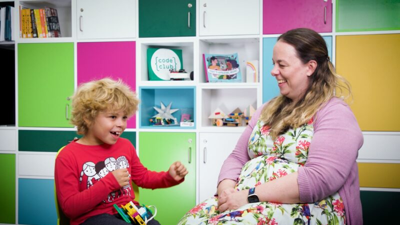
With this latest story, we’re taking you to Leeds, UK, to meet Micah, a young space enthusiast whose confidence has soared since he started attending a Code Club at his local library.
Introducing Micah
Computing skills are essential in today’s world, and Micah’s mum Catherine was keen for him to be introduced to coding from a young age.
While Micah is known to people close to him for his inquisitive nature, cheeky behaviour, and quick-witted sense of humour, he can be a little shy when meeting new people. And he isn’t always keen on his mum’s suggestions about trying new things and attending after-school clubs! However, when Catherine saw there was a Code Club running at their local library, she knew it was the perfect opportunity for Micah to try out computing.
What Catherine didn’t know is that not only would Micah find out he was a talented coder, but Code Club would also set the path for him to become a regular attendee at many of the library’s other clubs.
Opportunities for young coders
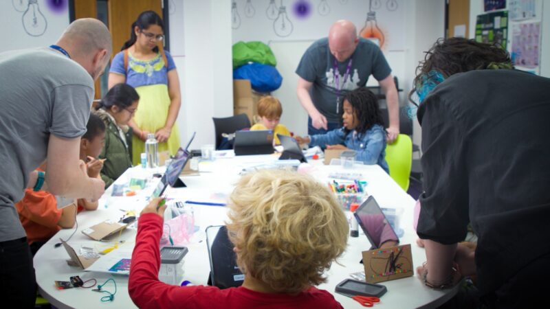
Based in Leeds, the Compton Centre Code Club is part of the Leeds Libraries network, which runs seven Code Clubs throughout the city. Liam, Senior Librarian for Digital at Leeds Libraries, described the importance of these spaces for the community and for engaging children in tech:
“Libraries are safe spaces that provide free access to exciting and innovative technology to those in our communities who might not get that opportunity. We’re proud that our Code Clubs can support young people to engage with tech, learn some new skills, and meet like-minded peers in a friendly and positive environment.
Our Code Clubs are aimed at 9- to 13-year-olds. We do have some learners that will come that have a younger sister or brother that wants to get involved as well. We never want to turn anyone away. So we’re more than welcoming for that age group to come in and have a play, get used to the equipment, and join in.”
— Liam, Senior Librarian for Digital at Leeds Libraries
Coding and confidence
Code Club provides a safe and friendly space for Micah to connect with other children, and he has embraced coding with enthusiasm. This is possible thanks to the work, support, and encouragement of Micah’s Code Club mentor Basia (they/them), the librarian at the Compton Centre who runs the club.
“Micah loves coming [to Code Club] and learning all the different things that he can do with coding. And he also loves Basia. They’re brilliant and run the club really well. It’s a super child-friendly place to be and he loves the support that he gets from them.”
– Catherine, Micah’s mum
Support from an inspiring mentor is so often an important part of a young coder’s journey, and Basia’s own journey from a coding beginner to a confident mentor highlights the positive influence Code Club has on both children and mentors.
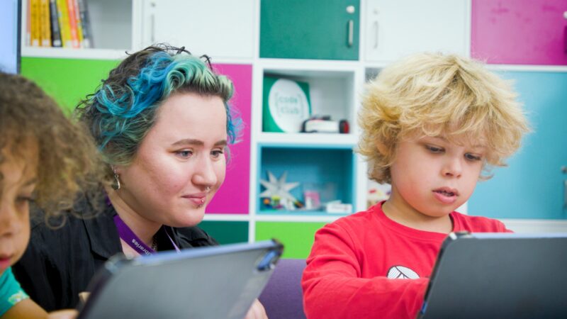
Basia reflected on how they felt when they first heard they were going to be running Code Club sessions, and how their skills and confidence have grown.
“I was daunted for a bit. But actually one of the first things I did when I started this job was to go through some of [the Raspberry Pi Foundation’s] resources and do a project in Scratch. And it was just so simple and straightforward. You know, all the resources are absolutely great and I don’t really need to think about it. I think my confidence has increased quite significantly.”
— Basia, Librarian and Code Club mentor
Since joining Code Club, Micah has become involved in other extracurricular activities, like Lego club and drama club. These experiences have contributed to Micah’s overall personal growth, showcasing the transformative power of Code Club for children.
Micah has exciting dreams for the future, including becoming an astrophysicist, a marine biologist, and the founder of a company named Save The Planet. Supported by dedicated mentors like Basia, Code Clubs are not just about teaching coding — they are helping shape the leaders of tomorrow.
Inspire young people in your community
If you are interested in encouraging your child to explore coding, take a look at the free coding project resources we have available to support you. If you would like to set up a Code Club for young people in your community, head to codeclub.org for information and support.
Help us celebrate Micah and his inspiring journey by sharing his story on X (formerly Twitter), LinkedIn, and Facebook.
The post Celebrating the community: Micah appeared first on Raspberry Pi Foundation.