Post Syndicated from Biswanath Mukherjee original https://aws.amazon.com/blogs/compute/orchestrating-big-data-processing-with-aws-step-functions-distributed-map/
Developers seek to process and enrich semi-structured big data datasets with durably orchestrated network-based workflows. For example, during quarterly earnings season, finance organizations run thousands of market simulations simultaneously to provide timely insights for scenario planning or risk management—these workloads require coordination between raw datasets and on-premise servers to provide the latest market information.
AWS Step Functions is a visual workflow service capable of orchestrating over 14,000 API actions from over 220 AWS services to build distributed applications. Now, Step Functions Distributed Map streamlines big data dataset transformation by processing Amazon Athena data manifest and Parquet files directly. Using its Distributed Map feature, you can process large scale datasets by running concurrent iterations across data entries in parallel. In Distributed mode, the Map state processes the items in the dataset in iterations called child workflow executions. You can specify the number of child workflow executions that can run in parallel. Each child workflow execution has its own, separate execution history from that of the parent workflow. By default, Step Functions runs 10,000 parallel child workflow executions in parallel.
Distributed Map can process AWS Athena data manifest and Parquet files directly, eliminating the need for custom pre-processing. You also now have visibility into your Distributed Map usage with new Amazon CloudWatch metrics: Approximate Open Map Runs Count, Open Map Run Limit, and Approximate Map Runs Backlog Size.
In this post, you’ll learn how to use AWS Step Functions Distributed Map to process Athena data manifest and Parquet files through a step-by-step demonstration.
This post is part of a series of post about AWS Step Functions Distributed Map:
|
Use case: IoT sensor data processing
You’ll build a sample application that demonstrates processing IoT sensor data in Parquet format using Step Functions Distributed Map. These Parquet data files and a manifest file containing the list of the data files are exported from Athena. The data temperature, humidity, and lbattery level from different devices. The following table shows sample of sensor data:
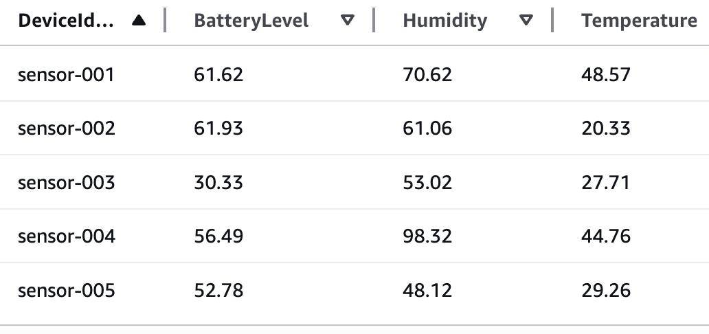
Example IoT sensor data
Your objective is to use the Athena data manifest file, get the list of Parquet files, and iterate over the data in the files to detect anomalies and also stream the processed data through Amazon Kinesis Data Firehose to an Amazon S3 bucket for further analytics using Athena queries. Following is the criteria to detect anomaly:
- Low battery conditions: less than 20%
- Humidity anomalies: more than 95% or less than 5%
- Temperature spikes: more than 35°C or less than -10°C
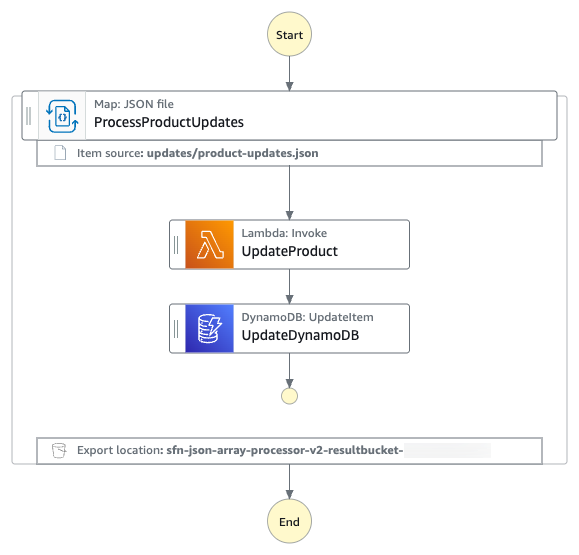
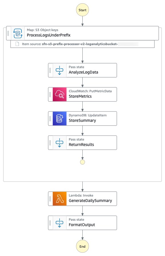
The following diagram represents the AWS Step Functions state machine:
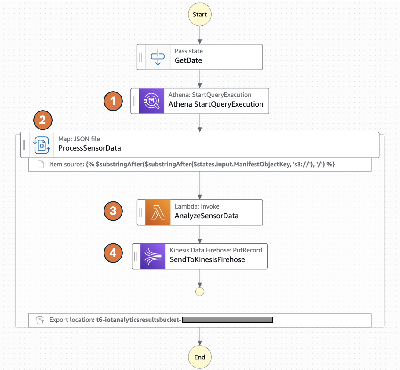
Parquet files processing workflow
- The Distributed Map runs an Athena query which generates Parquet data files and an Athena manifest file (csv). The manifest file contains the list of Parquet data files.
- Distributed Map processes these Parquet data files in parallel using child workflow executions. You can control the number of child workflow executions that can run in parallel using MaxConcurrency parameter. See Step Functions service quotas to learn more about concurrency limits.
- Each child workflow execution invokes an AWS Lambda function to process the respective Parquet file. The Lambda function processes individual sensor readings and detects anomalies according to the preceeding logic and returns a processed sensor data summary response.
- The child workflow sends the summary response record to Amazon Kinesis firehose stream which stores the results in a specified Amazon S3 results bucket.
The following Athena Start QueryExecution state runs an UNLOAD query to generate data files in Parquet format and a manifest file in CSV. The output will be stored in the S3 bucket specified in the UNLOAD query and the manifest file will be stored in the S3 bucket configured for the Athena workgroup.
The following ItemReader is configured to use a manifest type of “ATHENA_DATA” with “PARQUET” data input.
Additional supported InputType options are CSV and JSONL. All objects referenced in a single manifest file must have the same InputType format. You specify the Amazon S3 bucket location of Athena manifest CSV file under Arguments.
The context object contains information in a JSON structure about your state machine and execution. Your workflows can reference the context object in a JSONata expression with $states.context.
Within a Map state, the Context object includes the following data:
For each Map state iteration, Index contains the index number for the array item that is being currently processed, Key is available only when iterating over JSON objects, Value contains the array item being processed, and Source contains one of the following:
- For state input, the value will be : STATE_DATA
- For Amazon S3 LIST_OBJECTS_V2 with Transformation=NONE, the value will show the S3 URI for the bucket. For example: S3://amzn-s3-demo-bucket.
- For all the other input types, the value will be the Amazon S3 URI. For example: S3://amzn-s3-demo-bucket/object-key.
Using this newly introduced Source field in the context object, you can connect the child executions with the source object.
Prerequisites
- Access to an AWS account through the AWS Management Console and the AWS Command Line Interface (AWS CLI). The AWS Identity and Access Management (IAM) user that you use must have permissions to make the necessary AWS service calls and manage AWS resources mentioned in this post. While providing permissions to the IAM user, follow the principle of least-privilege.
- AWS CLI installed and configured. If you are using long-term credentials like access keys, follow manage access keys for IAM users and secure access keys for best practices.
- Git Installed
- AWS Serverless Application Model (AWS SAM) installed
- Python 3.13+ installed
Set up the state machine and sample data
Run the following steps to deploy the Step Functions state machine.
- Clone the GitHub repository in a new folder and navigate to the project root folder.
- Run the following command to install required Python dependencies for the Lambda function.
- Build the application.
- Deploy the application
- Enter the following details:
- Stack name: The CloudFormation stack name (for example, sfn-parquet-file-processor)
- AWS Region: A supported AWS Region (for example, us-east-1)
- Keep rest of the components to default values.
Note the outputs from the AWS SAM deploy. You will use them in the subsequent steps.
- Run the following command to generate sample data in csv format and upload it to an S3 bucket. Replace
<IoTDataBucketName>with the value fromsam deployouptut.
Create the Athena database and tables
Before you can run queries, you must set up an Athena database and table for your data.
- From Amazon Athena console, navigate to workgoups, select the workgroup named “primary”. Select Edit from Actions. In the query result configuration section, select the options as follows:
- Management of query results – select customer managed
- Location of query results – enter s3://<IoTDataBucketName>. Replace
<IoTDataBucketName>with the value fromsam deployoutput. - Choose Save to save the changes to the workgroup
- Select Query editor tab and run the following commands to create database and tables
- Create an Athena table in database iotsensordata that references the S3 bucket containing the raw sensor data. In this case it will be
<IoTDataBucketName>. Replace<IoTDataBucketName>with the value fromsam deployoutput. - Create an Athena table in database iotsensordata that references the S3 bucket having the analytics results streamed from Kinesis Data Firehose. Replace
<IoTAnalyticsResultsBucket>with value fromsam deployoutput. And replace<year>with the current year (e.g 2025).
Start your state machine
Now that you have data ready and Athena set up for queries, start your state machine to retrieve and process the data.
- Run the following command to start execution of the Step Functions. Replace the
<StateMachineArn>and<IoTDataBucketName>with the value from sam deploy output..The Step Functions state machine has the Athena
StartQueryExecutionstate which has anUNLOADquery that generates the sensor data files in a parquet format and a manifest file in CSV format. The manifest will have 5 rows referencing the 5 parquet files. The state machine will process these 5 parquet files in one map run. - Run the following command to get the details of the execution. Replace the
executionArnfrom the previous command. - After you see the status
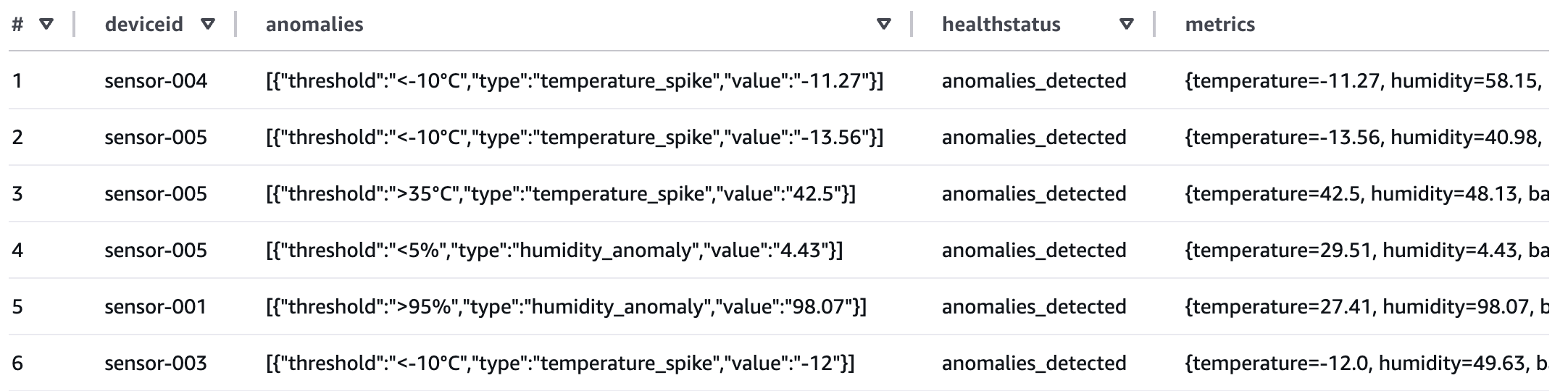
SUCCEEDED, run the following command from Athena query editor to check the processed output from Kinesis Data Firehose that was streamed to S3 bucket referenced by the Athena table created in step 4 of the preceding section.
If any of the sensor data exceeds the thresholds, the healthstatus attribute will be set to “anomalies_detected”. The workflow produced a summary table of metadata which you can now query for reporting.
Review workflow performance
Using the following observability metrics, you can review key performance behavior of your data processing workflow.
The AWS/States namespace includes the following new metrics for all Step Functions Map Runs.
OpenMapRunLimit: This is the maximum number of open Map Runs allowed in the AWS account. The default value is 1,000 runs and is a hard limit. For more information, see Quotas related to accounts.ApproximateOpenMapRunCount: This metric tracks the approximate number of Map Runs currently in progress within an account. Configuring an alarm on this metric using the Maximum statistic with a threshold of 900 or higher can help you take proactive action before reaching theOpenMapRunLimitof 1,000. This metric enables operational teams to implement preventive measures, such as staggering new executions or optimizing workflow concurrency, to maintain system stability and prevent backlog accumulation.ApproximateMapRunBacklogSize: This metric shows up when theApproximateOpenMapRunCounthas reached 1,000 and there are backlogged Map Runs waiting to be executed. Backlogged Map Runs wait at the MapRunStarted event until the total number of open Map Runs is less than the quota.
The following graph shows an example of these new metrics. Use the maximum statistic to visualize these metrics. ApproximateMapRunBacklogSize metrics appear after accounts start getting throttled on the OpenMapRunLimit limit. The OpenMapRun (orange line) is the account hard limit of 1,000 shown as a static line. The ApproximateOpenMapRunCount (violet line) is the current number of active OpenMap runs. The ApproximateMapRunBacklogSize (green line) indicates the map runs waiting in backlog to be processed. When the ApproximateOpenMapRunCount is lower than 1000 (OpenMapRun limit) there are no map runs in backlog. However, when the count reaches the OpenMapRun limit, the backlog of map runs starts to build up. After the active runs complete, the backlog will start to drain out and new runs will begin execution.
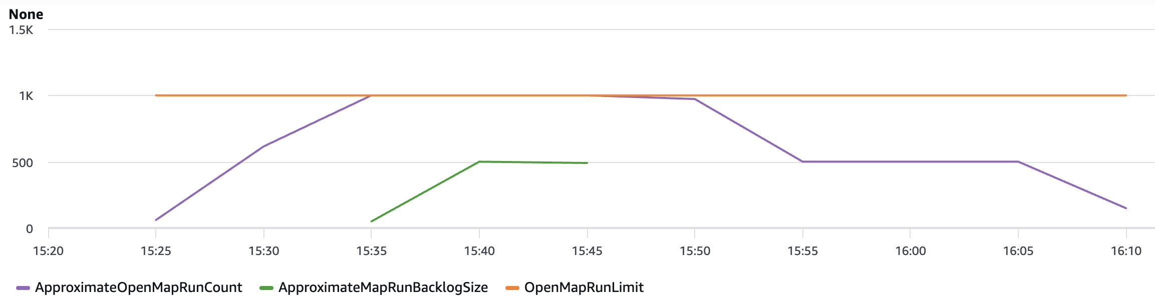
Graphed metrics from Amazon CloudWatch
Clean up
To avoid costs, remove all resources created for this post once you’re done. From the Athena query editor, run the following commands:
Run the following commands from the AWS CLI after replacing the <placeholder> variable to delete the resources you deployed for this post’s solution:
Conclusion
With this update, Distributed Map now supports additional data inputs, so you can orchestrate large-scale analytics and ETL workflows. You can now process Amazon Athena data manifest and Parquet files directly, eliminating the need for custom pre-processing. You also now have visibility into your Distributed Map usage with the following metrics: Approximate Open Map Runs Count, Open Map Run Limit, and Approximate Map Runs Backlog Size.
New input sources for Distributed Map are available in all commercial AWS Regions where AWS Step Functions is available. For a complete list of AWS Regions where Step Functions is available, see the AWS Region Table. The improved observability of your Distributed Map usage with new metrics is available in all AWS Regions. To get started, you can use the Distributed Map mode today in the AWS Step Functions console. To learn more, visit the Step Functions developer guide.
For more serverless learning resources, visit Serverless Land.