All posts by Dr. Yannick Misteli

Build a modern data architecture on AWS with Amazon AppFlow, AWS Lake Formation, and Amazon Redshift: Part 2

Post Syndicated from Dr. Yannick Misteli original https://aws.amazon.com/blogs/big-data/part-2-build-a-modern-data-architecture-on-aws-with-amazon-appflow-aws-lake-formation-and-amazon-redshift/

In Part 1 of this post, we provided a solution to build the sourcing, orchestration, and transformation of data from multiple source systems, including Salesforce, SAP, and Oracle, into a managed modern data platform. Roche partnered with AWS Professional Services to build out this fully automated and scalable platform to provide the foundation for their machine learning goals. This post continues the data journey to include the steps undertaken to build an agile and extendable Amazon Redshift data warehouse platform using a DevOps approach.

The modern data platform ingests delta changes from all source data feeds once per night. The orchestration and transformations of the data is undertaken by dbt. dbt enables data analysts and engineers to write data transformation queries in a modular manner without having to maintain the run order manually. It compiles all code into raw SQL queries that run against the Amazon Redshift cluster. It also controls the dependency management within your queries and runs it in the correct order. dbt code is a combination of SQL and Jinja (a templating language); therefore, you can express logic such as if statements, loops, filters, and macros in your queries. dbt also contains automatic data validation job scheduling to measure the data quality of the data loaded. For more information about how to configure a dbt project within an AWS environment, see Automating deployment of Amazon Redshift ETL jobs with AWS CodeBuild, AWS Batch, and DBT.

Amazon Redshift was chosen as the data warehouse because of its ability to seamlessly access data stored in industry standard open formats within Amazon Simple Storage Service (Amazon S3) and rapidly ingest the required datasets into local, fast storage using well-understood SQL commands. Being able to develop extract, load, and transform (ELT) code pipelines in SQL was important for Roche to take advantage of the existing deep SQL skills of their data engineering teams.

A modern ELT platform requires a modern, agile, and highly performant data model. The solution in this post builds a data model using the Data Vault 2.0 standards. Data Vault has several compelling advantages for data-driven organizations:

  • It removes data silos by storing all your data in reusable source system independent data stores keyed on your business keys.
  • It’s a key driver for data integration at many levels, from multiple source systems, multiple local markets, multiple companies and affiliates, and more.
  • It reduces data duplication. Because data is centered around business keys, if more than one system sends the same data, then multiple data copies aren’t needed.
  • It holds all history from all sources; downstream you can access any data at any point in time.
  • You can load data without contention or in parallel, and in batch or real time.
  • The model can adapt to change with minimal impact. New business relationships can be made independently of the existing relationships
  • The model is well established in the industry and naturally drives templated and reusable code builds.

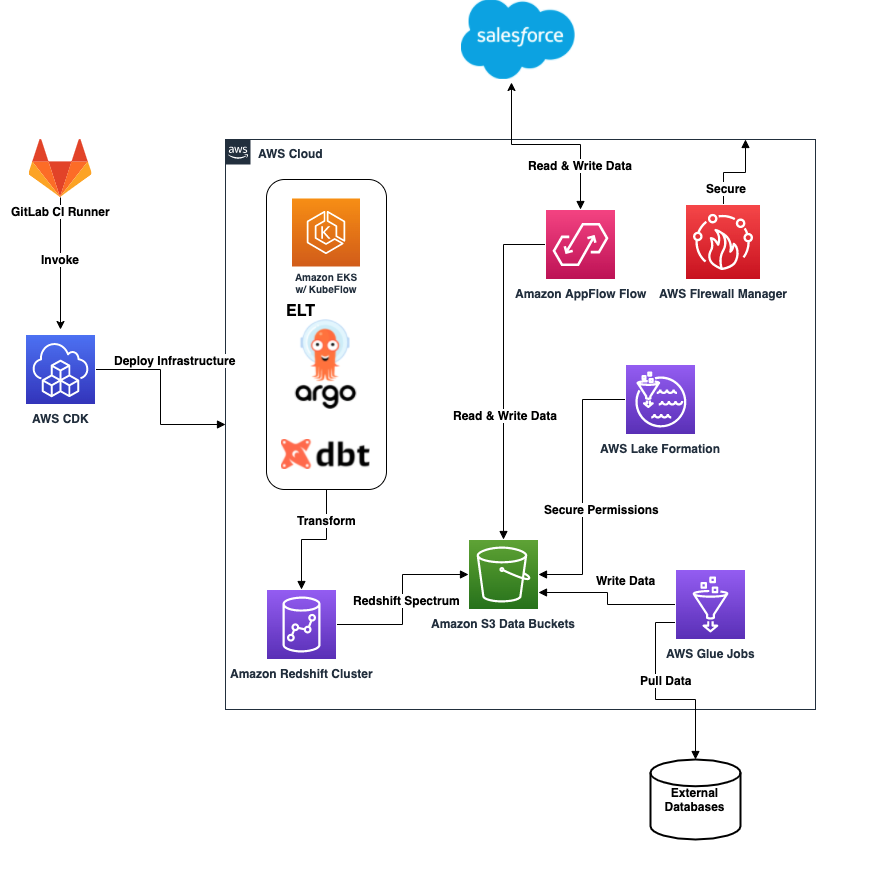
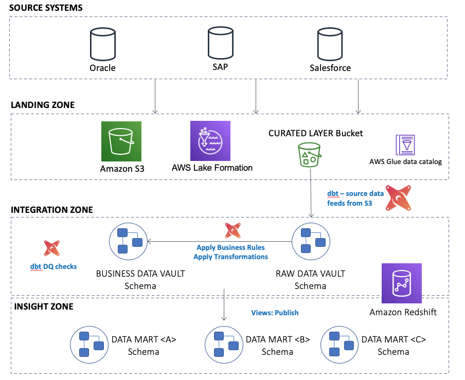
The following diagram illustrates the high-level overview of the architecture:

Amazon Redshift has several methods for ingesting data from Amazon S3 into the data warehouse cluster. For this modern data platform, we use a combination of the following methods:

  • We use Amazon Redshift Spectrum to read data directly from Amazon S3. This allows the project to rapidly load, store, and use external datasets. Amazon Redshift allows the creation of external schemas and external tables to facilitate data being accessed using standard SQL statements.
  • Some feeds are persisted in a staging schema within Amazon Redshift, for example larger data volumes and datasets that are used multiple times in subsequent ELT processing. dbt handles the orchestration and loading of this data in an incremental manner to cater to daily delta changes.

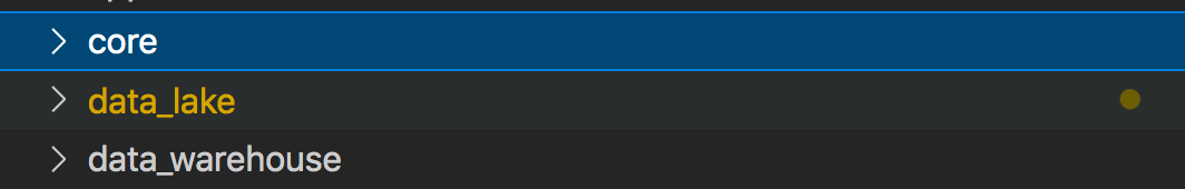
Within Amazon Redshift, the Data Vault 2.0 data model is split into three separate areas:

  • Raw Data Vault within a schema called raw_dv
  • Business Data Vault within a schema called business_dv
  • Multiple Data Marts, each with their own schema

Raw Data Vault

Business keys are central to the success of any Data Vault project, and we created hubs within Amazon Redshift as follows:

CREATE TABLE IF NOT EXISTS raw_dv.h_user
(
 user_pk          VARCHAR(32)   			 
,user_bk          VARCHAR(50)   			 
,load_dts         TIMESTAMP  	 
,load_source_dts  TIMESTAMP  	 
,bookmark_dts     TIMESTAMP  	 
,source_system_cd VARCHAR(10)   				 
) 
DISTSTYLE ALL;

Keep in mind the following:

  • The business keys from one or more source feeds are written to the reusable _bk column; compound business keys should be concatenated together with a common separator between each element.
  • The primary key is stored in the _pk column and is a hashed value of the _bk column. In this case, MD5 is the hashing algorithm used.
  • Load_Dts is the date and time of the insertion of this row.
  • Hubs hold reference data, which is typically smaller in volume than transactional data, so you should choose a distribution style of ALL for the most performant joining to other tables at runtime.

Because Data Vault is built on a common reusable notation, the dbt code is parameterized for each target. The Roche engineers built a Yaml-driven code framework to parameterize the logic for the build of each target table, enabling rapid build and testing of new feeds. For example, the preceding user hub contains parameters to identify source columns for the business key, source to target mappings, and physicalization choices for the Amazon Redshift target:

name: h_user
    type: hub
    materialized: incremental
    schema: raw_dv
    dist: all
    pk_name: user_pk
    bk:
      name: user_bk
      type: varchar(50)
    sources:
      - name: co_rems_invitee
        schema: re_rems_core
        key:
          - dwh_source_country_cd
          - employee_user_id
        columns:
          - source: "'REMS'"
            alias: source_system_cd
            type: varchar(10)
        load_source_dts: glue_dts
        bookmark_dts: bookmark_dts        
      - name: co_rems_event_users
        schema: re_rems_core
        key:
          - dwh_source_country_cd
          - user_name
        columns:
          - source: "'REMS'"
            alias: source_system_cd
            type: varchar(10)
        load_source_dts: glue_dts
        bookmark_dts: bookmark_dts        
      - name: user
        alias: user_by_id
        schema: roche_salesforce_we_prod
        key:
          - id
        columns:
          - source: "'SFDC_WE'"
            alias: source_system_cd
            type: varchar(10)
        load_source_dts: to_date(appflow_date_str,'YYYYMMDD')
        bookmark_dts: to_date(systemmodstamp,'YYYY-MM-DD HH24.mi.ss')
        where: id > 0 and id <> '' and usertype = 'Standard'
      - name: activity_g__c
        schema: roche_salesforce_we_prod
        key:
          - ownerid
        columns:
          - source: "'SFDC_WE'"
            alias: source_system_cd
            type: varchar(10)
        load_source_dts: to_date(appflow_date_str,'YYYYMMDD')
        bookmark_dts: to_date(systemmodstamp,'YYYY-MM-DD HH24.mi.ss')        
      - name: user_territory_g__c
        schema: roche_salesforce_we_prod
        key:
          - user_ref_g__c
        columns:
          - source: "'SFDC_WE'"
            alias: source_system_cd
            type: varchar(10)
        load_source_dts: to_date(appflow_date_str,'YYYYMMDD')
        bookmark_dts: to_date(systemmodstamp,'YYYY-MM-DD HH24.mi.ss')

On reading the YAML configuration, dbt outputs the following, which is run against the Amazon Redshift cluster:

{# Script generated by dbt model generator #}

{{
	config({
	  "materialized": "incremental",
	  "schema": "raw_dv",
	  "dist": "all",
	  "unique_key": "user_pk",
	  "insert_only": {}
	})
}}

with co_rems_invitee as (

	select
		{{ hash(['dwh_source_country_cd', 'employee_user_id'], 'user_pk') }},
		cast({{ compound_key(['dwh_source_country_cd', 'employee_user_id']) }} as varchar(50)) as user_bk,
		{{ dbt_utils.current_timestamp() }} as load_dts,
		glue_dts as load_source_dts,
		bookmark_dts as bookmark_dts,
		cast('REMS' as varchar(10)) as source_system_cd
	from
		{{ source('re_rems_core', 'co_rems_invitee') }}
	where
		dwh_source_country_cd is not null 
		and employee_user_id is not null

		{% if is_incremental() %}
			and glue_dts > (select coalesce(max(load_source_dts), to_date('20000101', 'yyyymmdd', true)) from {{ this }})
		{% endif %}

), 
co_rems_event_users as (

	select
		{{ hash(['dwh_source_country_cd', 'user_name'], 'user_pk') }},
		cast({{ compound_key(['dwh_source_country_cd', 'user_name']) }} as varchar(50)) as user_bk,
		{{ dbt_utils.current_timestamp() }} as load_dts,
		glue_dts as load_source_dts,
		bookmark_dts as bookmark_dts,
		cast('REMS' as varchar(10)) as source_system_cd
	from
		{{ source('re_rems_core', 'co_rems_event_users') }}
	where
		dwh_source_country_cd is not null 
		and user_name is not null

		{% if is_incremental() %}
			and glue_dts > (select coalesce(max(load_source_dts), to_date('20000101', 'yyyymmdd', true)) from {{ this }})
		{% endif %}

), 
all_sources as (

	select * from co_rems_invitee
	union
	select * from co_rems_event_users

),
unique_key as (

	select
		row_number() over(partition by user_pk order by bookmark_dts desc) as rn,
		user_pk,
		user_bk,
		load_dts,
		load_source_dts,
		bookmark_dts,
		source_system_cd
	from
		all_sources

)
select
	user_pk,
	user_bk,
	load_dts,
	load_source_dts,
	bookmark_dts,
	source_system_cd
from
	unique_key
where
	rn = 1

dbt also has the capability to add reusable macros to allow common tasks to be automated. The following example shows the construction of the business key with appropriate separators (the macro is called compound_key):

{% macro single_key(field) %}
  {# Takes an input field value and returns a trimmed version of it. #}
  NVL(NULLIF(TRIM(CAST({{ field }} AS VARCHAR)), ''), '@@')
{% endmacro %}

{% macro compound_key(field_list,sort=none) %}
  {# Takes an input field list and concatenates it into a single column value.
     NOTE: Depending on the sort parameter [True/False] the input field
     list has to be passed in a correct order if the sort parameter
     is set to False (default option) or the list will be sorted 
     if You will set up the sort parameter value to True #}
  {% if sort %}
    {% set final_field_list = field_list|sort %}
  {%- else -%}
    {%- set final_field_list = field_list -%}
  {%- endif -%}        
  {% for f in final_field_list %}
    {{ single_key(f) }}
    {% if not loop.last %} || '^^' || {% endif %}
  {% endfor %}
{% endmacro %}

{% macro hash(columns=none, alias=none, algorithm=none) %}
    {# Applies a Redshift supported hash function to the input string 
       or list of strings. #}

    {# If single column to hash #}
    {% if columns is string %}
        {% set column_str = single_key(columns) %}
        {{ redshift__hash(column_str, alias, algorithm) }}
    {# Else a list of columns to hash #}
    {% elif columns is iterable %}        
        {% set column_str = compound_key(columns) %}
        {{ redshift__hash(column_str, alias, algorithm) }}
    {% endif %}
   
{% endmacro %}

{% macro redshift__hash(column_str, alias, algorithm) %}
    {# Applies a Redshift supported hash function to the input string. #}

    {# If the algorithm is none the default project configuration for hash function will be used. #}
    {% if algorithm == none or algorithm not in ['MD5', 'SHA', 'SHA1', 'SHA2', 'FNV_HASH'] %}
        {# Using MD5 if the project variable is not defined. #}
        {% set algorithm = var('project_hash_algorithm', 'MD5') %}
    {% endif %}

    {# Select hashing algorithm #}
    {% if algorithm == 'FNV_HASH' %}
        CAST(FNV_HASH({{ column_str }}) AS BIGINT) AS {{ alias }}
    {% elif algorithm == 'MD5' %}
        CAST(MD5({{ column_str }}) AS VARCHAR(32)) AS {{ alias }}
    {% elif algorithm == 'SHA' or algorithm == 'SHA1' %}
        CAST(SHA({{ column_str }}) AS VARCHAR(40)) AS {{ alias }}
    {% elif algorithm == 'SHA2' %}
        CAST(SHA2({{ column_str }}, 256) AS VARCHAR(256)) AS {{ alias }}
    {% endif %}

{% endmacro %}

Historized reference data about each business key is stored in satellites. The primary key of each satellite is a compound key consisting of the _pk column of the parent hub and the Load_Dts. See the following code:

CREATE TABLE IF NOT EXISTS raw_dv.s_user_reine2
(
 user_pk             VARCHAR(32)   			 
,load_dts            TIMESTAMP    	 
,hash_diff           VARCHAR(32)   			 
,load_source_dts     TIMESTAMP  	 
,bookmark_dts        TIMESTAMP    	 
,source_system_cd    VARCHAR(10)				 
,is_deleted          VARCHAR(1)   				 
,invitee_type        VARCHAR(10)   			 
,first_name          VARCHAR(50)   			 
,last_name           VARCHAR(10)   			 
)
DISTSTYLE ALL
SORTKEY AUTO;

CREATE TABLE IF NOT EXISTS raw_dv.s_user_couser
(
 user_pk                VARCHAR(32)   			 
,load_dts               TIMESTAMP  	 
,hash_diff              VARCHAR(32)   			 
,load_source_dts        TIMESTAMP  	 
,bookmark_dts           TIMESTAMP  	 
,source_system_cd       VARCHAR(10)   			 
,name                   VARCHAR(150)   			 
,username               VARCHAR(80)   			 
,firstname              VARCHAR(40)   			 
,lastname               VARCHAR(80)   			 
,alias                  VARCHAR(8)   				 
,community_nickname     VARCHAR(30)   			 
,federation_identifier  VARCHAR(50)   			 
,is_active              VARCHAR(10)   			 
,email                  VARCHAR(130)   			 
,profile_name           VARCHAR(80)   			 
)
DISTSTYLE ALL
SORTKEY AUTO;

Keep in mind the following:

  • The feed name is saved as part of the satellite name. This allows the loading of reference data from either multiple feeds within the same source system or from multiple source systems.
  • Satellites are insert only; new reference data is loaded as a new row with an appropriate Load_Dts.
  • The HASH_DIFF column is a hashed concatenation of all the descriptive columns within the satellite. The dbt code uses it to decide whether reference data has changed and a new row is to be inserted.
  • Unless the data volumes within a satellite become very large (millions of rows), you should choose a distribution choice of ALL to enable the most performant joins at runtime. For larger volumes of data, choose a distribution style of AUTO to take advantage of Amazon Redshift automatic table optimization, which chooses the most optimum distribution style and sort key based on the downstream usage of these tables.

Transactional data is stored in a combination of link and link satellite tables. These tables hold the business keys that contribute to the transaction being undertaken as well as optional measures describing the transaction.

Previously, we showed the build of the user hub and two of its satellites. In the following link table, the user hub foreign key is one of several hub keys in the compound key:

CREATE TABLE IF NOT EXISTS raw_dv.l_activity_visit
(
 activity_visit_pk         VARCHAR(32)   			 
,activity_pk               VARCHAR(32)   			 
,activity_type_pk          VARCHAR(32)   			
,hco_pk                    VARCHAR(32)   			
,address_pk                VARCHAR(32)   			
,user_pk                   VARCHAR(32)   			
,hcp_pk                    VARCHAR(32)   			
,brand_pk                  VARCHAR(32)   			
,activity_attendee_pk      VARCHAR(32)   			
,activity_discussion_pk    VARCHAR(32)				
,load_dts                  TIMESTAMP  	
,load_source_dts           TIMESTAMP  				
,bookmark_dts              TIMESTAMP  				
,source_system_cd          VARCHAR(10)   				
)
DISTSTYLE KEY
DISTKEY (activity_visit_pk)
SORTKEY (activity_visit_pk);

Keep in mind the following:

  • The foreign keys back to each hub are a hash value of the business keys, giving a 1:1 join with the _pk column of each hub.
  • The primary key of this link table is a hash value of all of the hub foreign keys.
  • The primary key gives direct access to the optional link satellite that holds further historized data about this transaction. The definition of the link satellites is almost identical to satellites; instead of the _pk from the hub being part of the compound key, the _pk of the link is used.
  • Because data volumes are typically larger for links and link satellites than hubs or satellites, you can again choose AUTO distribution style to let Amazon Redshift choose the optimum physical table distribution choice. If you do choose a distribution style, then choose KEY on the _pk column for both the distribution style and sort key on both the link and any link satellites. This improves downstream query performance by co-locating the datasets on the same slice within the compute nodes and enables MERGE JOINS at run time for optimum performance.

In addition to the dbt code to build all the preceding targets in the Amazon Redshift schemas, the product contains a powerful testing tool that makes assertions on the underlying data contents. The platform continuously tests the results of each data load.

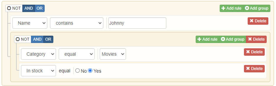
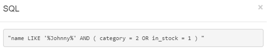
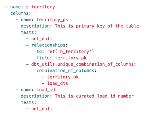
Tests are specified using a YAML file called schema.yml. For example, taking the territory satellite (s_territory), we can see automated testing for conditions, including ensuring the primary key is populated, its parent key is present in the territory hub (h_territory), and the compound key of this satellite is unique:

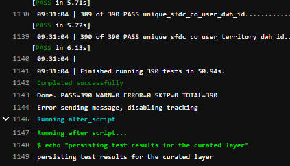
As shown in the following screenshot, the tests are clearly labeled as PASS or FAILED for quick identification of data quality issues.

Business Data Vault

The Business Data Vault is a vital element of any Data Vault model. This is the place where business rules, KPI calculations, performance denormalizations, and roll-up aggregations take place. Business rules can change over time, but the raw data does not, which is why the contents of the Raw Data Vault should never be modified.

The type of objects created in the Business Data Vault schema include the following:

  • Type 2 denormalization based on either the latest load date timestamp or a business-supplied effective date timestamp. These objects are ideal as the base for a type 2 dimension view within a data mart.
  • Latest row filtering based on either the latest load date timestamp or a business-supplied effective date timestamp. These objects are ideal as the base for a type 1 dimension within a data mart.
  • For hubs with multiple independently loaded satellites, point-in-time (PIT) tables are created with the snapshot date set to one time per day.
  • Where the data access requirements span multiple links and link satellites, bridge tables are created with the snapshot date set to one time per day.

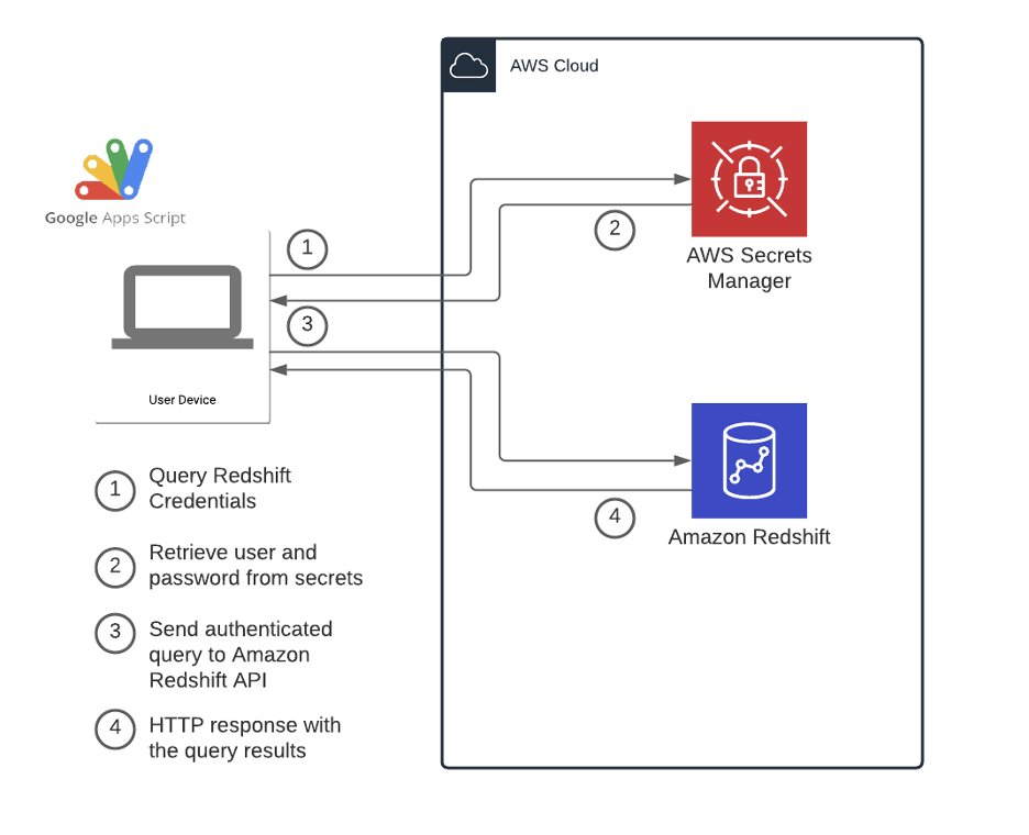
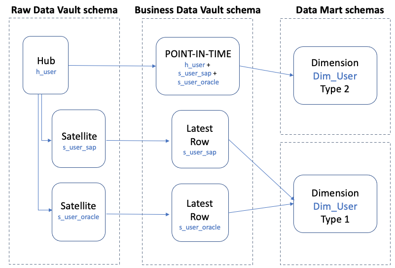
In the following diagram, we show an example of user reference data from two source systems being loaded into separate satellite targets.

In this example, we show User reference data from two source systems being loaded into separate Satellite targets

Keep in mind the following:

  • You should create a separate schema for the Business Data Vault objects
  • You can build several object types in the Business Data Vault:
    • PIT and bridge targets are typically either tables or materialized views can be used for data that incrementally changes due to the auto refresh capabilities
    • The type 2 and latest row selections from an underlying satellite are typically views because of the lower data volumes typically found in reference datasets
  • Because the Raw Data Vault tables are insert only, to determine a timeline of changes, create a view similar to the following:
CREATE OR REPLACE VIEW business_dv.ref_user_type2 AS
SELECT 
  s.user_pk,
  s.load_dts from_dts,
  DATEADD(second,-1,COALESCE(LEAD(s.load_dts) OVER (PARTITION BY s.user_pk ORDER BY s.load_dts),'2200-01-01 00:00:00')) AS to_dts
  FROM raw_dv.s_user_reine2 s
  INNER JOIN raw_dv.h_user h ON h.user_pk = s.user_pk
  WITH NO SCHEMA BINDING;

Data Marts

The work undertaken in the Business Data Vault means that views can be developed within the Data Marts to directly access the data without having to physicalize the results into another schema. These views may apply filters to the Business Vault objects, for example to filter only for data from specific countries, or the views may choose a KPI that has been calculated in the Business Vault that is only useful within this one data mart.

Conclusion

In this post, we detailed how you can use dbt and Amazon Redshift for continuous build and validation of a Data Vault model that stores all data from multiple sources in a source-independent manner while offering flexibility and choice of subsequent business transformations and calculations.

Special thanks go to Roche colleagues Bartlomiej Zalewski, Wojciech Kostka, Michalina Mastalerz, Kamil Piotrowski, Igor Tkaczyk, Andrzej Dziabowski, Joao Antunes, Krzysztof Slowinski, Krzysztof Romanowski, Patryk Szczesnowicz, Jakub Lanski, and Chun Wei Chan for their project delivery and support with this post.


About the Authors

Dr. Yannick Misteli, Roche – Dr. Yannick Misteli is leading cloud platform and ML engineering teams in global product strategy (GPS) at Roche. He is passionate about infrastructure and operationalizing data-driven solutions, and he has broad experience in driving business value creation through data analytics.

Simon Dimaline, AWS – Simon Dimaline has specialised in data warehousing and data modelling for more than 20 years. He currently works for the Data & Analytics team within AWS Professional Services, accelerating customers’ adoption of AWS analytics services.

Matt Noyce, AWS – Matt Noyce is a Senior Cloud Application Architect in Professional Services at Amazon Web Services. He works with customers to architect, design, automate, and build solutions on AWS for their business needs.

Chema Artal Banon, AWS – Chema Artal Banon is a Security Consultant at AWS Professional Services and he works with AWS’s customers to design, build, and optimize their security to drive business. He specializes in helping companies accelerate their journey to the AWS Cloud in the most secure manner possible by helping customers build the confidence and technical capability.

Build a modern data architecture on AWS with Amazon AppFlow, AWS Lake Formation, and Amazon Redshift.

Post Syndicated from Dr. Yannick Misteli original https://aws.amazon.com/blogs/big-data/build-a-modern-data-architecture-on-aws-with-amazon-appflow-aws-lake-formation-and-amazon-redshift/

This is a guest post written by Dr. Yannick Misteli, lead cloud platform and ML engineering in global product strategy (GPS) at Roche.

Recently the Roche Data Insights (RDI) initiative was launched to achieve our vision using new ways of working and collaboration in order to build shared, interoperable data & insights with federated governance. Furthermore, a simplified & integrated data landscape shall be established in order to empower insights communities. One of the first domains to engage in this program is the Go-to-Market (GTM) area which comprises sales, marketing, medical access and market affairs in Roche. GTM domain enables Roche to understand customers and to ultimately create and deliver valuable services that meet their needs. GTM as a domain extends beyond health care professionals (HCPs) to a larger healthcare ecosystem consisting of patients, communities, health authorities, payers, providers, academia, competitors, so on and so forth. Therefore, Data & Analytics are key in supporting the internal and external stakeholders in their decision-making processes through actionable insights.

Roche GTM built a modern data and machine learning (ML) platform on AWS while utilizing DevOps best practices. The mantra of everything as code (EaC) was key in building a fully automated, scalable data lake and data warehouse on AWS.

In this this post, you learn about how Roche used AWS products and services such as Amazon AppFlow, AWS Lake Formation, and Amazon Redshift to provision and populate their data lake; how they sourced, transformed, and loaded data into the data warehouse; and how they realized best practices in security and access control.

In the following sections, you dive deep into the scalable, secure, and automated modern data platform that Roche has built. We demonstrate how to automate data ingestion, security standards, and utilize DevOps best practices to ease management of your modern data platform on AWS.

Data platform architecture

The following diagram illustrates the data platform architecture.

The architecture contains the following components:

Lake Formation security

We use Lake Formation to secure all data as it lands in the data lake. Separating each data lake layer into distinct S3 buckets and prefixes enables fine-grained access control policies that Lake Formation implements. This concept also extends to locking down access to specific rows and columns and applying policies to specific IAM roles and users. Governance and access to data lake resources is difficult to manage, but Lake Formation simplifies this process for administrators.

To secure access to the data lake using Lake Formation, the following steps are automated using the AWS CDK with customized constructs:

  1. Register the S3 data buckets and prefixes, and corresponding AWS Glue databases with Lake Formation.
  2. Add data lake administrators (GitLab runner IAM deployment role and administrator IAM role).
  3. Grant the AWS Glue job IAM roles access to the specific AWS Glue databases.
  4. Grant the AWS Lambda IAM role access to the Amazon AppFlow databases.
  5. Grant the listed IAM roles access to the corresponding tables in the AWS Glue databases.

AWS Glue Data Catalog

The AWS Glue Data Catalog is the centralized registration and access point for all databases and tables that are created in both the data lake and in Amazon Redshift. This provides centralized transparency to all resources along with their schemas and the location of all data that is referenced. This is a critical aspect for any data operations performed within the lake house platform.

Data sourcing and ingestion

Data is sourced and loaded into the data lake through the use of AWS Glue jobs and Amazon AppFlow. The ingested data is made available in the Amazon Redshift data warehouse through Amazon Redshift Spectrum using external schemas and tables. The process of creating the external schemas and linking it to the Data Catalog is outlined later in this post.

Amazon AppFlow Salesforce ingestion

Amazon AppFlow is a fully-managed integration service that allows you to pull data from sources such as Salesforce, SAP, and Zendesk. Roche integrates with Salesforce to load Salesforce objects securely into their data lake without needing to write any custom code. Roche also pushes ML results back to Salesforce using Amazon AppFlow to facilitate the process.

Salesforce objects are first fully loaded into Amazon S3 and then are flipped to a daily incremental load to capture deltas. The data lands in the raw zone bucket in Parquet format using the date as a partition. The Amazon AppFlow flows are created through the use of a YAML configuration file (see the following code). This configuration is consumed by the AWS CDK deployment to create the corresponding flows.

appflow:
  flow_classes:
    salesforce:
      source: salesforce
      destination: s3
      incremental_load: 1
      schedule_expression: "rate(1 day)"
      s3_prefix: na
      connector_profile: roche-salesforce-connector-profile1,roche-salesforce-connector-profile2
      description: appflow flow flow from Salesforce
      environment: all
  - name: Account
    incremental_load: 1
    bookmark_col: appflow_date_str
  - name: CustomSalesforceObject
    pii: 0
    bookmark_col: appflow_date_str
    upsert_field_list: upsertField
    s3_prefix: prefix
    source: s3
    destination: salesforce
    schedule_expression: na
    connector_profile: roche-salesforce-connector-profile

The YAML configuration makes it easy to select whether data should be loaded from an S3 bucket back to Salesforce or from Salesforce to an S3 bucket. This configuration is subsequently read by the AWS CDK app and corresponding stacks to translate into Amazon AppFlow flows.

The following options are specified in the preceding YAML configuration file:

  • source – The location to pull data from (Amazon S3, Salesforce)
  • destination – The destination to put data to (Amazon S3, Salesforce)
  • object_name – The name of the Salesforce object to interact with
  • incremental_load – A Boolean specifying if the load should be incremental or full (0 means full, 1 means incremental)
  • schedule_expression – The cron or rate expression to run the flow (na makes it on demand)
  • s3_prefix – The prefix to push or pull the data from in the S3 bucket
  • connector_profile – The Amazon AppFlow connector profile name to use when connecting to Salesforce (can be a CSV list)
  • environment – The environment to deploy this Amazon AppFlow flow to (all means deploy to dev and prod, dev means development environment, prod means production environment)
  • upsert_field_list – The set of Salesforce object fields (can be a CSV list) to use when performing an upsert operation back to Salesforce (only applicable when loaded data back from an S3 bucket back to Salesforce)
  • bookmark_col – The name of the column to use in the Data Catalog for registering the daily load date string partition

Register Salesforce objects to the Data Catalog

Complete the following steps to register data loaded into the data lake with the Data Catalog and link it to Amazon Redshift:

  1. Gather Salesforce object fields and corresponding data types.
  2. Create a corresponding AWS Glue database in the Data Catalog.
  3. Run a query against Amazon Redshift to create an external schema that links to the AWS Glue database.
  4. Create tables and partitions in the AWS Glue database and tables.

Data is accessible via the Data Catalog and the Amazon Redshift cluster.

Amazon AppFlow dynamic field gathering

To construct the schema of the loaded Salesforce object in the data lake, you invoke the following Python function. The code utilizes an Amazon AppFlow client from Boto3 to dynamically gather the Salesforce object fields to construct the Salesforce object’s schema.

import boto3

client = boto3.client('appflow')

def get_salesforce_object_fields(object_name: str, connector_profile: str):
    """
    Gathers the Salesforce object and its corresponding fields.

    Parameters:
        salesforce_object_name (str) = the name of the Salesforce object to consume.
        appflow_connector_profile (str) = the name of AppFlow Connector Profile.

    Returns:
        object_schema_list (list) =  a list of the object's fields and datatype (a list of dictionaries).
    """
    print("Gathering Object Fields")

    object_fields = []

    response = client.describe_connector_entity(
        connectorProfileName=connector_profile,
        connectorEntityName=object_name,
        connectorType='Salesforce'
    )

    for obj in response['connectorEntityFields']:
        object_fields.append(
            {'field': obj['identifier'], 'data_type': obj['supportedFieldTypeDetails']['v1']['fieldType']})

    return object_fields

We use the function for both the creation of the Amazon AppFlow flow via the AWS CDK deployment and for creating the corresponding table in the Data Catalog in the appropriate AWS Glue database.

Create an Amazon CloudWatch Events rule, AWS Glue table, and partition

To add new tables (one per Salesforce object loaded into Amazon S3) and partitions into the Data Catalog automatically, you create an Amazon CloudWatch Events rule. This function enables you to query the data in both AWS Glue and Amazon Redshift.

After the Amazon AppFlow flow is complete, it invokes a CloudWatch Events rule and a corresponding Lambda function to either create a new table in AWS Glue or add a new partition with the corresponding date string for the current day. The CloudWatch Events rule looks like the following screenshot.

The invoked Lambda function uses the Amazon SageMaker Data Wrangler Python package to interact with the Data Catalog. Using the preceding function definition, the object fields and their data types are accessible to pass to the following function call:

import awswrangler as wr

def create_external_parquet_table(
    database_name: str, 
    table_name: str, 
    s3_path: str, 
    columns_map: dict, 
    partition_map: dict
):
    """
    Creates a new external table in Parquet format.

    Parameters:
        database_name (str) = the name of the database to create the table in.
        table_name (str) = the name of the table to create.
        s3_path (str) = the S3 path to the data set.
        columns_map (dict) = a dictionary object containing the details of the columns and their data types from appflow_utility.get_salesforce_object_fields
        partition_map (dict) = a map of the paritions for the parquet table as {'column_name': 'column_type'}
    
    Returns:
        table_metadata (dict) = metadata about the table that was created.
    """

    column_type_map = {}

    for field in columns_map:
        column_type_map[field['name']] = field['type']

    return wr.catalog.create_parquet_table(
        database=database_name,
        table=table_name,
        path=s3_path,
        columns_types=column_type_map,
        partitions_types=partition_map,
        description=f"AppFlow ingestion table for {table_name} object"
    )

If the table already exists, the Lambda function creates a new partition to account for the date in which the flow completed (if it doesn’t already exist):

import awswrangler as wr

def create_parquet_table_date_partition(
    database_name: str, 
    table_name: str, 
    s3_path: str, 
    year: str, 
    month: str, 
    day: str
):
    """
    Creates a new partition by the date (YYYY-MM-DD) on an existing parquet table.

    Parameters:
        database_name (str) = the name of the database to create the table in.
        table_name (str) = the name of the table to create.
        s3_path (str) = the S3 path to the data set.
        year(str) = the current year for the partition (YYYY format).
        month (str) = the current month for the partition (MM format).
        day (str) = the current day for the partition (DD format).
    
    Returns:
        table_metadata (dict) = metadata about the table that has a new partition
    """

    date_str = f"{year}{month}{day}"
    
    return wr.catalog.add_parquet_partitions(
        database=database_name,
        table=table_name,
        partitions_values={
            f"{s3_path}/{year}/{month}/{day}": [date_str]
        }
    )
    
def table_exists(
    database_name: str, 
    table_name: str
):
    """
    Checks if a table exists in the Glue catalog.

    Parameters:
        database_name (str) = the name of the Glue Database where the table should be.
        table_name (str) = the name of the table.
    
    Returns:
        exists (bool) = returns True if the table exists and False if it does not exist.
    """

    try:
        wr.catalog.table(database=database_name, table=table_name)
        return True
    except ClientError as e:
        return False

Amazon Redshift external schema query

An AWS Glue database is created for each Amazon AppFlow connector profile that is present in the preceding configuration. The objects that are loaded from Salesforce into Amazon S3 are registered as tables in the Data Catalog under the corresponding database. To link the database in the Data Catalog with an external Amazon Redshift schema, run the following query:

CREATE EXTERNAL SCHEMA ${connector_profile_name}_ext from data catalog
database '${appflow_connector_profile_name}'
iam_role 'arn:aws:iam::${AWS_ACCOUNT_ID}:role/RedshiftSpectrumRole'
region 'eu-west-1';

The specified iam_role value must be an IAM role created ahead of time and must have the appropriate access policies specified to query the Amazon S3 location.

Now, all the tables available in the Data Catalog can be queried using SQL locally in Amazon Redshift Spectrum.

Amazon AppFlow Salesforce destination

Roche trains and invokes ML models using data found in the Amazon Redshift data warehouse. After the ML models are complete, the results are pushed back into Salesforce. Through the use of Amazon AppFlow, we can achieve the data transfer without writing any custom code. The schema of the results must match the schema of the corresponding Salesforce object, and the format of the results must be written in either JSON lines or CSV format in order to be written back into Salesforce.

AWS Glue Jobs

To source on-premises data feeds into the data lake, Roche has built a set of AWS Glue jobs in Python. There are various external sources including databases and APIs that are directly loaded into the raw zone S3 bucket. The AWS Glue jobs are run on a daily basis to load new data. The data that is loaded follows the partitioning scheme of YYYYMMDD format in order to more efficiently store and query datasets. The loaded data is then converted into Parquet format for more efficient querying and storage purposes.

Amazon EKS and KubeFlow

To deploy ML models on Amazon EKS, Roche uses Kubeflow on Amazon EKS. The use of Amazon EKS as the backbone infrastructure makes it easy to build, train, test, and deploy ML models and interact with Amazon Redshift as a data source.

Firewall Manager

As an added layer of security, Roche takes extra precautions through the use of Firewall Manager. This allows Roche to explicitly deny or allow inbound and outbound traffic through the use of stateful and stateless rule sets. This also enables Roche to allow certain outbound access to external websites and deny websites that they don’t want resources inside of their Amazon VPC to have access to. This is critical especially when dealing with any sensitive datasets to ensure that data is secured and has no chance of being moved externally.

CI/CD

All the infrastructure outlined in the architecture diagram was automated and deployed to multiple AWS Regions using a continuous integration and continuous delivery (CI/CD) pipeline with GitLab Runners as the orchestrator. The GitFlow model was used for branching and invoking automated deployments to the Roche AWS accounts.

Infrastructure as code and AWS CDK

Infrastructure as code (IaC) best practices were used to facilitate the creation of all infrastructure. The Roche team uses the Python AWS CDK to deploy, version, and maintain any changes that occur to the infrastructure in their AWS account.

AWS CDK project structure

The top level of the project structure in GitLab includes the following folders (while not limited to just these folders) in order to keep infrastructure and code all in one location.

To facilitate the various resources that are created in the Roche account, the deployment was broken into the following AWS CDK apps, which encompass multiple stacks:

  • core
  • data_lake
  • data_warehouse

The core app contains all the stacks related to account setup and account bootstrapping, such as:

  • VPC creation
  • Initial IAM roles and policies
  • Security guardrails

The data_lake app contains all the stacks related to creating the AWS data lake, such as:

  • Lake Formation setup and registration
  • AWS Glue database creation
  • S3 bucket creation
  • Amazon AppFlow flow creation
  • AWS Glue job setup

The data_warehouse app contains all the stacks related to setting up the data warehouse infrastructure, such as:

  • Amazon Redshift cluster
  • Load balancer to Amazon Redshift cluster
  • Logging

The AWS CDK project structure described was chosen to keep the deployment flexible and to logically group together stacks that relied on each other. This flexibility allows for deployments to be broken out by function and deployed only when truly required and needed. This decoupling of different parts of the provisioning maintains flexibility when deploying.

AWS CDK project configuration

Project configurations are flexible and extrapolated away as YAML configuration files. For example, Roche has simplified the process of creating a new Amazon AppFlow flow and can add or remove flows as needed simply by adding a new entry into their YAML configuration. The next time the GitLab runner deployment occurs, it picks up the changes on AWS CDK synthesis to generate a new change set with the new set of resources. This configuration and setup keeps things dynamic and flexible while decoupling configuration from code.

Network architecture

The following diagram illustrates the network architecture.

We can break down the architecture into the following:

  • All AWS services are deployed in two Availability Zones (except Amazon Redshift)
  • Only private subnets have access to the on-premises Roche environment
  • Services are deployed in backend subnets
  • Perimeter protection using AWS Network Firewall
  • A network load balancer publishes services to the on premises environment

Network security configurations

Infrastructure, configuration, and security are defined as code in AWS CDK, and Roche uses a CI/CD pipeline to manage and deploy them. Roche has an AWS CDK application to deploy the core services of the project: VPC, VPN connectivity, and AWS security services (AWS Config, Amazon GuardDuty, and AWS Security Hub). The VPC contains four network layers deployed in two Availability Zones, and they have VPC endpoints to access AWS services like Amazon S3, Amazon DynamoDB, and Amazon Simple Queue Service (Amazon SQS). They limit internet access using AWS Network Firewall.

The infrastructure is defined as code and the configuration is segregated. Roche performed the VPC setup by running the CI/CD pipeline to deploy their infrastructure. The configuration is in a specific external file; if Roche wants to change any value of the VPC, they need to simply modify this file and run the pipeline again (without typing any new lines of code). If Roche wants to change any configurations, they don’t want to have to change any code. It makes it simple for Roche to make changes and simply roll them out to their environment, making the changes more transparent and easier to configure. Traceability of the configuration is more transparent and it makes it simpler for approving the changes.

The following code is an example of the VPC configuration:

"test": {
        "vpc": {
            "name": "",
            "cidr_range": "192.168.40.0/21",
            "internet_gateway": True,
            "flow_log_bucket": shared_resources.BUCKET_LOGGING,
            "flow_log_prefix": "vpc-flow-logs/",
        },
        "subnets": {
            "private_subnets": {
                "private": ["192.168.41.0/25", "192.168.41.128/25"],
                "backend": ["192.168.42.0/23", "192.168.44.0/23"],
            },
            "public_subnets": {
                "public": {
                    "nat_gateway": True,
                    "publics_ip": True,
                    "cidr_range": ["192.168.47.64/26", "192.168.47.128/26"],
                }
            },
            "firewall_subnets": {"firewall": ["192.168.47.0/28", "192.168.47.17/28"]},
        },
        ...
         "vpc_endpoints": {
            "subnet_group": "backend",
            "services": [
                "ec2",
                "ssm",
                "ssmmessages",
                "sns",
                "ec2messages",
                "glue",
                "athena",
                "secretsmanager",
                "ecr.dkr",
                "redshift-data",
                "logs",
                "sts",
            ],
            "gateways": ["dynamodb", "s3"],
            "subnet_groups_allowed": ["backend", "private"],
        },
        "route_53_resolvers": {
            "subnet": "private",
        ...

The advantages of this approach are as follows:

  • No need to modify the AWS CDK constructor and build new code to change VPC configuration
  • Central point to manage VPC configuration
  • Traceability of changes and history of the configuration through Git
  • Redeploy all the infrastructure in a matter of minutes in other Regions or accounts

Operations and alerting

Roche has developed an automated alerting system if any part of the end-to-end architecture encounters any issues, focusing on any issues when loading data from AWS Glue or Amazon AppFlow. All logging is published to CloudWatch by default for debugging purposes.

The operational alerts have been built for the following workflow:

  1. AWS Glue jobs and Amazon AppFlow flows ingest data.
  2. If a job fails, it emits an event to a CloudWatch Events rule.
  3. The rule is triggered and invokes an Lambda function to send failure details to an Amazon Simple Notification Service (Amazon SNS) topic.
  4. The SNS topic has a Lambda subscriber that gets invoked:
    1. The Lambda function reads out specific webhook URLs from AWS Secrets Manager.
    2. The function fires off an alert to the specific external systems.
  5. The external systems receive the message and the appropriate parties are notified of the issue with details.

The following architecture outlines the alerting mechanisms built for the lake house platform.

Conclusion

The GTM (Go-To-Market) domain has been successful in enabling their business stakeholders, data engineers and data scientists providing a platform that is extendable to many use-cases that Roche faces. It is a key enabler and an accelerator for the GTM organization in Roche. Through a modern data platform, Roche is now able to better understand customers and ultimately create and deliver valuable services that meet their needs. It extends beyond health care professionals (HCPs) to a larger healthcare ecosystem. The platform and infrastructure in this blog help to support and accelerate both internal and external stakeholders in their decision-making processes through actionable insights.

The steps in this post can help you plan to build a similar modern data strategy using AWS managed services to ingest data from sources like Salesforce, automatically create metadata catalogs and share data seamlessly between the data lake and data warehouse, and create alerts in the event of an orchestrated data workflow failure. In part 2 of this post, you learn about how the data warehouse was built using an agile data modeling pattern and how ELT jobs were quickly developed, orchestrated, and configured to perform automated data quality testing.

Special thanks go to the Roche team: Joao Antunes, Krzysztof Slowinski, Krzysztof Romanowski, Bartlomiej Zalewski, Wojciech Kostka, Patryk Szczesnowicz, Igor Tkaczyk, Kamil Piotrowski, Michalina Mastalerz, Jakub Lanski, Chun Wei Chan, Andrzej Dziabowski for their project delivery and support with this post.


About The Authors

Dr. Yannick Misteli, Roche – Dr. Yannick Misteli is leading cloud platform and ML engineering teams in global product strategy (GPS) at Roche. He is passionate about infrastructure and operationalizing data-driven solutions, and he has broad experience in driving business value creation through data analytics.

Simon Dimaline, AWS – Simon Dimaline has specialised in data warehousing and data modelling for more than 20 years. He currently works for the Data & Analytics team within AWS Professional Services, accelerating customers’ adoption of AWS analytics services.

Matt Noyce, AWS – Matt Noyce is a Senior Cloud Application Architect in Professional Services at Amazon Web Services. He works with customers to architect, design, automate, and build solutions on AWS for their business needs.

Chema Artal Banon, AWS – Chema Artal Banon is a Security Consultant at AWS Professional Services and he works with AWS’s customers to design, build, and optimize their security to drive business. He specializes in helping companies accelerate their journey to the AWS Cloud in the most secure manner possible by helping customers build the confidence and technical capability.

A special Thank You goes out to the following people whose expertise made this post possible from AWS:

  • Thiyagarajan Arumugam – Principal Analytics Specialist Solutions Architect
  • Taz Sayed – Analytics Tech Leader
  • Glenith Paletta – Enterprise Service Manager
  • Mike Murphy – Global Account Manager
  • Natacha Maheshe – Senior Product Marketing Manager
  • Derek Young – Senior Product Manager
  • Jamie Campbell – Amazon AppFlow Product Manager
  • Kamen Sharlandjiev – Senior Solutions Architect – Amazon AppFlow
  • Sunil Jethwani Principal Customer Delivery Architect
  • Vinay Shukla – Amazon Redshift Principal Product Manager
  • Nausheen Sayed – Program Manager

How Roche democratized access to data with Google Sheets and Amazon Redshift Data API

Post Syndicated from Dr. Yannick Misteli original https://aws.amazon.com/blogs/big-data/how-roche-democratized-access-to-data-with-google-sheets-and-amazon-redshift-data-api/

This post was co-written with Dr. Yannick Misteli, João Antunes, and Krzysztof Wisniewski from the Roche global Platform and ML engineering team as the lead authors.

Roche is a Swiss multinational healthcare company that operates worldwide. Roche is the largest pharmaceutical company in the world and the leading provider of cancer treatments globally.

In this post, Roche’s global Platform and machine learning (ML) engineering team discuss how they used Amazon Redshift data API to democratize access to the data in their Amazon Redshift data warehouse with Google Sheets (gSheets).

Business needs

Go-To-Market (GTM) is the domain that lets Roche understand customers and create and deliver valuable services that meet their needs. This lets them get a better understanding of the health ecosystem and provide better services for patients, doctors, and hospitals. It extends beyond health care professionals (HCPs) to a larger Healthcare ecosystem consisting of patients, communities, health authorities, payers, providers, academia, competitors, etc. Data and analytics are essential to supporting our internal and external stakeholders in their decision-making processes through actionable insights.

For this mission, Roche embraced the modern data stack and built a scalable solution in the cloud.

Driving true data democratization requires not only providing business leaders with polished dashboards or data scientists with SQL access, but also addressing the requirements of business users that need the data. For this purpose, most business users (such as Analysts) leverage Excel—or gSheet in the case of Roche—for data analysis.

Providing access to data in Amazon Redshift to these gSheets users is a non-trivial problem. Without a powerful and flexible tool that lets data consumers use self-service analytics, most organizations will not realize the promise of the modern data stack. To solve this problem, we want to empower every data analyst who doesn’t have an SQL skillset with a means by which they can easily access and manipulate data in the applications that they are most familiar with.

The Roche GTM organization uses the Redshift Data API to simplify the integration between gSheets and Amazon Redshift, and thus facilitate the data needs of their business users for analytical processing and querying. The Amazon Redshift Data API lets you painlessly access data from Amazon Redshift with all types of traditional, cloud-native, and containerized, serverless web service-based applications and event-driven applications. Data API simplifies data access, ingest, and egress from languages supported with AWS SDK, such as Python, Go, Java, Node.js, PHP, Ruby, and C++ so that you can focus on building applications as opposed to managing infrastructure. The process they developed using Amazon Redshift Data API has significantly lowered the barrier for entry for new users without needing any data warehousing experience.

Use-Case

In this post, you will learn how to integrate Amazon Redshift with gSheets to pull data sets directly back into gSheets. These mechanisms are facilitated through the use of the Amazon Redshift Data API and Google Apps Script. Google Apps Script is a programmatic way of manipulating and extending gSheets and the data that they contain.

Architecture

It is possible to include publicly available JS libraries such as JQuery-builder provided that Apps Script is natively a cloud-based Javascript platform.

The JQuery builder library facilitates the creation of standard SQL queries via a simple-to-use graphical user interface. The Redshift Data API can be used to retrieve the data directly to gSheets with a query in place. The following diagram illustrates the overall process from a technical standpoint:

Even though AppsScript is, in fact, Javascript, the AWS-provided SDKs for the browser (NodeJS and React) cannot be used on the Google platform, as they require specific properties that are native to the underlying infrastructure. It is possible to authenticate and access AWS resources through the available API calls. Here is an example of how to achieve that.

You can use an access key ID and a secret access key to authenticate the requests to AWS by using the code in the link example above. We recommend following the least privilege principle when granting access to this programmatic user, or assuming a role with temporary credentials. Since each user will require a different set of permissions on the Redshift objects—database, schema, and table—each user will have their own user access credentials. These credentials are safely stored under the AWS Secrets Manager service. Therefore, the programmatic user needs a set of permissions that enable them to retrieve secrets from the AWS Secrets Manager and execute queries against the Redshift Data API.

Code example for AppScript to use Data API

In this section, you will learn how to pull existing data back into a new gSheets Document. This section will not cover how to parse the data from the JQuery-builder library, as it is not within the main scope of the article.

<script src="https://cdn.jsdelivr.net/npm/jQuery-QueryBuilder/dist/js/query-builder.standalone.min.js"></script>    
  1. In the AWS console, go to Secrets Manager and create a new secret to store the database credentials to access the Redshift Cluster: username and password. These will be used to grant Redshift access to the gSheets user.
  2. In the AWS console, create a new IAM user with programmatic access, and generate the corresponding Access Key credentials. The only set of policies required for this user is to be able to read the secret created in the previous step from the AWS Secrets Manager service and to query the Redshift Data API.

    Below is the policy document:

    {
      "Version": "2012-10-17",
      "Statement": [
        {
          "Sid": "VisualEditor0",
          "Effect": "Allow",
          "Action": [
            "secretsmanager:GetSecretValue",
            "secretsmanager:DescribeSecret"
          ],
          "Resource": "arn:aws:secretsmanager:*::secret:*"
        },
        {
          "Sid": "VisualEditor1",
          "Effect": "Allow",
          "Action": "secretsmanager:ListSecrets",
          "Resource": "*"
        },
        {
          "Sid": "VisualEditor2",
          "Effect": "Allow",
          "Action": "redshift-data:*",
          "Resource": "arn:aws:redshift:*::cluster:*"
        }
      ]
    }

  3. Access the Google Apps Script console. Create an aws.gs file with the code available here. This will let you perform authenticated requests to the AWS services by providing an access key and a secret access key.
  4. Initiate the AWS variable providing the access key and secret access key created in step 3.
    AWS.init("<ACCESS_KEY>", "<SECRET_KEY>");

  5. Request the Redshift username and password from the AWS Secrets Manager:
    function runGetSecretValue_(secretId) {
     
      var resultJson = AWS.request(
        	getSecretsManagerTypeAWS_(),
        	getLocationAWS_(),
        	'secretsmanager.GetSecretValue',
        	{"Version": getVersionAWS_()},
        	method='POST',
        	payload={          
          	"SecretId" : secretId
        	},
        	headers={
          	"X-Amz-Target": "secretsmanager.GetSecretValue",
          	"Content-Type": "application/x-amz-json-1.1"
        	}
      );
     
      Logger.log("Execute Statement result: " + resultJson);
      return JSON.parse(resultJson);
     
    }

  6. Query a table using the Amazon Redshift Data API:
    function runExecuteStatement_(sql) {
     
      var resultJson = AWS.request(
        	getTypeAWS_(),
        	getLocationAWS_(),
        	'RedshiftData.ExecuteStatement',
        	{"Version": getVersionAWS_()},
        	method='POST',
        	payload={
          	"ClusterIdentifier": getClusterIdentifierReshift_(),
          	"Database": getDataBaseRedshift_(),
          	"DbUser": getDbUserRedshift_(),
          	"Sql": sql
        	},
        	headers={
          	"X-Amz-Target": "RedshiftData.ExecuteStatement",
          	"Content-Type": "application/x-amz-json-1.1"
        	}
      ); 
     
      Logger.log("Execute Statement result: " + resultJson); 

  7. The result can then be displayed as a table in gSheets:
    function fillGsheet_(recordArray) { 
     
      adjustRowsCount_(recordArray);
     
      var rowIndex = 1;
      for (var i = 0; i < recordArray.length; i++) {  
           
    	var rows = recordArray[i];
    	for (var j = 0; j < rows.length; j++) {
      	var columns = rows[j];
      	rowIndex++;
      	var columnIndex = 'A';
         
      	for (var k = 0; k < columns.length; k++) {
           
        	var field = columns[k];       
        	var value = getFieldValue_(field);
        	var range = columnIndex + rowIndex;
        	addToCell_(range, value);
     
        	columnIndex = nextChar_(columnIndex);
     
      	}
     
    	}
     
      }
     
    }

  8. Once finished, the Apps Script can be deployed as an Addon that enables end-users from an entire organization to leverage the capabilities of retrieving data from Amazon Redshift directly into their spreadsheets. Details on how Apps Script code can be deployed as an Addon can be found here.

How users access Google Sheets

  1. Open a gSheet, and go to manage addons -> Install addon:
  2. Once the Addon is successfully installed, select the Addon menu and select Redshift Synchronization. A dialog will appear prompting the user to select the combination of database, schema, and table from which to load the data.
  3. After choosing the intended table, a new panel will appear on the right side of the screen. Then, the user is prompted to select which columns to retrieve from the table, apply any filtering operation, and/or apply any aggregations to the data.
  4. Upon submitting the query, app scripts will translate the user selection into a query that is sent to the Amazon Redshift Data API. Then, the returned data is transformed and displayed as a regular gSheet table:

Security and Access Management

In the scripts above, there is a direct integration between AWS Secrets Manager and Google Apps Script. The scripts above can extract the currently-authenticated user’s Google email address. Using this value and a set of annotated tags, the script can appropriately pull the user’s credentials securely to authenticate the requests made to the Amazon Redshift cluster. Follow these steps to set up a new user in an existing Amazon Redshift cluster. Once the user has been created, follow these steps for creating a new AWS Secrets Manager secret for your cluster. Make sure that the appropriate tag is applied with the key of “email” along with the corresponding user’s Google email address. Here is a sample configuration that is used for creating Redshift groups, users, and data shares via the Redshift Data API:

connection:
 redshift_super_user_database: dev
 redshift_secret_name: dev_
 redshift_cluster_identifier: dev-cluster
 redshift_secrets_stack_name: dev-cluster-secrets
 environment: dev
 aws_region: eu-west-1
 tags:
   - key: "Environment"
 	value: "dev"
users:
 - name: user1
   email: [email protected]
 data_shares:
 - name: test_data_share
   schemas:
 	- schema1
   redshift_namespaces:
 	- USDFJIL234234WE
group:
 - name: readonly
   users:
 	- user1
   databases:
 	- database: database1
   	exclude-schemas:
     	- public
     	- pg_toast
     	- catalog_history
   	include-schemas:
     	- schema1
   	grant:
     	- select

Operational Metrics and Improvement

Providing access to live data that is hosted in Redshift directly to the business users and enabling true self-service decrease the burden on platform teams to provide data extracts or other mechanisms to deliver up-to-date information. Additionally, by not having different files and versions of data circulating, the business risk of reporting different key figures or KPI can be reduced, and an overall process efficiency can be achieved.

The initial success of this add-on in GTM led to the extension of this to a broader audience, where we are hoping to serve hundreds of users with all of the internal and public data in the future.

Conclusion

In this post, you learned how to create new Amazon Redshift tables and pull existing Redshift tables into a Google Sheet for business users to easily integrate with and manipulate data. This integration was seamless and demonstrated how easy the Amazon Redshift Data API makes integration with external applications, such as Google Sheets with Amazon Redshift. The outlined use-cases above are just a few examples of how the Amazon Redshift Data API can be applied and used to simplify interactions between users and Amazon Redshift clusters.


About the Authors

Dr. Yannick Misteli is leading cloud platform and ML engineering teams in global product strategy (GPS) at Roche. He is passionate about infrastructure and operationalizing data-driven solutions, and he has broad experience in driving business value creation through data analytics.

João Antunes is a Data Engineer in the Global Product Strategy (GPS) team at Roche. He has a track record of deploying Big Data batch and streaming solutions for the telco, finance, and pharma industries.

Krzysztof Wisniewski is a back-end JavaScript developer in the Global Product Strategy (GPS) team at Roche. He is passionate about full-stack development from the front-end through the back-end to databases.

Matt Noyce is a Senior Cloud Application Architect at AWS. He works together primarily with Life Sciences and Healthcare customers to architect and build solutions on AWS for their business needs.

Debu Panda, a Principal Product Manager at AWS, is an industry leader in analytics, application platform, and database technologies, and has more than 25 years of experience in the IT world. Debu has published numerous articles on analytics, enterprise Java, and databases and has presented at multiple conferences such as re:Invent, Oracle Open World, and Java One. He is lead author of the EJB 3 in Action (Manning Publications 2007, 2014) and Middleware Management (Packt).