Post Syndicated from Audra Devoto original https://aws.amazon.com/blogs/architecture/a-scalable-elastic-database-and-search-solution-for-1b-vectors-built-on-lancedb-and-amazon-s3/
This post was co-authored with Owen Janson, Audra Devoto, and Christopher Brown of Metagenomi.
From CRISPR gene editing to industrial biocatalysis, enzymes power some of the most transformative technologies in healthcare, energy, and manufacturing. But discovering novel enzymes that can transform an industry — such as Cas9 for genome engineering — requires sifting through the billions of diverse enzymes encoded by organisms spanning the tree of life. Advances in DNA sequencing and metagenomics have enabled the growth of vast public and proprietary databases containing known protein sequences, but scanning through these collections to identify high value candidates is fundamentally a big data problem as well as a biological one.
At Metagenomi, we’re developing potentially curative therapeutics by using our extensive metagenomics database (MGXdb) to build a toolbox of novel gene editing systems. In this post, we highlight how Metagenomi is tackling the challenge of enzyme discovery at the billion protein scale by using the scalable infrastructure of Amazon Web Services (AWS) to build a high-performance protein database and search solution based on embeddings. By embedding every protein in our large proprietary database into a vector space, making the data accessible using LanceDB built on Amazon Simple Storage Service (Amazon S3), and accessed with AWS Lambda, we were able to transform enzyme discovery into a nearest neighbor search problem and rapidly access previously unexplored discovery space.
Solution overview
At the core of our solution is LanceDB. LanceDB is an open source vector database that enables rapid approximate nearest neighbor (ANN) searches on indexed vectors. LanceDB is particularly well suited for a serverless stack because it’s entirely file-based and is also compatible with Amazon S3 storage. As a result, we can store our database of embedded protein sequences on relatively low-cost Amazon S3, rather than a persistent disk storage such as Amazon Elastic Block Store (Amazon EBS). Instead of constantly running servers, all that is needed to rapidly query the database on-demand is a Lambda function that uses LanceDB to find nearest neighbors directly from the data on S3.
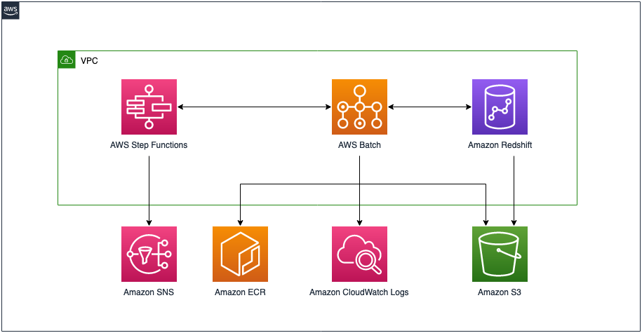
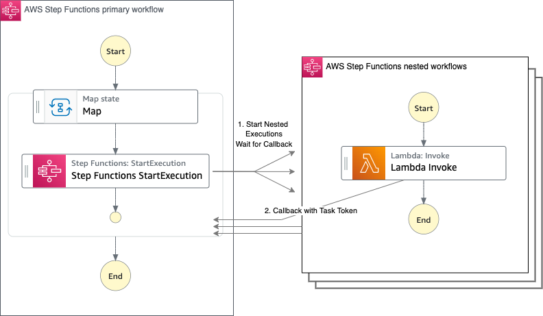
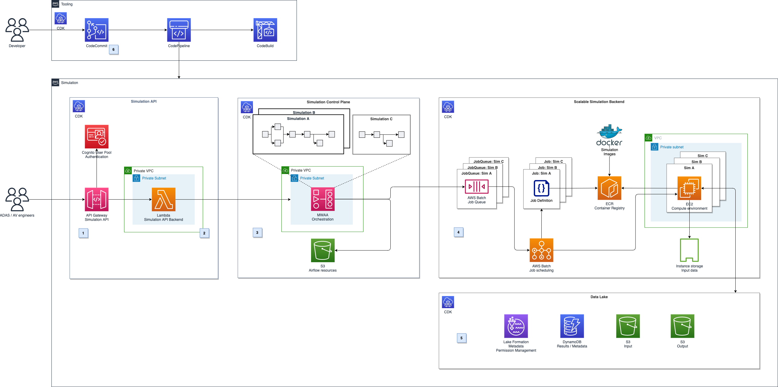
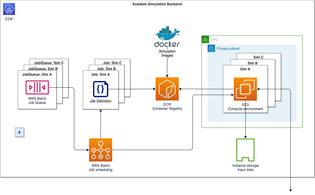
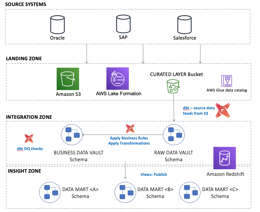
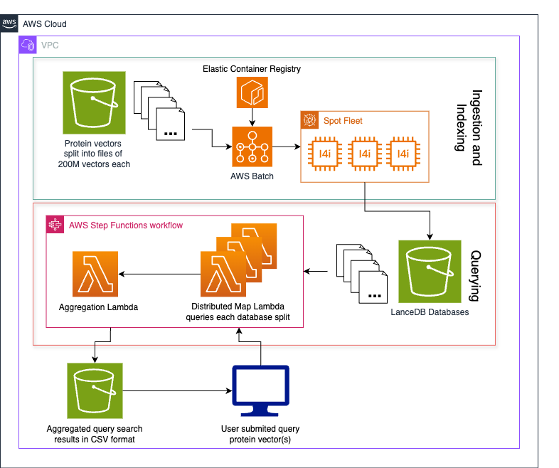
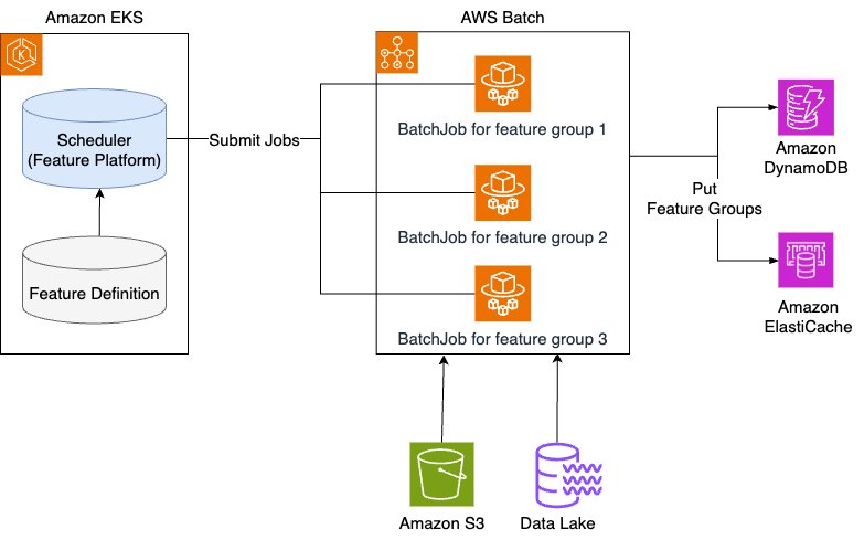
To overcome the challenge of ingesting and querying billions of vector embeddings representing Metagenomi’s large protein database, we devised a method for splitting the database into equal sized parts (folders) stored for low cost on Amazon S3 that can be indexed in parallel and searched with a map-reduce approach using Lambda. The following diagram illustrates this architecture.
The process follows four steps:
- Data vectorization
- Data bucketing
- Indexing and ingesting data
- Querying the database
Data vectorization
To make use of LanceDB’s fast ANN search capabilities, the data must be in vector form. Our metagenomics database consists of billions of proteins, each a string of amino acids. To convert each protein into a vector that captures biologically meaningful information, we run them through a protein language model (pLM), capturing the model’s hidden layers as a vector representation of that protein. Many pLMs can be used to generate protein embeddings, depending on the desired biological information and computational requirements. Here, we use the AMPLIFY_350M model, a transformer encoder model that is fast enough to scale to our entire protein database. We perform a mean-pool of the final hidden layer of the model to produce a 960-dimension vector for each protein. These vectors and their respective unique protein IDs are then stored in HDF5 files.
Data bucketing
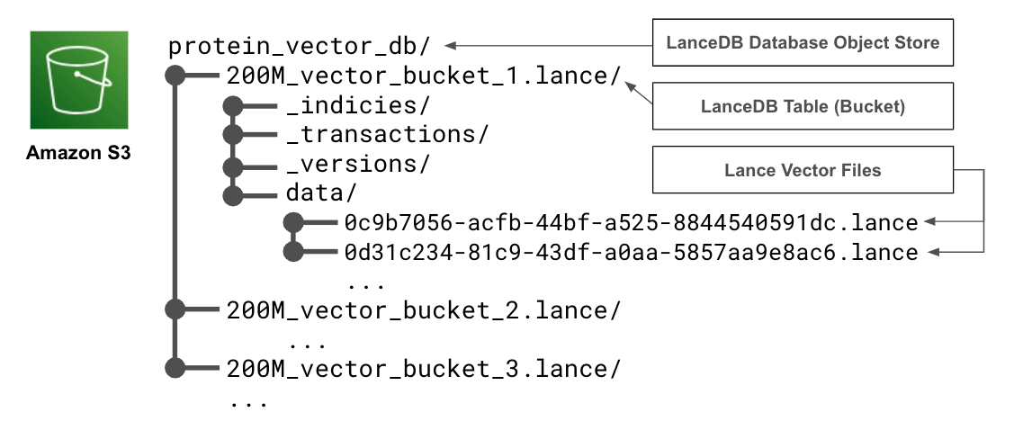
To turn our protein vectors into a searchable database, we use LanceDB to build an index suitable for quickly finding ANNs to a query. However, indexing can take a long time and is difficult to distribute across nodes. To speed up indexing, we first divide our data into roughly evenly sized buckets. We then assign each of our embedding HDF5 files to buckets of size roughly equal to 200 million total vectors using a best-fit bin packing algorithm. The exact size packing method used to bucket data depends on the number and dimension of the vectors, as well as their format. Each bucket is ingested into a separate table that will separately reside in a single LanceDB database object store on Amazon S3.
By bucketing our data, we can produce several smaller databases that can be indexed on separate nodes in a much shorter amount of time. We can also add more data to our database incrementally as a new bucket, instead of reindexing all the existing data.
Ingesting and indexing bucketed data
After the vectorized data has been assigned to a bucket, it’s time to turn it into a LanceDB table and index it to enable fast ANN querying. The details on how to convert your specific data into a LanceDB table can be found in the LanceDB documentation. For each of our buckets of approximately 200 million vectors, we create a LanceDB table with an IVF-PQ index on the cosine distance. For indexing, we use several partitions equal to the square root of the number of inserted rows, and several sub vectors equal to the number of dimensions of our vectors divided by 16.
To make things smoother to query, we name each table after the bucket from which it was created and upload them to a single S3 directory such that their file structure indicates a single LanceDB database with multiple tables.
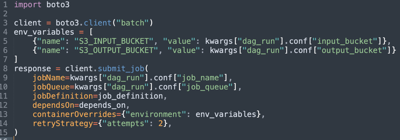
The following code snippet provides an example of how you might ingest vectors from an HDF5 file containing id and embedding columns into a LanceDB database and index for fast ANN searches based on cosine distance. The only requirements for running this snippet are python >= 3.9, as well as the lancedb, pyarrow, and h5py packages. It should be noted that this snippet was tested and developed using lancedb version 0.21.1 using the asynchronous LanceDB API.
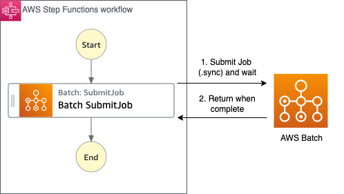
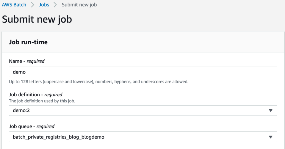
The task of vectorizing, ingesting, indexing each bucket could be parallelized over multiple AWS Batch jobs or run on a single Amazon Elastic Compute Cloud (Amazon EC2) instance.
Querying the database
After the data has been bucketed and ingested into a LanceDB database on Amazon S3, we need a way to query it. Because LanceDB can be queried directly from Amazon S3 using the LanceDB Python API, we can use Lambda functions to take a user-provided query vector and search for ANNs, then return the data to the user. However, because our data has been bucketed across several tables in the database, we need to search for nearest neighbors in each bucket and aggregate the results before passing them back to the user.
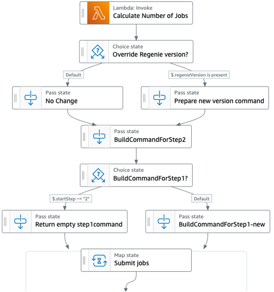
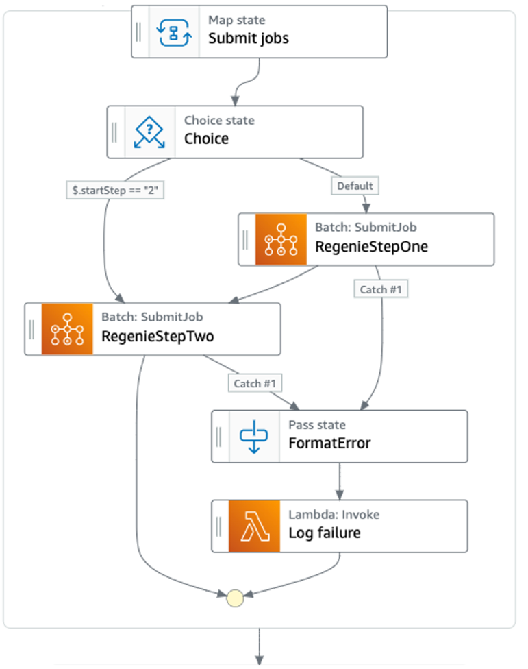
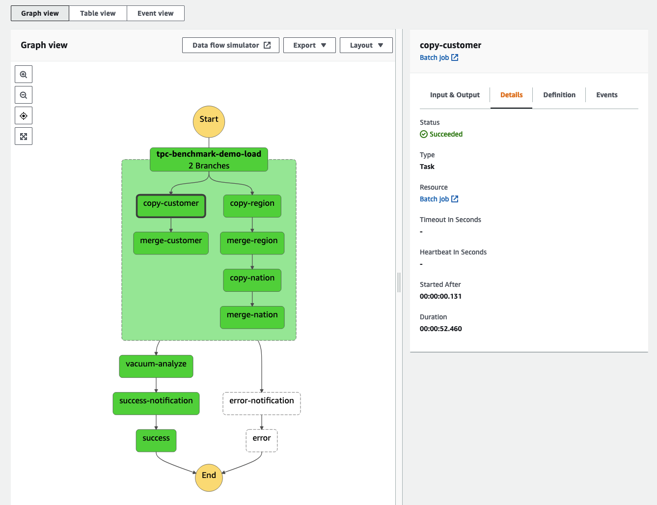
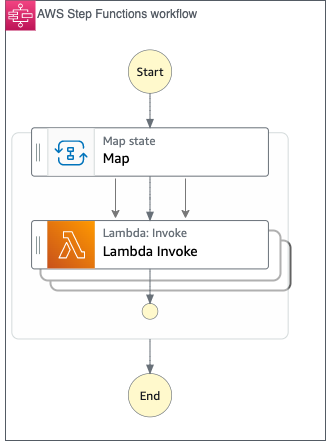
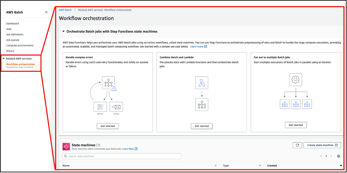
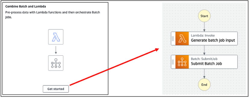
We implement the query workflow as an AWS Step Functions state machine that manages a query process for each bucket as Lambda processes, as well as a single Lambda process at the end that aggregates the data and writes the resulting ANNs to a .csv file on Amazon S3. However, this could also be implemented as a series of AWS Batch processes or even run locally. The following snippet shows how a process assigned to one bucket could run an ANN query against one of the database’s buckets, requiring only pandas and lancedb to run on python >= 3.9. As detailed before in the ingestion section, we use the asynchronous LanceDB API and lancedb package version 0.21.1.
The preceding query will return a panda DataFrame of the following structure:
| embedding | id | _distance |
| [-5.124435, 4.242000, …] | id_1 | 0.000000 |
| [-5.783999, 4.340500, …] | id_2 | 0.001000 |
| [-6.932943, 3.394850, …] | id_3 | 0.04020 |
Where the embedding column contains the vector representations of the nearest neighbors, the id column their IDs, and the _distance column their cosine distances to the queried vector.
After each bucket has been independently queried across nodes and each has returned a nearest neighbors DataFrame, the results must be merged and subset to return the user. The following snippet shows how you might do this.
Optimizing for large batches of queries
Though querying a LanceDB database directly from its S3 object store on Lambda works well for querying the ANNs of one or a few query vectors, some use cases might require querying thousands or even millions of vectors.
One solution we’ve found that scales well to large batches of queries is to modify the preceding query implementation such that it first downloads one of the database buckets to local storage, then queries it locally using the LanceDB API. Because database buckets can have a large storage footprint, this implementation is better suited for AWS Batch jobs than Lambda, and we recommend using optimized instance storage (for example, i4i instances) rather than EBS volumes. After all query Batch jobs finish, a final job can aggregate their results before returning to the user. Orchestration of parallel query jobs and the aggregation job can be done with Nextflow. Though this implementation will have significantly more overhead and latency from downloading the buckets to disk, it can handle larger batches of queries more efficiently and still requires no continuously running server-based database.
Benchmarking results
Indexing strategies and database split sizes depend on your personal need for performance. Consider the following general optimization guidance when customizing to your use case.
An example database created by Metagenomi consisted of 3.5 billion vector embeddings produced by AMPLIFY, of dimension 960. Ingesting and indexing these 3.5B vector embeddings in split sizes of 200M vectors on i4i.8xlarge instances took 108 total compute hours. Because this solution is serverless and can be queried directly from its S3 object store, the only fixed cost of this database is its storage footprint on Amazon S3 (for an indexed database of 3.5B vectors, this is approximately 12.9 TB). Lambda queries can be an exceptionally low-cost querying solution, with many queries costing fractions of a cent.
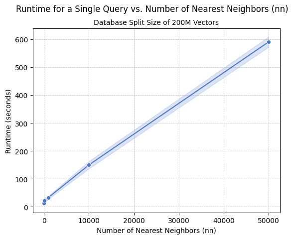
In general, larger database splits will be more cost effective to query but will result in longer runtimes and longer indexing times. We recommend scaling up database split sizes to the maximum size that results in an acceptable query return time for a single split while also considering limits of parallelization such as maximum concurrent Lambda functions running. Metagenomi identified database splits of 200M vectors each to yield an optimal trade-off in cost and runtime for both small and large queries. We recommend ingesting and indexing on storage-optimized instances, such as those in the i4i family, for optimal performance and cost savings. If querying is to be done on an instance using a disk-based database (as opposed to Lambda and Amazon S3), we also recommend using storage-optimized instances for queries. We found the Lambda implementation could quickly handle single queries requesting up to 50,000 ANNs, or multi queries of up to 100 sequences with fewer than 5 ANNs. Runtime increases linearly with the number of ANNs requested, as shown in the following graph.
Conclusion
In this post, we showed how Metagenomi was able to store and query billions of protein embeddings at low cost using LanceDB implemented with Amazon S3 and AWS Lambda. This work expands on Metagenomi’s patient-driven mission to create curative genetic medicines by accelerating our discovery and engineering platform. Having quick access to the ANN embedding space of a query protein in seconds has enabled the integration of rapid search methods in our extensive analysis pipelines, accelerated the discovery of several diverse and novel enzyme families, and enabled protein engineering efforts by providing scientists with methods to generate and search embeddings on the fly. As Metagenomi continues to rapidly scale protein and DNA databases, horizontal scaling enabled by database splits that can be indexed and searched in parallel facilitates an embedding database solution that scales to future needs.
The solution outlined in this post focuses on vectors produced by a protein large language model (LLM) but can be applied to other vectorized datasets. To learn more about LanceDB integrated with Amazon S3, refer to the LanceDB documentation.
References
- Fournier, Quentin, et al. “Protein language models: is scaling necessary?.” bioRxiv (2024): 2024-09.
 Jeff returns! This year, we have AWS “Chips” Taste Test for him to indulge in, drawing unique parallels between chip flavors and silicon innovations. He compared the taste of “Golden Nacho Cheese,” “Al Chili Lime,” and “BBQ Training Wheels” with