Post Syndicated from Yonatan Dolan original https://aws.amazon.com/blogs/big-data/melting-the-ice-how-natural-intelligence-simplified-a-data-lake-migration-to-apache-iceberg/

This post is co-written with Haya Axelrod Stern, Zion Rubin and Michal Urbanowicz from Natural Intelligence.

Many organizations turn to data lakes for the flexibility and scale needed to manage large volumes of structured and unstructured data. However, migrating an existing data lake to a new table format such as Apache Iceberg can bring significant technical and organizational challenges

Natural Intelligence (NI) is a world leader in multi-category marketplaces. NI’s leading brands, Top10.com and BestMoney.com, help millions of people worldwide to make informed decisions every day. Recently, NI embarked on a journey to transition their legacy data lake from Apache Hive to Apache Iceberg.

In this blog post, NI shares their journey, the innovative solutions developed, and the key takeaways that can guide other organizations considering a similar path.

This article details NI’s practical approach to this complex migration, focusing less on Apache Iceberg’s technical specifications, but rather on the real-world challenges and solutions encountered during the transition to Apache Iceberg, a challenge that many organizations are grappling with.

Why Apache Iceberg?

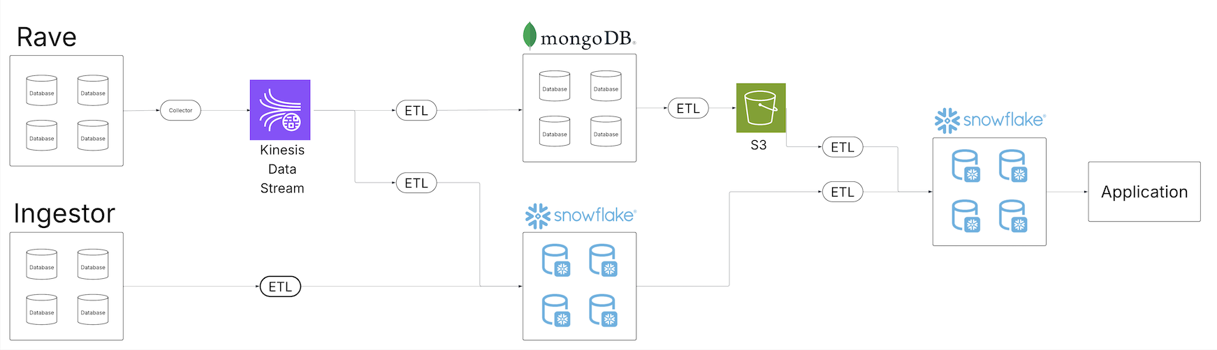
The architecture at NI followed the commonly used medallion architecture, comprised of a bronze-silver-gold layered framework, shown in the figure that follows:

• Bronze layer: Unprocessed data from various sources, stored in its raw format in Amazon Simple Storage Service (Amazon S3), ingested through Apache Kafka brokers.
• Silver layer: Contains cleaned and enriched data, processed using Apache Flink.
• Gold layer: Holds analytics-ready datasets designed for business intelligence (BI) and reporting, produced using Apache Spark pipelines, and consumed by services such as Snowflake, Amazon Athena, Tableau, and Apache Druid. The data is stored in Apache Parquet format with AWS Glue Catalog providing metadata management.

While this architecture supported NI analytical needs, it lacked the flexibility required for a truly open and adaptable data platform. The gold layer was coupled only with query engines that supported Hive and AWS Glue Data Catalog. It was possible to use Amazon Athena however Snowflake required maintaining another catalog in order to query those external tables. This issue made it difficult to evaluate or adopt alternative tools and engines without costly data duplication, query rewrite data catalog synchronization. As business scaled, NI needed a data platform that could seamlessly support multiple query engines simultaneously with a single data catalog and avoiding any vendor lock-in.

The power of Apache Iceberg

Apache Iceberg emerged as the perfect solution—a flexible, open table format that aligns with NI’s approach of Data Lake First. Iceberg offers several critical advantages such as ACID transactions, schema evolution, time travel, performance improvements and more. But the key strategic benefits lay in the ability to support multiple query engines simultaneously. It also has the following advantages:

• Decoupling of storage and compute: The open table format enables you to separate the storage layer from the query engine, allowing an easy swap and support for multiple engines concurrently without data duplication.
• Vendor independence: As an open table format, Apache Iceberg prevents vendor lock-in, giving you the flexibility to adapt to changing analytics needs.
• Vendor adoption: Apache Iceberg is widely supported by major platforms and tools, providing seamless integration and long-term ecosystem compatibility.

By transitioning to Iceberg, NI was able to embrace a truly open data platform, providing long-term flexibility, scalability, and interoperability while maintaining a unified source of truth for all analytics and reporting needs.

Challenges faced

Migrating a live production data lake to Iceberg was challenging because of operational complexities and legacy constraints. The data service at NI runs hundreds of Spark and machine learning pipelines, manages thousands of tables, and supports over 400 dashboards—all operating 24/7. Any migration would need to be done without production interruptions; and coordinating such a migration while operations continue seamlessly was daunting.

NI needed to accommodate diverse users with varying requirements and timelines from data engineers to data analysts all the way to data scientists and BI teams.

Adding to the challenge were legacy constraints. Some of the existing tools didn’t fully support Iceberg, so there was a need to maintain Hive-backed tables for compatibility. As NI realized that not all consumers could adopt Iceberg immediately. A plan was required to allow for incremental transitions without downtime or disruption to ongoing operations.

Key pillars for migration

To help ensure a smooth and successful transition, six critical pillars were defined:

• Support ongoing operations: Maintain uninterrupted compatibility with existing systems and workflows during the migration process.
• User transparency: Minimize disruption for users by preserving existing table names and access patterns.
• Gradual consumer migration: Allow consumers to adopt Iceberg at their own pace, avoiding a forced, simultaneous switchover.
• ETL flexibility: Migrate ETL pipelines to Iceberg without imposing constraints on development or deployment.
• Cost effectiveness: Minimize storage and compute duplication and overhead during the migration period.
• Minimize maintenance: Reduce the operational burden of managing dual table formats (Hive and Iceberg) during the transition.

Evaluating traditional migration approaches

Apache Iceberg supports two main approaches for migration: In-place and rewrite-based migration.

In-place migration

How it works: Converts an existing dataset into an Iceberg table without duplicating data by creating Iceberg metadata on top of the existing files while preserving their layout and format.

Advantages:

• Cost-effective in terms of storage (no data duplication)
• Simplified implementation
• Maintains existing table names and locations
• No data movement and minimal compute requirements, translating into lower cost

Disadvantages:

• Downtime required: All write operations must be paused during conversion, which was unacceptable in NI cases because data and analytics are considered mission critical and run 24/7
• No gradual adoption: All consumers must switch to Iceberg simultaneously, increasing the risk of disruption
• Limited validation: No opportunity to validate data before cutover; rollback requires restoring from backups
• Technical constraints: Schema evolution during migration can be challenging; data type incompatibilities can halt the entire process

Rewrite-based migration

How it works: Rewrite-based migration in Apache Iceberg involves creating a new Iceberg table by rewriting and reorganizing existing dataset files into Iceberg’s optimized format and structure for improved performance and data management.

Advantages:

• Zero downtime during migration
• Supports gradual consumer migration
• Enables thorough validation
• Simple rollback mechanism

Disadvantages:

• Resource overhead: Double storage and compute costs during migration
• Maintenance complexity: Managing two parallel data pipelines increases operational burden
• Consistency challenges: Maintaining perfect consistency between the two systems is challenging
• Performance impact: Increased latency because of dual writes; potential pipeline slowdowns

Why neither option alone was good enough

NI decided that neither option could meet all critical requirements:

• In-place migration fell short because of unacceptable downtime and lack of support for gradual migration.
• Rewrite-based migration fell short because of prohibitive cost overhead and complex operational management.

This analysis led NI to develop a hybrid approach that combines the advantages of both methods while mitigating and minimizing limitations.

The hybrid solution

The hybrid migration strategy was designed around five foundational elements, using AWS analytical services for orchestration, processing, and state management.

1. Hive-to-Iceberg CDC: Automatically synchronize Hive tables with Iceberg using a custom change data capture (CDC) process to support existing consumers. Unlike traditional CDC focusing on row-level changes, the process was done at the partition-level to preserve Hive’s behavior of updating tables by overwriting partitions. This helps ensure that data consistency is maintained between Hive and Iceberg without logic changes at the migration phase, making sure that the same data exists on both tables.
2. Continuous schema synchronization: Schema evolution during the migration introduced maintenance challenges. Automated schema sync processes compared Hive and Iceberg schemas, reconciling differences while maintaining type compatibility.
3. Iceberg-to-Hive reverse CDC: To enable the data team to transition extract, transform, and load (ETL) jobs to write directly to Iceberg while maintaining compatibility with existing Hive-based processes not yet migrated, a reverse CDC from Iceberg to Hive was implemented. This allowed ETLs to write to Iceberg while maintaining Hive tables for downstream processes that had not yet migrated and still relied on them during the migration period.
4. Alias management in Snowflake: Snowflake aliases made sure that Iceberg tables retained their original names, making the transition transparent to users. This approach minimized reconfiguration efforts across dependent teams and workflows.
5. Table replacement: Swap production tables while retaining original names, completing the migration.

Technical deep dive

The migration to from Hive to Iceberg was constructed of several steps:

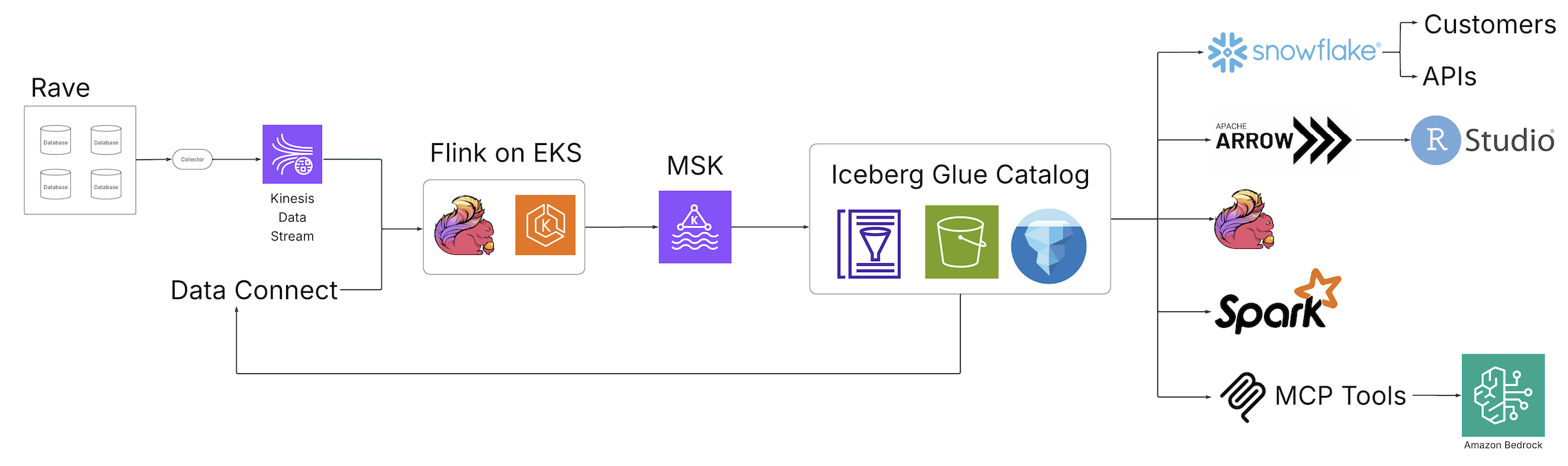
1. Hive-to-Iceberg CDC pipeline

Objective: Keep Hive and Iceberg tables synchronized without duplicating effort.

The preceding figure demonstrates how every partition written to the Hive table is automatically and transparently copied to the Iceberg table using a CDC process. This process makes sure that both tables are synchronized, enabling a seamless and incremental migration without disrupting downstream systems. NI chose partition-level synchronization because the legacy Hive ETL jobs already wrote updates by overwriting entire partitions and updating the partition location. Adopting that same approach in the CDC pipeline helped ensure that it remained consistent with how data was originally managed, making the migration smoother and avoiding the need to rework row-level logic.

Implementation:

• To keep Hive and Iceberg tables synchronized without duplicating effort, a streamlined pipeline was implemented. Whenever partitions in Hive tables are updated, the AWS Glue Catalog emits events such as UpdatePartition. Amazon EventBridge captured these events, filtered them for the relevant databases and tables according to the event bridge rule, and triggered an AWS Lambda This function parsed the event metadata and sent the partition updates to an Apache Kafka topic.
• A Spark job running on Amazon EMR consumed the messages from Kafka, which contained the updated partition details from the Data Catalog events. Using that event metadata, the Spark job queried the relevant Hive table, and wrote it to Iceberg table in Amazon S3 using the Spark Iceberg overwritePartitions API, as shown in the following example:

{
   "id":"10397e54-c049-fc7b-76c8-59e148c7cbfc",
   "detail-type":"Glue Data Catalog Table State Change",
   "source":"aws.glue",
   "time":"2024-10-27T17:16:21Z",
   "region":"us-east-1",
   "detail":{
      "databaseName":"dlk_visitor_funnel_dwh_production",
      "changedPartitions":[
         "2024-10-27"
      ],
      "typeOfChange":"UpdatePartition",
      "tableName":"fact_events"
   }
}

• By targeting only modified partitions, the pipeline (shown in the following figure) significantly reduced the need for costly full-table rewrites. Iceberg’s robust metadata layers, including snapshots and manifest files, were seamlessly updated to capture these changes, providing efficient and accurate synchronization between Hive and Iceberg tables.

2. Iceberg-to-Hive reverse CDC pipeline

Objective: Support Hive consumers while allowing ETL pipelines to transition to Iceberg.

The preceding figure shows the reverse process, where every partition written to the Iceberg table is automatically and transparently copied to the Hive table using a CDC mechanism. This process helps ensure synchronization between the two systems, enabling seamless data updates for legacy systems that still rely on Hive while transitioning to Iceberg.

Implementation:

Synchronizing data from Iceberg tables back to Hive tables presented a different challenge. Unlike Hive tables, Data Catalog doesn’t track partition updates for Iceberg tables because partitions in Iceberg are managed internally and not within the catalog. This meant NI couldn’t rely on Glue Catalog events to detect partition changes.

To address this, NI implemented a solution similar to the previous flow but adapted to Iceberg’s architecture. Apache Spark was used to query Iceberg’s metadata tables—specifically the snapshots and entries tables—to identify the partitions modified since the last synchronization. The query used was:

SELECT e.data_file.partition, MAX(s.committed_at) AS last_modified_time 
FROM $target_table.snapshots JOIN $target_table.entries e ON s.snapshot_id = e.snapshot_id 
WHERE s.committed_at > '$last_sync_time' 
GROUP BY e.data_file.partition;

This query returned only the partitions that had been updated since the last synchronization, enabling it to focus exclusively on the changed data. Using this information, similar to the earlier process, a Spark job retrieved the updated partitions from Iceberg and wrote them back to the corresponding Hive table, providing seamless synchronization between both tables.

3. Continuous schema synchronization

Objective: Automate schema updates to maintain consistency across Hive and Iceberg.

The preceding figure shows how the automatic schema sync process helps ensure consistency between Hive and Iceberg tables schemas by automatically synchronizing schema changes. In this example adding the Channel column, minimizing manual work and double maintenance during the extended migration period.

 Implementation:

To handle schema changes between Hive and Iceberg, a process was implemented to detect and reconcile differences automatically. When a schema change happens in a Hive table, Data Catalog emits an UpdateTable event. This event triggers a Lambda function (routed through EventBridge), which retrieves the updated schema from Data Catalog for the Hive table and compares it to the Iceberg schema. It’s important to call out that in NI’s setup, schema changes originate from Hive because the Iceberg table is hidden behind aliases across the system. Because Iceberg is primarily used for Snowflake, a one-way sync from Hive to Iceberg is sufficient. As a result, there is no mechanism to detect or handle schema changes made directly in Iceberg, because they aren’t needed in the current workflow.

During the schema reconciliation (shown in the following figure), data types are normalized to help ensure compatibility—for example, converting Hive’s VARCHAR to Iceberg’s STRING. Any new fields or type changes are validated and applied to the Iceberg schema using a Spark job running on Amazon EMR. Amazon DynamoDB stores schema synchronization checkpoints which allow tracking changes over time and maintain consistency between the Hive and Iceberg schemas.

By automating this schema synchronization, maintenance overhead was significantly reduced and freed developers from manually keeping schemas in sync, making the long migration period significantly more manageable.

The preceding figure depicts an automated workflow to maintain schema consistency between Hive and Iceberg tables. AWS Glue captures table state change events from Hive, which trigger an EventBridge event. The event invokes a Lambda function that fetches metadata from DynamoDB and compares schemas fetched from AWS Glue for both Hive and Iceberg tables. If a mismatch is detected, the schema in Iceberg is updated to help ensure alignment, minimizing manual intervention and supporting smooth operation during the migration.

4. Alias management in Snowflake

Objective: Enable Snowflake consumers to adopt Iceberg without changing query references.

The preceding figure shows how Snowflake aliases enable seamless migration by mapping queries like SELECT platform, COUNT(clickouts) FROM funnel.clickouts to Iceberg tables in the Glue Catalog. Even with suffixes added during the Iceberg migration, existing queries and workflows remain unchanged, minimizing disruption for BI tools and analysts.

Implementation:

To help ensure a seamless experience for BI tools and analysts during the migration, Snowflake aliases were used to map external tables to the Iceberg metadata stored in Data Catalog. By assigning aliases that matched the original Hive table names, existing queries and reports were preserved without interruption. For example, an external table was created in Snowflake and aliased it to the original table name, as shown in the following query:

CREATE OR REPLACE ICEBERG TABLE dlk_visitor_funnel_dwh_production.aggregated_cost 
EXTERNAL_VOLUME = 's3_dlk_visitor_funnel_dwh_production_iceberg_migration' 
CATALOG = 'glue_dlk_visitor_funnel_dwh_production_iceberg_migration' 
CATALOG_TABLE_NAME = 'aggregated_cost'; 
ALTER ICEBERG TABLE dlk_visitor_funnel_dwh_production.aggregated_cost REFRESH;

When migration was completed, a simple change back to the alias was done to point to the new location or schema, making the transition seamless and minimizing any disruption to user workflows.

5. Table replacement

Objective: When all ETLs and related data workflows were successfully transitioned to use Apache Iceberg’s capabilities, and everything was functioning correctly with the synchronization flow, it was time to move on to the final phase of the migration. The primary objective was to maintain the original table names, avoiding the use of any prefixes like those employed in the earlier, intermediate migration steps. This helped ensure that the configuration remained tidy and free from unnecessary naming complications.

The preceding figure shows the table replacement to complete the migration, where Hive on Amazon EMR was used to register Parquet files as Iceberg tables while preserving original table names and avoiding data duplication, helping to ensure a seamless and tidy migration.

Implementation:

One of the challenges was that renaming tables isn’t possible within AWS Glue, which prevents the use of a straightforward renaming approach for the existing synchronization flow tables. In addition, AWS Glue doesn’t support the Migrate procedure, which creates Iceberg metadata on top of the existing data file while preserving the original table name. The strategy to overcome this limitation was to use a Hive metastore on an Amazon EMR cluster. By using Hive on Amazon EMR, NI was able to create the final tables with their original names because it operates in a separate metastore environment, giving the flexibility to define any required schema and table names without interference.

The add_files procedure was used to methodically register all the existing Parquet files, thus constructing all necessary metadata within Hive. This was a crucial step, because it helped ensure that all data files were appropriately cataloged and linked within the metastore.

The preceding figure shows the transition of a production table to Iceberg by using the add_files procedure to register existing Parquet files and create Iceberg metadata. This helped ensure a smooth migration while preserving the original data and avoiding duplication.

This setup allowed the use of existing Parquet files without duplicating data, thus saving resources. Although the sync flow used separate buckets for the final architecture, NI chose to maintain the original buckets and cleaned the intermediate files. This resulted in a different folder structure on Amazon S3. The historical data had subfolders for each partition under the root table directory, while the new Iceberg data organizes subfolders within a data folder. This difference was acceptable to avoid data duplication and preserve the original Amazon S3 buckets.

Technical recap

The AWS Glue Data Catalog served as the primary source of truth for schema and table updates, with Amazon EventBridge capturing Data Catalog events to trigger synchronization workflows. AWS Lambda parsed event metadata and managed schema synchronization, while Apache Kafka buffered events for real-time processing. Apache Spark on Amazon EMR handled data transformations and incremental updates, and Amazon DynamoDB maintained state, including synchronization checkpoints and table mappings. Finally, Snowflake seamlessly consumed Iceberg tables via aliases without disrupting existing workflows.

Migration outcome

The migration was completed with zero downtime; continuous operations were maintained throughout the migration, supporting hundreds of pipelines and dashboards without interruption. The migration was done with a cost optimized mindset with incremental updates and partition-level synchronization that minimized the usage of compute and storage resources. Lastly, NI Established a modern, vendor-neutral platform that enables scaling their evolving analytics and machine learning needs. It enables seamless integration with multiple compute and query engines, supporting flexibility and further innovation.

Conclusion

Natural intelligence migration to Apache Iceberg was a pivotal step in modernizing the company’s data infrastructure. By adopting a hybrid strategy and using the power of event-driven architectures, NI helped ensure a seamless transition that balanced innovation with operational stability. The journey underscored the importance of careful planning, understanding the data ecosystem, and focusing on an organization-first approach.

Above all, business was kept in focus and continuity prioritized the user experience. By doing so, NI unlocked the flexibility and scalability of their data lake while minimizing disruption, allowing teams to use cutting-edge analytics capabilities, positioning the company at the forefront of modern data management and readiness for the future.

If you’re considering an Apache Iceberg migration or facing similar data infrastructure challenges, we encourage you to explore the possibilities. Embrace open formats, use automation, and design with your organization’s unique needs in mind. The journey might be complex, but the rewards in scalability, flexibility, and innovation are well worth the effort. You can use the AWS prescriptive guide to help learn more about how to best use Apache Iceberg for your organization

About the Authors

Yonatan Dolan is a Principal Analytics Specialist at Amazon Web Services. Yonatan is an Apache Iceberg evangelist.

Haya Stern is a Senior Director of Data at Natural Intelligence. She leads the development of NI’s large-scale data platform, with a focus on enabling analytics, streamlining data workflows, and improving dev efficiency. In the past year, she led the successful migration from the previous data architecture to a modern lake house based on Apache Iceberg and Snowflake.

Zion Rubin is a Data Architect at Natural Intelligence with ten years of experience architecting large‑scale big‑data platforms, now focused on developing intelligent agent systems that turn complex data into real‑time business insight.

Michał Urbanowicz is a Cloud Data Engineer at Natural Intelligence with expertise in migrating data warehouses and implementing robust retention, cleanup, and monitoring processes to ensure scalability and reliability. He also develops automations that streamline and support campaign management operations in cloud-based environments.