Post Syndicated from Dylan Qu original https://aws.amazon.com/blogs/big-data/simplify-your-etl-and-ml-pipelines-using-the-amazon-athena-unload-feature/
Many organizations prefer SQL for data preparation because they already have developers for extract, transform, and load (ETL) jobs and analysts preparing data for machine learning (ML) who understand and write SQL queries. Amazon Athena is an interactive query service that makes it easy to analyze data in Amazon Simple Storage Service (Amazon S3) using standard SQL. Athena is serverless, so there is no infrastructure to manage, and you pay only for the queries that you run.
By default, Athena automatically writes SELECT query results in CSV format to Amazon S3. However, you might often have to write SELECT query results in non-CSV files such as JSON, Parquet, and ORC for various use cases. In this post, we walk you through the UNLOAD statement in Athena and how it helps you implement several use cases, along with code snippets that you can use.
Athena UNLOAD overview
CSV is the only output format used by the Athena SELECT query, but you can use UNLOAD to write the output of a SELECT query to the formats and compression that UNLOAD supports. When you use UNLOAD in a SELECT query statement, it writes the results into Amazon S3 in specified data formats of Apache Parquet, ORC, Apache Avro, TEXTFILE, and JSON.
Although you can use the CTAS statement to output data in formats other than CSV, those statements also require the creation of a table in Athena. The UNLOAD statement is useful when you want to output the results of a SELECT query in a non-CSV format but don’t require the associated table. For example, a downstream application might require the results of a SELECT query to be in JSON format, and Parquet or ORC might provide a performance advantage over CSV if you intend to use the results of the SELECT query for additional analysis.
In this post, we walk you through the following use cases for the UNLOAD feature:
- Compress Athena query results to reduce storage costs and speed up performance for downstream consumers
- Store query results in JSON file format for specific downstream consumers
- Feed downstream Amazon SageMaker ML models that require files as input
- Simplify ETL pipelines with AWS Step Functions without creating a table
Use case 1: Compress Athena query results
When you’re using Athena to process and create large volumes of data, storage costs can increase significantly if you don’t compress the data. Furthermore, uncompressed formats like CSV and JSON require you to store and transfer a large number of files across the network, which can increase IOPS and network costs. To reduce costs and improve downstream big data processing application performance such as Spark applications, a best practice is to store Athena output into compressed columnar compressed file formats such as ORC and Parquet.
You can use the UNLOAD statement in your Athena SQL statement to create compressed ORC and Parquet file formats. In this example, we use a 3 TB TPC-DS dataset to find all items returned between a store and a website. The following query joins the four tables: item, store_returns, web_returns, and customer_address:
The resulting query output when Snappy compressed and stored in Parquet format resulted in a 62 GB dataset. The same output in a non-compressed CSV format resulted in a 248 GB dataset. The Snappy compressed Parquet format yielded a 75% smaller storage size, thereby saving storage costs and resulting in faster performance.
Use case 2: Store query results in JSON file format
Some downstream systems to Athena such as web applications or third-party systems require the data formats to be in JSON format. The JSON file format is a text-based, self-describing representation of structured data that is based on key-value pairs. It’s lightweight, and is widely used as a data transfer mechanism by different services, tools, and technologies. In these use cases, the UNLOAD statement with the parameter format value of JSON can unload files in JSON file format to Amazon S3.
The following SQL extracts the returns data for a specific customer within a specific data range against the 3 TB catalog_returns table and stores it to Amazon S3 in JSON format:
By default, Athena uses Gzip for JSON and TEXTFILE formats. You can set the compression to NONE to store the UNLOAD result without any compression. The query result is stored as the following JSON file:
The query result can now be consumed by a downstream web application.
Use case 3: Feed downstream ML models
Analysts and data scientists rely on Athena for ad hoc SQL queries, data discovery, and analysis. They often like to quickly create derived columns such as aggregates or other features. These need to be written as files in Amazon S3 so a downstream ML model can directly read the files without having to rely on a table.
You can also parametrize queries using Athena prepared statements that are repetitive. Using the UNLOAD statement in a prepared statement provides the self-service capability to less technical users or analysts and data scientists to export files needed for their downstream analysis without having to write queries.
In the following example, we create derived columns and feature engineer for a downstream SageMaker ML model that predicts the best discount for catalog items in future promotions. We derive averages for quantity, list price, discount, and sales price for promotional items sold in stores where the promotion is not offered by mail or a special event. Then we restrict the results to a specific gender, marital, and educational status. We use the following query:
The output is written as Parquet files in Amazon S3 for a downstream SageMaker model training job to consume.
Use case 4: Simplify ETL pipelines with Step Functions
Step Functions is integrated with the Athena console to facilitate building workflows that include Athena queries and data processing operations. This helps you create repeatable and scalable data processing pipelines as part of a larger business application and visualize the workflows on the Athena console.
In this use case, we provide an example query result in Parquet format for downstream consumption. In this example, the raw data is in TSV format and gets ingested on a daily basis. We use the Athena UNLOAD statement to convert the data into Parquet format. After that, we send the location of the Parquet file as an Amazon Simple Notification Service (Amazon SNS) notification. Downstream applications can be notified via SNS to take further actions. One common example is to initiate a Lambda function that uploads the Athena transformation result into Amazon Redshift.
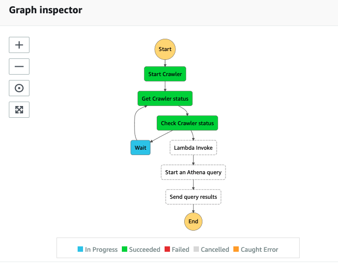
The following diagram illustrates the ETL workflow.

The workflow includes the following steps:
- Start an AWS Glue crawler pointing to the raw S3 bucket. The crawler updates the metadata of the raw table with new files and partitions.
- Invoke a Lambda function to clean up the previous UNLOAD result. This step is required because UNLOAD doesn’t write data to the specified location if the location already has data in it (UNLOAD doesn’t overwrite existing data). To reuse a bucket location as a destination for UNLOAD, delete the data in the bucket location, and then run the query again. Another common pattern is to UNLOAD data to a new partition with incremental data processing.
- Start an Athena UNLOAD query to convert the raw data into Parquet.
- Send a notification to downstream data consumers when the file is updated.
Set up resources with AWS CloudFormation
To prepare for querying both data sources, launch the provided AWS CloudFormation template:
![]()
Keep all the provided parameters and choose Create stack.
The CloudFormation template creates the following resources:
- An Athena workgroup
etl-workgroup, which holds the Athena UNLOAD queries. - A data lake S3 bucket that holds the raw table. We use the Amazon Customer Reviews Dataset in this post.
- An Athena output S3 bucket that holds the UNLOAD result and query metadata.
- An AWS Glue database.
- An AWS Glue crawler pointing to the data lake S3 bucket.
- A
LoadDataBucketLambda function to load the Amazon Customer Reviews raw data into the S3 bucket. - A
CleanUpS3FolderLambda function to clean up previous Athena UNLOAD result. - An SNS topic to notify downstream systems when the UNLOAD is complete.
When the stack is fully deployed, navigate to the Outputs tab of the stack on the AWS CloudFormation console and note the value of the following resources:
AthenaWorkgroupAthenaOutputBucketCleanUpS3FolderLambdaGlueCrawlerSNSTopic
Build a Step Functions workflow
We use the Athena Workflows feature to build the ETL pipeline.
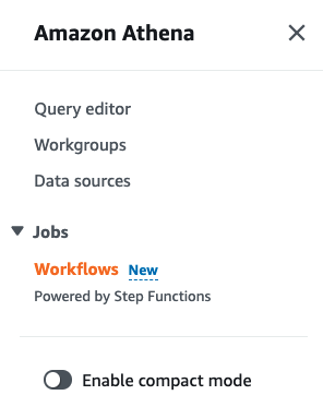
- On the Athena console, under Jobs in the navigation pane, choose Workflows.

- Under Create Athena jobs with Step Functions workflows, for Query large datasets, choose Get started.
- Choose Create your own workflow.
- Choose Continue.
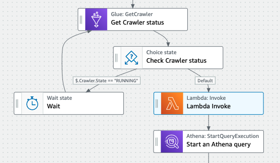
The following is a screenshot of the default workflow. Compare the default workflow against the earlier ETL workflow we described. The default workflow doesn’t contain a Lambda function invocation and has an additional GetQueryResult step.

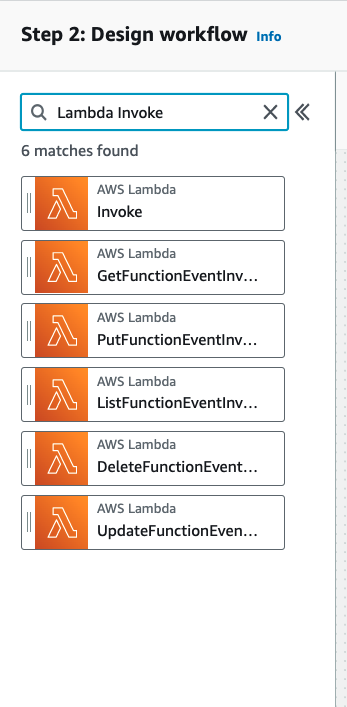
Next, we add a Lambda Invoke step.
- Search for
Lambda Invokein the search bar.

- Choose the Lambda:Invoke step and drag it to above the Athena: StartQueryExecution step.

- Choose the Athena:GetQueryResults step (right-click) and choose Delete state.

- Now the workflow aligns with the earlier design.

- Choose the step Glue: StartCrawler.
- In the Configuration section, under API Parameters, enter the following JSON (provide the AWS Glue crawler name from the CloudFormation stack output):
- Choose the step Glue: GetCrawler.
- In the Configuration section, under API Parameters, enter the following JSON:
- Choose the step Lambda: Invoke.
- In the Configuration section, under API Parameters, for Function name, choose the function
-CleanUpS3FolderLambda-. - In the Payload section, enter the following JSON (include the Athena output bucket from the stack output):
- Choose the step Athena: StartQueryExecution.
- In the right Configuration section, under API Parameters, enter the following JSON (provide the Athena output bucket and workgroup name):


Notice the Wait for task to complete check box is selected. This pauses the workflow while the Athena query is running.
- Choose the step SNS: Publish.
- In the Configuration section, under API Parameters, for Topic, pick the
SNSTopiccreated by the CloudFormation template. - In the Message section, enter the following JSON to pass the data manifest file location to the downstream consumer:
For more information, refer to the GetQueryExecution response syntax.
- Choose Next.
- Review the generated code and choose Next.
- In the Permissions section, choose Create new role.
- Review the auto-generated permissions and choose Create state machine.
- In the Add additional permissions to your new execution role section, choose Edit role in IAM.

- Add permissions and choose Attach policies.

- Search for the
AWSGlueConsoleFullAccessmanaged policy and attach it.


This policy grants full access to AWS Glue resources when using the AWS Management console. Generate a policy based on access activity in production following the least privilege principle.
Test the workflow
Next, we test out the Step Functions workflow.
- On the Athena console, under Jobs in the navigation pane, choose Workflows.
- Under State machines, choose the workflow we just created.
- Choose Execute, then choose Start execution to start the workflow.

- Wait until the workflow completes, then verify there are UNLOAD Parquet files in the bucket
AthenaOutputBucket.


Clean up
To help prevent unwanted charges to your AWS account, delete the AWS resources that you used in this post.
- On the Amazon S3 console, choose the
-athena-unload-data-lakebucket. - Select all files and folders and choose Delete.
- Enter
permanently deleteas directed and choose Delete objects. - Repeat these steps to remove all files and folders in the
-athena-unload-outputbucket. - On the AWS CloudFormation console, delete the stack you created.
- Wait for the stack status to change to
DELETE_COMPLETE.
Conclusion
In this post, we introduced the UNLOAD statement in Athena with some common use cases. We demonstrated how to compress Athena query results to reduce storage costs and improve performance, store query results in JSON file format, feed downstream ML models, and create and visualize ETL pipelines with Step Functions without creating a table.
To learn more, refer to the Athena UNLOAD documentation and Visualizing AWS Step Functions workflows from the Amazon Athena console.
About the Authors
 Dylan Qu is a Specialist Solutions Architect focused on Big Data & Analytics with Amazon Web Services. He helps customers architect and build highly scalable, performant, and secure cloud-based solutions on AWS.
 Harsha Tadiparthi is a Principal Solutions Architect focused on providing analytics and AI/ML strategies and solution designs to customers.


 Dylan Qu is an AWS solutions architect responsible for providing architectural guidance across the full AWS stack with a focus on Data Analytics, AI/ML and DevOps.
 Vishwa Gupta is a Data and ML Engineer with AWS Professional Services Intelligence Practice. He helps customers implement big data and analytics solutions. Outside of work, he enjoys spending time with family, traveling, and playing badminton.


 Rob Craig is a Senior Solutions Architect with AWS. He supports customers in the UK with their cloud journey, providing them with architectural advice and guidance to help them achieve their business outcomes.
 Dylan Qu is an AWS solutions architect responsible for providing architectural guidance across the full AWS stack with a focus on Data Analytics, AI/ML and DevOps.